
1
Traditional Valuation Methods and Ways of Applying Them
1.1. Introduction
It is imperative that the investments of a business generate a sufficient level of profitability to satisfy the demands held by the investors. If the obtained (or predicted) level of profitability is higher than the level of profitability that is expected given the risk, the value of the economic asset increases, impacting the value of shares in an upward fashion1. Otherwise, the investor will not be satisfied with the profitability of their investment in relation to the risk absorbed to sell their security. Enterprise and share value thus will fluctuate in a downwards fashion. And so, the direct consequence of the investment policy is a variation in economic value of equity, i.e. the market capitalization if the company is listed2. It thus follows that an investor’s power lies, on the one hand, in their decision to allocate funds to the company (without financial backing, the company is no more) and, on the other hand, in the evaluation of the economic asset through securities that have already been issued3. Consequently, changes in the value of economic assets are reflected almost entirely on market capitalization. When the company faces significant difficulties, the role of creditors changes because from a financial perspective, they then own the company. When the equity value is almost zero, adjustments can only be made through the net debt, whose value becomes lower than the nominal value. Therefore, liabilities are the screen placed between the value of economic assets and the financial decisions taken by investors.
Just as the investment policy is able to create or destroy value, the financial policy through the financial structure can theoretically change the value of equity. It is not so much of question of increasing the free cash flow of economic assets as it is of reducing the weighted average cost of capital, synonymous with the financial cost of the company, i.e. the minimum rate of return that assets must generate. In this way, it seems pertinent to interrogate whether an optimal liability structure can be created. The said structure would enable the cost of capital to be minimized, thereby maximizing the enterprise value.
To guide their decisions to allocate their resources to companies, investors use traditional valuation methods. In this way, the economic valuation of shareholder equity can be obtained by relying on a stock market analysis by comparing the aggregate multiples of the balance sheet and/or the income statement, or by undertaking a transactional comparison of the processes being carried out in the sector that the company to be valued operates in. Furthermore, by producing a business plan, i.e. by providing free cash flows that are discounted at the cost of capital, the investors may estimate the value of the company based on its future plans. Finally, by adopting a proprietary approach, investors are able to concentrate on the real assets held at a given time by the company. These three approaches are in theory supposed to be combined in order to refine the valuation further. With this in mind, it becomes ever more important to investigate whether an optimal capital structure really exists. Indeed, when it comes to carrying out a valuation by discounting free cash flows, two possibilities arise in terms of maximizing the enterprise value. Either the investment policy is relevant in itself, as it generates significant cash flows which lie in the numerator of the formula, or it is possible to consider that an adequate financial policy is carried out on condition that it decreases the cost of capital, which is at the denominator of the formula. In both of these scenarios, the enterprise value is increased.
Auditing activities come in particular from this type of valuation exercise. Theories from organizations, which help to explain the levels of corporate debts, go beyond outlining how to adopt acquisition strategies. Indeed, the very nature of shareholding encourages one to implement different types of financial arrangement that influence both the evolution of the power of holders of capital and the choice of which financial structure to adopt in order to acquire the target company.
1.2. The cost of financial structure
The portfolio theory from Markovitz (1959) deals with determining the cost of equity. The investor’s profitability demand depends on their degree of risk aversion. The portfolio to be chosen is graphically located at the intersection of the efficient frontier and one of the curves that characterizes the investor’s iso-utility. Sharpe (1963) simplifies this theory by assuming that the expected return on an asset is linked to the return on a market index. Thus, the investor’s demand for profitability depends solely on systematic risk. Efficient diversification of an asset portfolio eliminates the specific risk of the share.
An economic reading of a balance sheet consists of identifying, at a given moment, all the jobs involved in the company’s operating cycle and the origin of its resources. Economic assets (or enterprise value) are the sum of fixed assets and working capital requirements, i.e. all of the network in progress that is aligned with the operating and investment cycle4. Economic assets are financed by equity and net debt. And so, the market value of the economic asset is divided between the market value of these two types of resources. This results in a balance sheet of the company that only includes market values. In this context, the question arises as to whether there is an optimal capital structure that maximizes enterprise value and thereby minimizes the cost of capital.
The traditional approach, wherein evaluation is carried out without taxation, ensures that there is an optimal liability structure resulting from a sound use of the leverage effect. By also considering a tax-free approach, equilibrium market theory asserts, on the contrary, that there is no optimal capital structure because investors are able to duplicate at their level the financial operations of companies without cost and without any additional risk. The arbitrations that they can mobilize in the event of initial situations where the financial structures would be different lead to a rebalancing of the market. That is to say, they help to ensure that the value of the financial liabilities of two companies that are equal in every aspect becomes equal again. In the presence of taxation, the value of an indebted company is equal to that of a company that is not indebted, to which we must add to the present value of the tax savings linked to the tax deductibility of interest charges. However, even in the presence of taxation, the theories presented by organizations teach us that the choice of whether or not to go into debt comes more from the agent conflicts between the different parties such as shareholders and creditors, or from signals sent to the market more than from intrinsic costs.
1.2.1. Financial asset valuation
The models for valuating financial assets or the capital assets pricing model (CAPM) is used to evaluate the equity of a company in a balanced market. This formula provides an estimate of the rate of return expected by the market for a financial asset according to its systematic risk.
Markowitz (1959) states that between two portfolios characterized by their supposedly random return, one would retain, at identical risk, the company with the highest expected return and, with the same expected return, the company with the lower risk. This principle means that a number of portfolios may be dismissed, as they are less efficient than others. The efficient frontier represents the curve that connects the set of efficient portfolios. The portfolios that sit below this curve are rejected.
Consequently, it is possible to determine the weight of two assets that appear in a portfolio in order to minimize the risk thereof:
or:
- – Rp: portfolio return;
- – xi: weight of asset i in the portfolio.
Variance is minimal when its derivative is zero. We then look for xA such that:
As a result:
Now considering Rp, the portfolio return made up of n assets characterized by their respective return R1..., Rn, we have:
In order to determine E(Rp) and V(Rp), we suppose that:
Assume first that the returns of each of the n assets fluctuate independently of each other. In this case, the variance of a sum is equal to the sum of its variances. And so:
If n approaches infinity, then ![]() goes to 0.
goes to 0.
We then suppose that the performance of each of the n assets is correlated with each other. In this case:
where:
Let ![]() be the average covariance of portfolio P. By definition:
be the average covariance of portfolio P. By definition:
where N corresponds to the number of covariances.
In total, the number N of terms is equal to 0 + 1 + ... + (n – 1), so:
Like:
One has:
Consequently:
When n approaches infinity, ![]() approaches 0 and
approaches 0 and ![]() approaches the ratio of terms of higher degree. This ratio is equal to 1. By multiplying this result by
approaches the ratio of terms of higher degree. This ratio is equal to 1. By multiplying this result by ![]() , we may deduce that V(Rp) approaches the mean covariance
, we may deduce that V(Rp) approaches the mean covariance ![]() The risk equal to the standard deviation of Rp cannot therefore be eliminated, even by diversifying the portfolio insofar as it therefore approaches the square root of the mean covariance.
The risk equal to the standard deviation of Rp cannot therefore be eliminated, even by diversifying the portfolio insofar as it therefore approaches the square root of the mean covariance.
On the graph, this means that the curve that represents the risk as a function of the number of securities that are contained within the portfolio admits a horizontal asymptote of equation ![]() .
.
The basis of the CAPM comes from the hypothesis within the Markowitz model, i.e. a portfolio for which performance Rp is defined as:
We assume moreover that the performance Ri of each asset i is linearly related to a market index denoted I. In other words, ![]() , where I and
, where I and ![]() are a random variable that presents the following properties:
are a random variable that presents the following properties:
- –

- –
 constant;
 - –
 for 2 assets i and j becoming part of the portfolio.
In this case, the choice of portfolio located on the efficient frontier which should be retained according to the degree of the investor’s risk aversion is simpler. It comes from solving a system of equations that correspond to the inversion of an almost diagonal matrix (it is then necessary to consider the inverses of the numbers located on the diagonal). The financial asset equilibrium model, from which the formula for the capital market line (used to determine the cost of equity) is derived, makes the simplified hypothesis model from Sharpe (1963) endogenous. In other words, this method consists of replacing the index I from the Sharpe formula with the performance RM of the whole market.
The formula is thus:
When looking at a portfolio P composed of n assets i each of them entering for a proportion Xi, the portfolio yield is as follows:
We can thus calculate:
And then:
As a result, the beta of a portfolio is the weighted average of the betas of the assets that make it up.
Let us consider a portfolio composed of a market index contract and non-risky securities. For example:
- – XM: proportion of market index contracts in the portfolio;
- – βM: beta of market index contracts;
- – βF: beta of non-risky securities;
- – RF: risk-free rate.
Based on the weighted beta formula, the beta for this portfolio is:
As βM is the beta of market index contracts, βM = 1.
And βF is the beta of non-risky securities, βp = 0.
So:
Since:
We can deduce that:
By setting p = I, i.e. a portfolio reduced to asset i:
where:
– Ri: share return i;
– Rm: market yield;
– βi: systematic risk of company share i;
– Rf: risk-free rate;
– Rm – Rf: market risk premium.
Systematic asset risk represents the coefficient of volatility of the stock, relative to the market. If βi is greater than 1, the share is said to be aggressive and the variations in market yield are increased at the level of the return of the share. If βi is less than 1, the share is said to be defensive and the variations in market yield are reduced at the share level. Finally, if βi is equal to 1, the share replicates the market.
The weighted average cost of capital (WACC), denoted K, is the average annual rate of return that a company’s assets must generate. It is the minimum rate required by the shareholders and creditors of the company to agree to finance its investments and projects. K is the weighted average of equity and net debt. The weighting is a function of their weight within the value of the economic asset. To be noted:
– kD: rate of return required by creditors after tax;
– kCP: rate of return required by shareholders (previously, Ri);
– VD: market value of net debt;
– VCP: market value of equity
Economic assets are financed by equity and net debt. Market value is split between that of net debt and that of equity. The question then is where there is an optimal capital structure that minimizes the cost of capital. In other words, it seems evident that the enterprise value increases with a sound investment policy because it generates, in this case, significant cash flow. What is more, since the balance sheet is in equilibrium, can we say that it is reasonable to consider that an optimal financial policy (one that results from a perfect distribution between equity and debt) can maximize this same enterprise value, due to minimizing the cost of capital?
1.2.2. Optimal capital structure
According to the traditional approach, in the absence of taxation, both for the company (absence of corporate tax) and for the investor (absence of income tax and capital gains tax), there is an optimal liability structure that maximizes the value of the economic asset and therefore minimizes the cost of capital through the measured use of debt and its leverage effect.
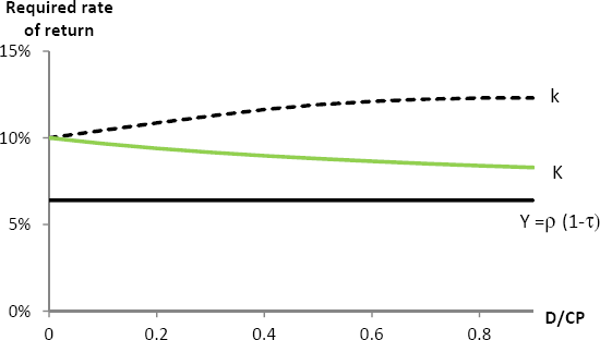
The company value is a product of discounting the cash flow that is available at rate K. Since debt is less risky, it is less expensive than equity. Thus, any moderate increase in debt decreases the WACC to the extent that a cheaper resource (debt) is substituted for a more expensive resource (equity). Having said this, any increase in debt in the weight of financing increases the risk of the shareholder passing it on to the cost of equity, which will cancel part of the decrease in total financial cost. In addition, at a certain level of debt owed, the cost also increases due to the increase of risk. The operation can be repeated until the requirement for the rate of return on equity is so high that it cancels out the positive effect of additional debt. At this level of financial leverage, the company has reached its optimal capital structure, as it has the lowest possible WACC (or cost of funding) and therefore the highest economic asset value.
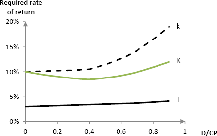
Figure 1.1. Optimal weighted average cost of capital according to the traditional approach
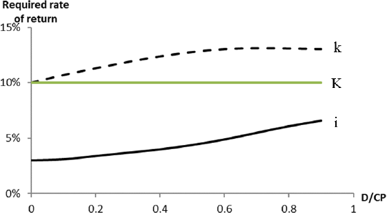
According to the theory of market equilibrium, in the absence of taxation, the enterprise value of two identical companies with different financial structures is the same. This is because investors can reproduce financial transactions at their level without additional cost and risk. In other words, when undertaking a valuation of the company, they are indifferent to any financial construction. Modigliani and Miller (1958) affirm that arbitrations made by investors imply that there cannot be an ideal liability structure in a market that is in equilibrium.
When i increases, the rhythm at which k progresses will slow down, such that K remains constant: stakeholders are relieved of part of the risk of the company that is passed on to the creditors as soon as the amount of debt becomes significant. In a market in equilibrium, the increase in expected profitability linked to the leverage effect and the increase in risk offset each other so that the value of the share remains the same. The increase in the level of debt that a company has increases the risk of the shareholder as well as the profitability that they require. This is so that ultimately the wealth of shareholders does not change. The value of debt comes down to the exact price that has to be paid for equity. In other words, one should not pay the company twice by buying the shares at the cost of the economic asset and then paying off the debts. Asset value is the same whether it is financed by debt, equity or both. The weighted average cost of capital of the company is independent of its two sources of financing. Debt and equity will adjust according to any change in financial structure. Indeed, increasing debt does not make the cost of capital decrease. On the contrary, debt increases the risk for shareholders and therefore the rate of return that they demand. The weighted average cost of capital is constant regardless of the financial structure.
From a mathematical perspective, the cost of capital of a company (independent of its financial structure) corresponds with the capitalization rate p of the expected operating profit of a company without debt and belonging to the same industrial risk class5. In other words, this leads us to consider that the enterprise value is akin to a perpetual growth rate of constant future operating results discounted at the rate ρ:
The cost of equity k corresponds to the financial profitability rf insofar as we can reason it ad infinitum. From there:
This theory does not explain the everyday reality for two key reasons. On the one hand, by conserving the same market logic, biases start to emerge. They explain why a business goes into debt and why it does not go beyond a certain threshold. The fundamental parameters are taxation and the costs of bankruptcy associated with excessive debt. On the other hand, there are interferences between the financial structure and the investment which can be explained above all by the divergent interests of different financial partners in terms of value creation and by the divergent personal situations in terms of access to certain information.
Modigliani and Miller (1963) perfected their theory by taking into account corporate tax. When we consider corporate tax, the result is that debt is favored over equity. In fact, financial expenses are deductible from the tax base on companies. The company’s creditors collect them without having already been taxed. However, dividends are not deductible. The shareholders receive them after tax payment. In a sense, deducted financial expenses can be seen as a state subsidy to the indebted company. So that they can benefit, it is enough for the expenses to be taxable, i.e. it is a beneficiary. If the company uses debt on a permanent basis, it will benefit from a tax economy that is considered at the level of the value of its economic asset:
where:
- – X: renumeration of capital providers to the indebted company;
- – X*: renumeration of capital providers to the company without debt;
- – VE: value of the assets of an indebted company;
- – VE*: value of the assets of a company without debt;
- – i: cost of debt;
- - ρ: cost of the capital of a company without debt;
- – VD: market value of debt;
- – VCP: market value of equity;
- – EBIT: operating result;
- – τ: corporate tax rate;
- – iVD: financial expenses;
- – iVDτ: tax reduction generated by the deductibility of financial expenses;
- – shareholders receive all of the corporate profits.
If we consider that the value of the assets corresponds to a perpetual annuity of future flows, then the flows of the company with no debt are discounted at the rate ρ, i.e. ![]() and the tax reduction if discounted at the cost of debt. Moreover:
and the tax reduction if discounted at the cost of debt. Moreover:
In the case of corporate tax, the value of the economic assets of a company with debt is equal to the value of the economic assets of a company without debt, increased by the present value of the related tax savings. This saving will only be effective if the profitability of the company is sufficient and it does not benefit from other exemptions (tax loss carryforwards, research tax credit, etc.). This is the basis of the APV method (adjusted present value), which separately recommends valuing economic assets by discounting cash flow and the value of the tax savings generated by financial expenses. The question then is to know the discount rate of the tax savings due to the tax deductibility of financial expenses. Modigliani and Miller advocate discounting the tax savings to the cost of debt.
This method is appropriate if one thinks that these tax savings are certain. Therefore, the value of the tax savings is equal to the value of the debt multiplied by the tax rate. On the other hand, it is commendable to think that the company will not be forever in debt, being the receiving party and taxed at the same rate. In this way, it is quite conceivable to discount the tax savings to the cost of equity, especially since it goes to the shareholder.
As a result, the adjusted cost of capital is first obtained by determining the cost of equity:
Recalling that the enterprise value VE* corresponds to a perpetual annuity of operating results (constant in the future) discounted at ρ or at the enterprise value VE minus the tax savings linked to the debt, we have:
And so, the cost of capital K equals:
The cost of capital thus is not affected by an increase in the cost of debt because the formula for the adjusted cost of capital does not contain i. In addition, Modigliani and Miller’s formula for the cost of capital expresses that an increase in the cost of debt i leads to a decrease in the cost of equity k.
The increase in debt burden in finance can be translated into a fall in the cost of capital. Therefore, the increase in debt burden results in an increase in enterprise value. The difference between the enterprise value of the company in debt and the enterprise value of the company not in debt corresponds to the value of the tax-saving perpetual annuity generated by the tax deductibility of financial expenses. In other words, the increase in debt only has the effect of increasing the value of tax credit (the change in the financial structure, as it has no impact on the value of industrial assets).
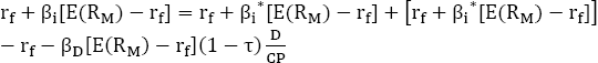
Hamada (1972) is influenced by the work of Modigliani and Miller when defining the equation of unlevered beta of a share. Starting from the cost of equity:
The CAPM equation is used, while assuming that the company is in debt at the risk-free rate (in this case i = rf):
Assuming the firm is in debt above the risk-free rate, CAPM is applied to the debt using the βD debt beta:
However, the costs of bankruptcy are the first limitation to this reasoning. Indeed, a company that has recurrent debt runs the risk of no longer being able to meet its commitments. If this is the case, the company files for bankruptcy, which theoretically qualifies as a reallocation of assets for productivity purposes. For an investor with a perfectly diversified portfolio, bankruptcy is seen as a mechanism for reallocating resources. The cost is therefore zero. However, in practice, markets do not work perfectly. Bankruptcy has a real cost because of its very nature. The decrease in enterprise value resulting from the inclusion of the costs of bankruptcy has been studied in particular by Molina (2005), Almeida (2007) and Bae (2011). The judicial liquidation of a company generates:
– direct costs: severance pay, attorney fees, legal costs, shareholder efforts to obtain a liquidation bonus, etc.;
– indirect costs: canceled orders (for fear that they won’t be honored), reduction in supplier credits (for fear of never being paid back), impact on productivity (strikes), inability to obtain funding, etc.
From this perspective, the bankruptcy of a company can be perceived as the refusal of shareholders to offer additional funds. They consider their previous bets to be lost. Shareholders effectively hand the company over to its creditors who thus become the new stakeholders. Creditors bear the full cost of the company’s demise, which further reduces the possibility of debts being paid back. Even though they don’t go as far as bankruptcy, the company with great debt faces the costs of dysfunction which penalize its value: a reduction of the cost of research and development, maintenance, training or marketing (in order to meet the debt deadlines), difficulty in finding new resources to finance profitable projects, demotivation of some of the staff members, etc.
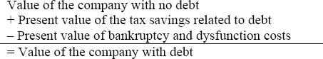
Due to tax deductibility, tax can create value. A business with debt may be worth more than a business with no debt. This point cannot be overstated for two main reasons. On the one hand, in times of crisis, excessive debt leads tax advantage to disappear (the company does not make enough profits). On the other hand, it can make dysfunction and bankruptcy costs emerge. The value of a company with debt can thus be broken down as follows:
The above reasoning can also be broken down in terms of the weighted average cost of capital. That is to say, when the company goes into debt, the cost of capital will be reduced thanks to the tax savings on interest. But when the company approaches bankruptcy, the costs of bankruptcy are factored into the rate of return demanded by investors. Paradoxically, we can uncover the traditional theory which advocates controlled debt. The optimal theoretical debt ratio is achieved when the present value of the tax savings due to additional debt is just offset by the increase in the present value of bankruptcy and dysfunction costs.
Investor taxation is the second limit to the reasoning. Miller (1977) echoes the 1958 conclusions from Modigliani concerning the lack of an optimal financial structure. In his theory, taxation is taken into account both at the level of the company and at the level of the investor. Miller argues that the effect of income tax cancels out that of corporate taxes so that the value of an economic asset is the same, regardless of the liability structure that finances it. The author observes that in general, investors are taxed more personally on debt income than on equity income. In other words, the tax advantage of debt at the corporate level is thwarted by the tax advantage of equity at the investor level. There is therefore no one source of funding that prevails over another:
and:
and:
where:
- – rf: risk-free rate;
- – ts: corporate tax rate;
- – ta: tax rate (legal persons) on the remuneration of shares;
- – to: tax rate (legal persons) on the renumeration of bonds.
The value of assets corresponds to a perpetual annuity of future cash flows. Therefore, the flows of the company without debt are discounted at the rate ρ and the flows generated by the debt are discounted at the risk-free rate rf. So:
Let VD’ be the capitalized value of debt for lenders:
And let G’ be the possible gain due to debt:
Therefore, if (1- to) = (1- ts) (1- ta), then G’= 0.
Factoring in investor income tax can reduce the debt benefit. Ultimately, it should be kept in mind that from this set of controversies, taxation is an essential parameter in absolute terms, but that it is unlikely that it serves to fully explain the financial structure of companies. What is more, the cost of debt per se may not be sufficient to explain a business’s choice as to whether or not to take out a loan. Indeed, the theory of markets in equilibrium starts from the affirmation that the company is a single player. Therefore, it ignores any conflicts that may arise between different stakeholders within the company as they may pursue different or even opposing goals. In this context, taking out debt can be seen more as a signal, beyond the financial considerations that are implied.
1.2.3. Theories of organizations
Signaling theory maintains that company executives have more information than funders and are better able to forecast future cash flows of the business. Thus, any signal emitted to show that flows are better than expected or that the risk is lower than expected enables the creation of value for the investor. In order for the signal to be credible, it must have its own sanction if it is proved to be wrong. Debt is seen as an indicator of the good health of a company since the manager of an underperforming company cannot go into debt. It reflects the manager’s desire to improve the financial performance of their company in order to generate the cash flows necessary to service the new debt. Synonymous with a market that bears good news, the loan generates a rise in stock prices. Ross (1977), Blazenko (1987), John (1987) and Narayanan (1988) have notably studied the role of debt as a signal given to the market on the financial health of companies. Indeed, the managers of a company whose debt is increasing signal to the market that they know the company’s status, that it is favorable and that the performance of the company will by consequence allow them to pay additional financial charges and repay this new debt without difficulty. And so, perhaps a signal does not tell us about the financial structure of a company, but rather its ability to transform. On the other hand, announcing an increase in capital leads to a drop in the share price. Indeed, directors do not carry out capital increases when the value appears to them to be undervalued (so as to not place their current shareholders in an unfavorable situation). If there is an unjustified increase in capital, the investor will deduce that the stock price is overvalued and that is why the current shareholders accept the emergence of shares. It is therefore evident that if a director sells their stake in a company, it is a negative signal. This means that they have internal information; that the value of future cash flows, taking into account the risk, is lower than the price at which they can negotiate their participation in the company. Conversely, any strengthening of their participation in the company, especially if it is financed by debt, will be a very positive signal for the market.
The preference theory or pecking order theory, initially presented by Myers and Majluf (1984), justifies the prioritization of funding methods. It assumes that managers choose the sources of finance with the lowest intermediation costs and agency costs. First, companies favor self-financing, i.e. internal financing. It does not require the submission of a file or any negotiation with third parties. In addition, dividend payment targets are tailored according to their investment opportunities. Then, depending on the year, if the results and opportunities are variable, companies use their cash flow. If the financing needs of investments exceed the amount of self-financing, companies resort to external financing. They first choose to issue low-risk debt, i.e. with guarantees for lenders. Likewise, if companies cannot call on traditional debt, they issue debt securities (from the less risky to the riskier). Finally, if the sources cited above prove to be insufficient, companies issue shares and carry out capital increases.
Agency theory takes place in a context of information asymmetry. The agency relation is a contract by which one person (the principal) appoints another person (the agent) to perform certain tasks. This contract implies that the principal delegates part of their decision-making authority to the agent. This relationship is problematic since the interests of the two parties are different. This produces a number of costs that are necessary for executives, for example, to behave in the best interests of the shareholders who appointed them. Agency theory is an attempt to draw a parallel between financial theory and the theory of organizations.
Agency costs can be due to debt. Indeed, in the situation of nearly reaching bankruptcy, a company with debt may accept risky, unprofitable projects (the net present value or NPV is negative), which reduces its value. This practice implies an increase in the value of equity at the expense of that of debt. Shareholders exclude the capital increase for fear of abandoning their contribution to creditors. However, this recapitalization makes it possible to carry out profitable projects. In this case, the agency costs represent the shortfall resulting from rejecting the project for lack of funding. Managers tend to make decisions in favor of the shareholders. These decisions may take the form of company-funded gifts or restrictions on the research and development budget (in order to optimize the distribution of dividends). These practices weaken the competitiveness of the firm and its ability to generate the cash flows that can be used to repay debt. As a result, lenders increase their requirements (agency costs) and insert protection clauses in their contracts. Smith and Warner (1979) have studied the role of these clauses which protect creditors from deviant behavior by shareholders.
Agency costs of equity are the result of disagreements between providers of capital and managers. They relate to companies with a large number of shareholders, which leads to a disconnect between the ownership and the management of the firm. These conflicts, studied by Jensen and Meckling (1976), are due to decisions taken by managers to the detriment of stakeholders. This may be excessive compensation and the allocation of benefits in kind, or inefficient use of surplus cash, instead of increasing the distribution of dividends. This results in the acquisition of marketable securities, whose NPV is equal to 0, that the shareholders could have bought if the company had distributed more dividends or by the acquisition of firms whose activity is not controlled by the company, with the initial aim of diversifying assets. In these cases, the enterprise value falls due to negative NPVs. This decrease corresponds to the agency costs of equity. As Charreaux (1997) explains, shareholders cannot control the deviant behavior of the leaders they have appointed. However, by resorting to debt, which can increase the risk of a company becoming bankrupt, the intention is to support the motivation of managers to make optimal decisions for the company and therefore for its shareholders.
The manager who is not a shareholder seeks to avoid debt which increases the company risk (increase in the breakeven point, financial costs and repayment deadlines that need to be respected) and therefore its own risk (as their income mainly comes from the company). As a precaution, they’ll tend to want to accumulate liquidity in the company rather than invest it in risky projects. This behavior is not in the shareholder’s interest, as they diversify their assets and perceive the state of being in debt as a stimulus for the manager, and so is encouraged to do their best to free up the cash flow available for the payment of financial expenses and to meet repayment deadlines. In other words, shareholders have an interest in debt to put management under pressure and thereby solve agency problems. The explicit cost of debt constitutes a powerful force impacting the company’s management team. Insofar as the parameters of debt are reflected in the company’s cash flow while financing via equity results in capital gains or losses at shareholder level, managers have all the more interest in the success of their investments as they are financed by debt. From here, questioning the theory of markets in equilibrium entails a second degree of questioning: the mode of finance influences the choice of investments to the extent that the different forms of finance do not give the same incentives to the business leaders. This means in turn that a company with debt would be more flexible and react faster than a company that is not in debt. The hypothesis has been empirically verified by Ofek (1993). He argues that companies that are listed in the US react (go bankrupt, cut dividends, experience layoffs, etc.) even faster to being in a lot of debt than when they are in a situation of crisis. When it preserves a balanced financial structure, debt is thus one of the modes of internal control that shareholders would choose when it comes to managers6 .
In this context, the exercise of business valuation is paramount for each of the stakeholders. Indeed, insofar as a company can buy and be bought, its valuation is of particular interest to investors who look to justify their decision to enter, lend or exit the share, with the manager enabling him/her to position the structure in relation to his/her peers, with the objective of adjusting their management. Therefore, considering the potential value of the company, the market will facilitate the development of financing.
1.3. Valuation measures and follow-up measures
Valuation consists of economically valuing the equity of a company. They can be valued directly or indirectly, i.e. by characterizing the overall value of the company and then deducting the amount of net debt from it in particular. There are three traditional methods.
The comparables method seeks to compare companies or assets of the same nature by focusing on forecasts of aggregates of the income statement and, possibly, of the short-term balance sheet (one or two years of forecast data are necessary as well as aggregates from the last fiscal year). Equity is thus valued by stock market or transactional comparisons.
When the development prospects are considered in the medium or long term, the method of discounted cash flow suggests calculating an intrinsic value of the target company. It results from the calculation of normalized future cash flows from operating income, thus excluding financial expenses, exceptional items and the payment of dividends. Discounting is based on the weighted average cost of capital (WACC). This incorporates the cost of equity and debt found in the CAPM. The value of equity is ultimately obtained by subtracting the value of net debt in particular.
Finally, the proprietary approach evaluates the company as a sum of its assets discounted from net debt. When setting up holding companies, the valuation of revalued net assets recommends restating the equity of hypothetical assets and liabilities before adding unrealized capital gains to them and subtracting unrealized capital losses. In the case of conglomerates, the estimated net assets seek to define, for each branch of activity, an enterprise value obtained by carrying out the assessment presented above. The sum of the various values corresponds to the enterprise value of the conglomerate from which the consolidated net financial debt is deducted to estimate the value of equity. After having evaluated the target, the acquisition can take place on condition that the financing processes have been completed and that the initiator’s earnings per share have been assessed, possibly to include the synergies generated by the acquisition.
1.3.1. Evaluation by comparative approach
Valuation by stock market comparisons is a method used to determine an objective stock market price of a company and in the context of a public offer when the offer price is presented. It is based on forecasts of financial aggregates. The company is valued for a multiple of its earning capacity, and the markets in equilibrium justify comparisons. This approach is holistic, focusing not on the value of operating assets and liabilities, but on the profitability of their use. The multiple becomes higher as the growth prospects become stronger. The sector of activity is slow risk, and the interest rate charged is low. The valuation of a company is carried out on the basis of a repository of companies that present the same industrial risk. For each of them, multiples of the income statement aggregates are calculated.
This is done by establishing the enterprise value of each company in the sample and relating it to the aggregate in question. Then, an average is taken for each category of multiples. The sector multiples formed from there are applied to the corresponding aggregate from the company that is under valuation. The various corporate values that are then defined are eventually restated, which results in economic values of equity. Depending on the financial specificities of the sector, the relevance of certain multiples will be justified. In addition, these multiples may be taken from a sample of companies that have recently been sold, and for which an equity value has been expressed. Therefore, a company’s shares will be valued using the first type of sample if there is no change in control to be noted and a company’s equity will be valued using the second type of sample, in case of a change in control. Using the share price to calculate the market multiples provides a “minority” value; the transaction multiples result in “majority” values because they include a control premium. There are two categories of multiples: those that establish enterprise value (multiples of aggregates before financial charges) and those establishing equity (multiples of aggregates after financial charges). Enterprise value EV is the economic value of operating assets. Since the balance sheet is in equilibrium:
where
- – MC: market capitalization;
- – MI: minority interests;
- – ND: net financial debt;
- – FA: financial assets.
Enterprise value therefore corresponds to the market value of the industrial and commercial tool. Fixed assets are excluded from this concept insofar as this enterprise value is intended to be compared with sales, gross operating surplus and operating income which do not include financial results. In addition, when restating the enterprise value that makes it possible to economically valuate the shareholders’ equity, net debt is notably subtracted, i.e. the financial debt to which investment securities and liquid assets are added. It is therefore necessary to add, during this last step, the financial fixed assets which differ from investment securities only in terms of where they are used. For its part, the net financial debt is made up of all short-, medium- and long-term financial debts, from the value of hedging instruments minus cash flow assets (liquid assets and transferable securities). Theoretically, the value of net debt preserves its market value, i.e. it is equal to the value of future flows to be paid (interest and capital) discounted at the market cost of the debt at which we can subtract the market value of financial investments. We can also use the market value of debts listed and/or traded within an over-the-counter market (bonds, syndications, credit derivatives or CDS). In practice, the market value is often equal to the carrying value (Le Fur and Quiry 2004). The two values are significantly different when:
- – the company is indebted at a fixed rate by means of a swap and the interest rates have fluctuated in the meantime;
- – the solvency has undergone a significant change after the company has contracted a debt without the interest having been adjusted;
- – the nominal rate of the debt has been artificially reduced by the addition of warrants (or other detachable products after the issue).
Finally, market capitalization corresponds to the economic value of equity. If the company is listed, it is equal to the number of shares multiplied by the market price7.
Throughout this work, the provisions have not undergone any restatement for the following reasons:
- – differences in accounting standards IFRS and US GAAP in particular lead to significant discrepancies8;
- – in practice, analysts can assume that they are integrated into the result (thus in equity);
- – theoretically, provision for pensions can be assimilated to a financial debt towards employees (Le Fur and Quiry 2003). In practice, analysts can reintegrate it directly into net debt. It is readjusted each year in order to take into account when it is updated9. It is similar to a zero coupon bond for which each year the company recognizes an interest charge payable only at the end date. However, if the retirement provision is taken into account when calculating the enterprise value, it is essential to ensure that the EBITDA and the operating profit do not include the fraction of the allowance that corresponds to the passing of time.
And so, the multiple of turnover (TO) shows that the value of operating assets is equivalent to a certain number of times the turnover:
This multiple is of particular interest for a sample which displays a normative and relatively low economic profitability. Otherwise, the results obtained will be heterogeneous. In addition, this multiple makes sense for SMEs for whom turnover is much more indicative of real profitability than the net result published, where transactions are numerous. Finally, this multiple is to be avoided when comparable companies are profitable because in this case it will tend to overvalue the company. In the equation, by replacing the TO by the EBITDA and by the EBIT, we have:
The multiple of operating profit makes it possible to enhance the profitability of the company by excluding non-recurring items.
The multiple of gross operating surplus eliminates any significant differences in investment and related repayment choices. The multiple is particularly suited to capital-intensive industries. However, despite the choice of depreciation arrangements, this multiple loses its usefulness in the case where the margin levels of the sample are different.
Companies with low margins are then overvalued, while the opposite effect occurs for those with high margins. P/E is the ratio of the share price to earnings per share. It corresponds to a direct approach10:
Income generated by financial assets is included in net income. In addition, the net result is “shared within the group”. This is the reason why no restatement of financial assets and minority interests is to be made.
In practice, net income is restated for non-recurring items and goodwill impairment in order to facilitate an analysis of recurring earning capacity. Indirectly, this multiple based on an aggregate after financial expenses values the financial structure of the company. Thus, if the sample’s debt levels are disparate, the valuation may be skewed. This is the reason why, in order to break away from heterogeneous financial structures, the multiple of operating income and, to a lesser extent, that of gross operating surplus are used more.
Based on the estimates of analysts, it is customary to calculate the multiples of comparables on the forecast values of the income statements of companies in the benchmark and the target, always considering the last published financial year. The question then arises as to whether the corporate values should be current (i.e. corresponding to the last published financial year) or whether they can also be forecast. Indeed, the second method fully integrates the investment and financing policy of the company (Le Fur and Quiry 2007). In other words, it seems theoretically irrational to consider, in the multiple of operating income, the investments made in year N+1 (through estimated depreciation) without including in the calculation of the financing linked to these (through “new” equity and/or “new” debt).
By incorporating the notion of forecast value, this method would be granted the ability to differentiate between company multiples with distinct investment and growth profiles. However, the practice tends to go against this reasoning due to the fact that if we were to calculate the value of asset N+1 of the company, we can estimate the net debt N+1. It is, however, impossible to guess the market capitalization N+1. We could propose to capitalize the value of equity N at the cost of capital minus the rate of return.
However, empirically, this method is not used because the market incorporates known future data, through the share price and therefore the market capitalization. Furthermore, the operating profit multiple could be biased if the company is largely financed by debt: the multiple would be unfairly very high. Finally, the other elements allowing the transition from enterprise value to that of equity are most often considered constant because it is difficult to predict. Therefore:
- – to value a company in year N+1, it is advisable to keep the same value of the economic assets of the comparable company as for the year N11. In any case, the market value of the latter at the valuation date results from the anticipation of how its future operating balances will evolve;
- – if a comparable company has a strong investment policy, it is better to exclude it from the sample rather than wanting to wrongly improve the method of evaluating comparables.
The different economic values of equity allow us to compare the company under valuation to its competitors:
- – if the value of equity on the basis of the EBITDA multiple is higher than that of turnover, the assessment is more favorable for the company subject to the study since its EBITDA margin is greater than those of its competitors. This point can be verified by comparing the EBITDA margins of the sector with that of the company to be valued;
- – if the value of equity on the basis of the multiple of EBIT is higher than that of EBITDA, the valuation is more favorable for the company subject to the study because it has less depreciation and provisions than its competitors. This may reflect a weak investment policy that may reflect a problem of competitiveness;
- – if the value of equity based on P/E is greater than that based on EBIT, the valuation is more favorable for the company subject to the study because the leverage effect is used more intensively.
In order to use the transaction multiple method, the sample is built from the information available on transactions observed in the near past in the same sector of activity (among listed and unlisted companies) and from the moment when a change of control has been observed. The acquirer has logically paid an offer price which, in this case, appears as enterprise value.
This price paid incorporates a control premium (of the order of 20–25% of the company’s value) which is essential to take possession of the target and which results from a valuation of a share of the anticipated synergies. For each of the companies in the repository, we determine the multiple of turnover, EBITDA, EBIT, P/E of the last financial year closed on the date of the transaction. In other terms, for a transaction carried out in year N, we consider the aggregates of year N-1. For the numerator, the transaction amount replaces the market capitalization. Finally, each average transactional multiple obtained is applied to the homologous aggregate of the company under valuation.
By way of illustration, it was decided that the market comparables method would be applied to value the Royal Dutch Shell company, using a benchmark of companies from the oil industry. Royal Dutch Shell is an Anglo-Dutch company that specializes in energy and petrochemicals. The core business function is to refine and distribute petroleum and natural gas (90% of its turnover at the end of 2013).
The group owns more than 30 refineries and a network of around 44,000 service stations around the world. Around 40% of its activity is carried out in Europe, 35% in Asia-Oceania-Africa and around 25% on the American continent.
On December 5, 2014 (its valuation data), Royal Dutch Shell shares were listed at €27.26 at the opening of the Amsterdam Stock Exchange (AEX Index). Although of different sizes, the companies selected to constitute a reliable repository were Exxon Mobil, Chevron, Conoco Phillips, Petrobras and Total SA.
For the sake of homogenization, the amounts processed – namely the market capitalizations and the data of the balance sheet and income statement aggregates (realized or forecasted) – are expressed in dollars and then, to proceed with the valuation of the share, are quoted in euros, and so a conversion into the European currency is carried out. Moreover, on December 5, 2014, the EUR/USD parity was 1.2282 (parity applied to the benchmark aggregates of Total SA) and the USD/BRL parity was 2.5894 (parity applied to the benchmark aggregates of Petrobras).
Company aggregates for 2013 are taken from financial statements published by oil companies. The 2014 and 2015 forecast data and market capitalization are taken from zonebourse.com.
The multiples of the aggregates of the companies and the average multiples, assimilated to the sector multiples, are shown in Table 1.2.
Applying the average multiples to the corresponding aggregates for Shell finish the valuation12.
The results of this valuation approach are represented in Figure 1.4.
Table 1.1. Financial aggregates of the companies in the framework (amounts in millions of $)
| Market capitalization (05/12/14) | Net debt | Financial assets | Minority interests | Enterprise value | |
| Exxon Mobil | 397,283 | 18,055 | 36,328 | 6,482 | 385,492 |
| Chevron | 209,591 | 3,915 | 25,502 | 1,314 | 189,318 |
| Conoco Phillips | 83,517 | 15,416 | 23,907 | 402 | 75,428 |
| Petrobras | 59,433 | 94,579 | 6,666 | 596 | 147,942 |
| Total SA | 131,990 | 21,027 | 18,182 | 2,802 | 137,636 |
| Sales | EBITDA | EBIT | Net income | |||||||||
| 2013 | 2014* | 2015* | 2013 | 2014* | 2015* | 2013 | 2014* | 2015* | 2013 | 2014* | 2015* | |
| Exxon Mobil | 438,255 | 417,504 | 379,124 | 74,902 | 72,980 | 63,016 | 57,720 | 54,835 | 43,024 | 32,580 | 32,674 | 27,706 |
| Chevron | 228,848 | 214,418 | 184,158 | 63,154 | 47,550 | 42,703 | 48,968 | 31,341 | 24,313 | 21,423 | 19,618 | 16,974 |
| Conoco Phillips | 58,248 | 56,635 | 54,194 | 23,455 | 21,911 | 20,221 | 14,446 | 12,669 | 9,996 | 9,156 | 7,982 | 6,371 |
| Petrobras | 141,462 | 154,934 | 164,128 | 29,426 | 32,204 | 39,958 | 16,083 | 17,110 | 22,208 | 10,832 | 9,464 | 13,121 |
| Total SA | 232,795 | 214,493 | 200,870 | 35,034 | 35,408 | 35,037 | 24,915 | 22,754 | 21,205 | 10,637 | 12,720 | 13,000 |
*Forecasts zonebourse.com
Table 1.2. Stock market repository of repository companies
| xSales | xEBITDA | xEBIT | P/E | |||||||||
| 2013 | 2014* | 2015* | 2013 | 2014* | 2015* | 2013 | 2014* | 2015* | 2013 | 2014* | 2015* | |
| Exxon Mobil | 0.88 | 0.92 | 1.02 | 5.1 | 5.3 | 6.1 | 6.7 | 7.0 | 9.0 | 12.2 | 12.2 | 14.3 |
| Chevron | 0.83 | 0.88 | 1.03 | 3.0 | 4.0 | 4.4 | 3.9 | 6.0 | 7.8 | 9.8 | 10.7 | 12.3 |
| Conoco Phillips | 1.29 | 1.33 | 1.39 | 3.2 | 3.4 | 3.7 | 5.2 | 6.0 | 7.5 | 9.1 | 10.5 | 13.1 |
| Petrobras | 1.05 | 0.95 | 0.90 | 5.0 | 4.6 | 3.7 | 9.2 | 8.6 | 6.7 | 5.5 | 6.3 | 4.5 |
| Total SA | 0.59 | 0.64 | 0.69 | 3.9 | 3.9 | 3.9 | 5.5 | 6.0 | 6.5 | 12.4 | 10.4 | 10.2 |
| Sector multiple | 0.93 | 0.95 | 1.00 | 4.1 | 4.2 | 4.4 | 6.1 | 6.7 | 7.5 | 9.8 | 10.0 | 10.9 |
*Forecasts zonebourse.com
The valuation by the multiple of EBITDA is lower than that resulting from the turnover, given the profitability differential between the sector and Shell, to the detriment of the Anglo-Dutch company. Its EBITDA margin is lower (about 13% for Shell vs. about 24% for the sector). The valuation resulting from the multiple of EBIT is in line with that which results from the multiple of EBIDTA, which comes from an equivalent proportion of depreciation and impairment between the sector and Shell. The valuation by the P/E is lower than that which came from the EBIT. The valuation could improve if the company had recourse to debt, provided that its economic profitability was greater than the cost of its debt. Therefore, it is necessary to exclude the valuation that results from the turnover multiples because the profitability differentials between Shell and its competitors are not taken into account: applying the turnover multiple will overvalue the share.
Table 1.3. Valuation of Royal Dutch Shell by stock market comparisons (amounts in millions of $)
| xSales | xEBITDA | |||||
| 2013 | 2014 | 2015 | 2013 | 2014 | 2015 | |
| SHELL Aggregate | 451,235 | 448,379 | 423,292 | 59,864 | 60,436 | 57,160 |
| SHELL EV | 418,643 | 424,583 | 425,257 | 243,244 | 256,093 | 250,494 |
| (Net debt 2013) | (34,866) | (34,866) | (34,866) | (34,866) | (34,866) | (34,866) |
| Financial assets 2013 | 39,328 | 39,328 | 39,328 | 39,328 | 39,328 | 39,328 |
| (Minority interests 2013) | (1,101) | (1,101) | (1,101) | (1,101) | (1,101) | (1,101) |
| Economic value of equity | 422,004 | 427,944 | 428,618 | 246,605 | 259,454 | 253,855 |
| Number of shares (millions) | 6,371 | 6,371 | 6,371 | 6,371 | 6,371 | 6,371 |
| Target share price ($) | 66.24 | 67.17 | 67.28 | 38.71 | 40.73 | 39.85 |
| Target share price (€) | 53.93 | 54.69 | 54.78 | 31.52 | 33.16 | 32.44 |
| xEBIT | P/E | |||||
| 2013 | 2014 | 2015 | 2013 | 2014 | 2015 | |
| SHELL Aggregate | 38,355 | 33,905 | 32,781 | 16,371 | 21,379 | 22,088 |
| SHELL EV | 233,881 | 228,654 | 245,496 | |||
| (Net debt 2013) | (34,866) | (34,866) | (34,866) | |||
| Financial assets 2013 | 39,328 | 39,328 | 39,328 | |||
| (Minority interests 2013) | (1,101) | (1,101) | (1,101) | |||
| Economic value of equity | 237,242 | 232,015 | 248,857 | 160,416 | 213,627 | 240,663 |
| Number of shares (millions) | 6,371 | 6,371 | 6,371 | 6,371 | 6,371 | 6,371 |
| Target share price ($) | 37.24 | 36.42 | 39.06 | 25.18 | 33.53 | 37.78 |
| Target share price (€) | 30.32 | 29.65 | 31.80 | 20.50 | 27.30 | 30.76 |

Figure 1.4. Summary of valuations by stock market comparisons of shares from Royal Dutch Shell (in €)
In addition, it is wise to rule out the valuation that results from the P/E to the extent that any leverage effect is taken into account in a context where financial structures are heterogeneous. Thus, market capitalizations, which are too disparate between Shell’s competitors, do not constitute a relevant benchmark. The target price therefore corresponds to the average of the valuations that result from the EBITDA and EBIT multiples for 2013, 2014 and 2015. Based on the market comparables method and the price on December 5, 2014 (€27.26), the share appears to be undervalued. According to the study carried out, in the medium term, the upside potential may lead the share to list €31.48, i.e. an equity valuation of €200,569 million or $246,338 million (market capitalization on December 5, 2014 is €175,569 million or $215,634 million).
The method used in this application, based on short- and medium-term forecasts, excludes the potential for business development and improvement of long-term profitability. The discounted cash flow (DCF) approach allows us to assess the economic value of operating assets over a much broader space and timeframe using a financing plan. In other words, it is about finding the enterprise value that comes from the sum of the discounted future free cash flows (FCF) generated by the activity of the company to be valued.
1.3.2. Flow assessment
The economic value of equity can be obtained following two methods. The first consists of considering that the income of a company’s shareholder is made up of dividends received and the market value of the shares that are on resale. Therefore, enterprise value should be based on the sum of the future dividend flows payable by the enterprise and the market value of the stocks at the end of the expected space–time horizon. The second method for obtaining the economic value of equity consists first of estimating the value of the economic asset before subtracting from it the amount of net debt as well as minority interests, before adding the value of fixed assets.
1.3.2.1. Dividend discount model
Assuming that the expected space–time frame is infinite, the dividend discount model will not incorporate capital gains since it does not affect the valuation of the share. This notion is thus formalized and an intrinsic value of the company is defined as the present value of future dividends discounted at the cost of equity. Thus, we have:
where:
- – Vt: intrinsic value of equity in time t;
- – Dt: dividends expected at the period of time t (with information being available at the time t-1);
- – k: cost of equity given the CAPM formula.
Let’s assume that the dividends have an annual growth rate g:
And so:
Knowing that:
because if ![]() .
.
Here:
We therefore have the formula expressed by Gordon and Shapiro (1959):
Applied when the company to be valued operates in a mature sector with good visibility (public services, real estate companies, etc.) with a high dividend distribution rate, this method nevertheless has the weakness of not taking into account the organic growth via resources set aside. In practice, many younger companies with high growth potential tend to keep most of their profits or, with a finite forecast horizon, they have no intention of paying dividends. Therefore, the market values of this type of company are larger than those found through the Gordon and Shapiro equation. What is more, according to Modigliani and Miller (1963), the value of a share is not linked to the date that the dividends were paid. It is not uncommon to come across a company that is borrowing funds in the markets in order to be able to remunerate its shareholders, this all being without any apparent link with operating activities or with an investment policy which has created value. The DDM thus focuses on distributing money to shareholders by assuming a consistent distribution without necessarily having any link to the creation of value.
1.3.2.2. Discounted cash flow model
The economic value of operating assets results from calculating the enterprise value. It corresponds to the sum of the discounted future free cash flows that have been generated. Subsequently, the net debt and minority interests are subtracted from it, then financial fixed assets are added to it. We can then obtain the economic value of the equity. In order to find the value of the operating economic asset in the first place, we may apply the technique of choosing the investments that are based on some sort of reasoning:
– in terms of cash flow and not in terms of accounting results. This makes it possible to take into account the variation in the working capital requirement, i.e. the impact of payment delays. In addition, depreciation is calculated according to tax and accounting rules and does not always correspond to an economic reality. An amount only costs or yields at the very time of disbursement or collection, regardless of the treatment given to it. Beyond that, the reasoning is carried out more in terms of opportunity than accounting. Indeed, the account or historical value is of no interest except for tax purposes to know the tax paid on capital gains or tax credits obtained in the event of book value losses. The asset has value, i.e. it corresponds to the acquisition price in the event of investment and to the resale price in the event of divestment;
– in terms of flows induced by operation and investment only. Thus, financing flows are discarded because the cash flows are intended to be discounted at the weighted average cost of capital; the purpose of the calculation being to compare the profitability of investments with the cost of financing. This eliminates financial charges, capital repayments and dividend payments;
– in matters of taxation. Depreciation results in tax savings. The results of the investments are taxed. Depending on the type of investment, the company may benefit from tax credits, allowances, subsidies, etc.
Therefore, the FCF17 are determined using the taxed operating income (tax is a disbursement). Depreciation (net allocations of reversals), which reduce operating income without reducing cash flow, must be reinstated. In addition, in order to neutralize the receivable income not yet collected and the disbursable expenses not yet disbursed, the change in WCR must be deducted. Finally, net investments of divestments that are not taken into account in the aggregates mentioned constitute disbursements. They must be deducted.
The value of operational assets V equal to the sum of the discounted future FCF is written as so:
with:
This method therefore involves determining the cash flows up to infinity. To achieve this, updated forecasts are made over an explicit horizon (5–7 years or even 20–30 years in utilities services) and beyond this horizon, a terminal value is considered18. The duration that characterizes the explicit horizon must correspond to the time during which the company will live on its current momentum. If it is too short, the valuation will rely excessively on the terminal value. If it is too long, the valuation will be the subject of a simple theoretical extrapolation. In addition, a growth rate g is applied to the final value. At first glance, it is difficult to estimate the terminal value since the date from which it is defined is synonymous with presumption when making forecasts. Therefore, analysts consider that at the end of the explicit horizon, the company has reached its maturity phase. Using the Gordon and Shapiro formula, the most commonly used terminal value is derived from an infinite growth rate g applied to a normative flow. The way it can be characterized is the consequence of the investment policy and the evolution of the company’s working capital needs. Moreover, it may not be equal to the last flow of the explicit horizon if the activity sector is cyclical because in this case, it would correspond to an average flow generated by the company up to infinity, while the growth forecast for this last year of the business plan would significantly differ from g.
However, it is necessary to question the sustainability of market growth and the economic profitability of the company. It would be unfounded to assume a growth rate g that is significantly higher than what analysts expect for long-term genuine growth (net after inflation). This would mean that the company to be valued would gain more and more importance in the economy over time. The “diminishing rent” model proposes to converge the expected economic profitability of the company towards the cost of capital. This model of cash flow fade makes it possible to create a moment at which the economic profitability deteriorates until it becomes equal to the weighted average cost of capital. This moment would come to pass between the end of the business plan and the terminal value. This can be explained by the decline in margins or by the decline in turnover of economic assets. At the end of the horizon, the final value is equal to the economic asset for its book value. Finally, this model can be applied to a company that is destroying value. In this case, the use of cash flow fade is justified, by assuming that the industry in question cannot remain in the same situation indefinitely. The structural changes, brought about sooner or later by bankruptcies or by market saturation, will make the flows of the company to be valued approach the cost of capital, allowing it to survive (thanks to the growth of economic profitability). Thus, several scenarios can be considered depending on whether we consider the point of view of the prospective buyer or the seller. Negotiations between the two parties will then make it possible to reconcile the valuations of the prices. In practice, the DCF method can be an appropriate dialogue tool. The rate used to discount FCF is the weighted average cost of capital (WACC), which is the weighted average cost of the company’s financial resources. It represents the minimum rate of return required by fund providers to finance the business. This situation results from the “fungibility” of the balance sheet. It is impossible to determine from a company’s accounts the financing of a given asset. Consequently, each asset is financed by equity E and by debt D; the weight of the first and the second in financing each asset corresponds to the weight of each resource in the economic balance sheet of the company. We then have:
where:
- – K: CMPC;
- – k: cost of equity;
- – i: cost of debt;
- – t: tax rate.
The economic value of the equity required to determine the WACC and therefore the discount rate is precisely what the DCF method should achieve. This is an iterative approach that loops through the value of equity. Approximating a listed company allows us to preserve market capitalization in the WACC formula. Equity value is the difference between EV enterprise value, net financial debt, minority interests, provisions to which financial fixed assets are added. Therefore, maximizing enterprise value through discounting future cash flows leads us to consider the possible existence of an optimal financial structure.
By way of illustration, it was decided that the DCF method would be applied to value the company Royal Dutch Shell. Table 1.4 presents the elements of the financing plan for the Anglo-Dutch company.
In order to extend the business plan from 2017, the assumptions are as follows:
– the growth rate of turnover is estimated at 3% by 2021. Consequently, from 2017 to 2021, there is a linear convergence between the growth rate of the last forecast year (2.2% in 2016) towards the last year of extension (3% in 2021);
– the EBITDA margin rate 2016 (14.1%), the allocations/turnover ratio in 2016(6.1%) and the corporate tax rate in 2016 (44%) are maintained from 2017;
– the amount of investments in 2021 is equal to the level of allocations planned for the same year ($29,941 million). This results from the assumptions that the company is fully mature by 2021, which then leads it to renew its stock of fixed assets at the rate of its allocations. And so, from 2017 to 2021, there is a linear convergence of the amount of investments for the last forecast year ($34,238 million in 2016) to the level of allocation of the last year of extension ($29,941 million in 2021);
– the WCR is considered to be normative. Consequently, the WCR/turnover ratio observed in 2013 (3.3%) is maintained from 2014 to 2021. From here, we deduce for each year the variation in WCR which comes with the reduction of free cash flows.
Table 1.4. Valuation by DCF of Royal Dutch Shell (amounts in millions $)
| Production | Sourced from zonebourse.com | Extension | |||||||
| 2013 | 2014 | 2015 | 2016 | 2017 | 2018 | 2019 | 2020 | 2021 | |
| Turnover | 451,235 | 448,379 | 423,292 | 432,800 | 443,174 | 454,465 | 466,729 | 480,027 | 494,428 |
| Growth rate | -0.6% | -5.6% | 2.2% | 2.4% | 2.5% | 2.7% | 2.8% | 3.0% | |
| EBITDA | 59,864 | 60,436 | 57,160 | 60,885 | 62,344 | 63,933 | 65,658 | 67,529 | 69,555 |
| EBITDA margin rate | 13.3% | 13.5% | 13.5% | 14.1% | 14.1% | 14.1% | 14.1% | 14.1% | 14.1% |
| (Depreciation allowances) | (21,509) | (26,531) | (24,379) | (26,209) | (26,837) | (27,521) | (28,264) | (29,069) | (29,941) |
| In % of TO (turnover) | -4.8% | -5.9% | -5.8% | -6.1% | -6.1% | -6.1% | -6.1% | -6.1% | -6.1% |
| EBIT | 38,355 | 33,905 | 32,781 | 34,676 | 35,507 | 36,412 | 37,394 | 38,460 | 39,614 |
| (Corporation tax) | (17,066) | (14,918) | (14,424) | (15,257) | (15,623) | (16,021) | (16,454) | (16,922) | (17,430) |
| Tax rate | 44.0% | 44.0% | 44.0% | 44.0% | 44.0% | 44.0% | 44.0% | 44.0% | |
| NOPAT | 21,289 | 18,987 | 18,357 | 19,419 | 19,884 | 20,391 | 20,941 | 21,537 | 22,184 |
| Depreciation allowances | 21,509 | 26,531 | 24,379 | 26,209 | 26,837 | 27,521 | 28,264 | 29,069 | 29,941 |
| (Net investments) | (40,146) | (33,495) | (33,726) | (34,238) | (33,379) | (32,519) | (31,660) | (30,800) | (29,941) |
| (DBFR) | (2,988) | 94 | 829 | (314) | (343) | (373) | (405) | (439) | (476) |
| FCF | (336) | 12,117 | 9,839 | 11,076 | 13,000 | 15,019 | 17,140 | 19,367 | 21,708 |
| Discount period | 1 | 2 | 3 | 4 | 5 | 6 | 7 | 8 | |
| Discounted FCF | 11,359 | 8,646 | 9,123 | 10,038 | 10,872 | 11,630 | 12,319 | 12,944 | |
| WCR | 14,904 | 14,810 | 13,981 | 14,295 | 14,638 | 15,011 | 15,416 | 15,855 | 16,331 |
| WCR/TO | 3.3% | 3.3% | 3.3% | 3.3% | 3.3% | 3.3% | 3.3% | 3.3% | 3.3% |
Table 1.5. Determining the weighted average cost of capital of Royal Dutch Shell
| Risk-free rate | 1.00% |
| Market risk premium | 5.74% |
| SHELL Beta | 1.08 |
| Cost of equity (k) | 7.22% |
| Cost of debt (i)... | |
| ... before tax | 4.37% |
| ... after tax | 2.45% |
| Discount rate (WACC = K) | 6.73% |
| Growth rate to infinity (g) | 3.00% |
In order to determine the discount rate:
– the risk-free rate (corresponding to the 10-year OAT rate) which was used is 1%19;
– the market risk premium was obtained by first constituting a benchmark, all sectors of activity combined, of about 300 companies listed on the CAC 40, AEX, DAX, FTSE 100, FTSE MIB, l’IBEX 35, PSI 20, Dow Jones, Nasdaq and Nikkei 225. Then, for each of the companies in the sample, the quotes at the opening of the stock market on December 5, 2014 were retrieved as well as the estimate of the next dividend paid and the beta of the share20. Assuming, on the other hand, an infinite growth rate of 3%, the risk premiums for each company were calculated according to the Gordon and Shapiro equation:
where:
– V0: share price i on December 5, 2014;
– D1: estimate of the next dividend paid linked to the share i;
– βi beta of share i;
– rf: risk-free rate;
– E(Ri) – rf: equity market risk premium of share i.
The market risk premium is therefore equal to the average of the 300 values thus calculated, i.e. 5.74%;
– the beta of the Royal Dutch Shell share was obtained by establishing a repository of companies belonging to the same sector of activity as the Anglo-Dutch company. The oil companies chosen are Exxon Mobil, Chevron, Conoco Phillips, Petrobras and Total SA. For each of them, the (indebted) beta of the shares was recovered as well as the net debt and market capitalization21. Then, for each of the companies in the benchmark, the debt-free beta was calculated using Hamada’s formula (1972):
| Beta | Net debt | Equity | Debt-free beta | |
| Exxon Mobil | 0.9 | 18,055 | 397,283 | 0.88 |
| Chevron | 1.15 | 3,915 | 209,591 | 1.14 |
| Conoco Phillips | 1.07 | 15,416 | 83,517 | 0.97 |
| Petrobras | 1.83 | 94,579 | 59,433 | 0.97 |
| Total SA | 1.11 | 21,027 | 131,990 | 1.02 |
The average debt-free beta (0.99) corresponds to the debt-free beta in the sector. Finally, the following is applied to the financial structure of Royal Dutch Shell:
The (re)indebted share of Royal Dutch Shell is at 1.08;
– the cost of equity (7.22%) is obtained by applying the CAPM formula;
– the cost of debt is determined according to the Standard & Poor’s debt rating guide. As of January 17, 2014, Shell bonds are rated according to the AA rating agency and the associated cost of debt is 4.37% before IS (i.e. 2.45% after tax);
– the FCF is discounted using the weighted average cost of capital (6.73%) by performing an iterative calculation of the WACC (closure on the desired value);
– the infinite growth rate (3%) is the assumed rate, in accordance with the assumption made in corporate and investment banks, and is in line with the method for determining the market risk premium.
The 2013 balance sheet shows a net financial debt of $34.9 billion. Enterprise value ($298.6 billion) is equal to the sum of discounted FCF over the business plan period ($86.7 billion) and the terminal value ($211.9 billion). The economic value of equity ($302 billion) is obtained by deducting new debt, minority interests and auditing financial assets to the enterprise value. Shell’s target price is thus $48.4 or €38.59 (the stock market price is €27.26 on the valuation date, December 5, 2014).
| Sum of DCFs 2014-2021 | 86,745 |
| Terminal value | 211,855 |
| Enterprise value | 298,600 |
| (Net debt) | (34,866) |
| Fixed assets | 39,328 |
| (Minority interests) | (1,101) |
| Equity | 301,961 |
| Number of shares (millions) | 6,371 |
| Target price ($) | 47.4 |
| Net result 2013 | 16,371 |
| Implied | 18 |
| Target price (€) | 38.59 |
Table 1.8. Sensitivity analysis of the value of Royal Dutch Shell at the risk-free rate and to infinite growth
| Risk-free rate | ||||||
| 1.0% | 1.5% | 2.0% | 2.5% | 3.0% | ||
| Growth rate g | 3% | 301,961 | 269,528 | 243,633 | 222,521 | 205,007 |
| 4% | 375,621 | 324,694 | 286,246 | 256,259 | 232,261 | |
| 5% | 515,810 | 420,578 | 355,472 | 308,274 | 272,563 | |
| 6% | 886,304 | 628,291 | 487,344 | 398,781 | 338,122 | |
Based on the discount rate and perpetual growth rate retained ad infinitum, the valuation is between $205 billion and $886 billion. The advantage of this method is to concretely translate the different assumptions and forecasts of buyers and sellers. A certain serenity is maintained in the face of periods of stock market overvaluation. It keeps economic performance grounded in reality. This method, satisfactory in theory, has three major drawbacks, however:
– is it very impacted by the assumptions and objectivity of the person who established it. Therefore, its results are very volatile. This is a rational method that can be biased;
– sometimes, it depends too much on the terminal value, to which the problem is ultimately transferred. Terminal value often explains 50% of the company’s value (Vernimmen 2012, p. 743). This can call into question its validity even though, sometimes, it is the only method applicable when the results are negative and the multiples are not applicable;
– it is not always easy to carry out a business plan over a sufficient period of time: the information is often lacking for the external analyst.
The two valuation methods discussed above are based, on the one hand, on a stock market analysis and, on the other hand, on what the asset portfolio would be worth in the future. A third valuation method is to intuitively consider that the business is worth what it owns in reality and instantly.
1.3.3. Valuation through propriety and mixed approaches
The propriety methods consist of valuing the assets, divisions or subsidiaries separately, by deducting the commitments of the company. The objective is to correct and reassess book values that are different from the actual values due to the consideration of accounting, tax and historical rules. This valuation method is particularly suitable for conglomerates or groups whose activities are diversified insofar as their accounts and financial projections must be the subject of separate analyses. In fact, the assets valued correspond to subsidiaries for their share of ownership or to branches of activity value separately using the multiples of DCF method. The holding’s net debt and the present value of the head office costs then decrease this sum. There are three types of asset values: market value, which represents the value of reselling an asset, the net asset value, which corresponds to the market value minus a discount linked to the need for a quick sale, and the use value, which represents the value of an asset within the operating process. Thus, since several perspectives are possible, the assessment must preserve the consistency of its approach (cessation of activity or continued operation). The value of a company with high asset value can bring about speculation and volatility insofar as the terminal value plays a very important part compared to intermediary flows, considering the DCF method. In other words, the industrial risk may be low, but it causes speculation for the value of resale. Therefore, this valuation method is useful for valuating SMEs with no strategic value or industrial assets for which a secondary market exists.
1.3.3.1. Revalued net assets
In order to define the revalued net asset, it is necessary to consider the account net asset which corresponds to the difference between the real assets (assets with a market value) and the real debts. Assets other than real assets are hypothetical assets, i.e. uncalled subscribed capital, start-up costs, research and development costs, bond redemption premiums and accrual-asset accounts (namely charges to be distributed, prepaid charges and rate differences on assets). Hypothetical debts (other than real debts) are accruals and deferred income (i.e. deferred revenues and unrealized foreign exchange)
Revalued net assets result from the difference between the economic value of real assets (generally greater than the net book value) and the economic value of real debts (commonly assimilated to their book value)NAV = economic value of real assets – real debts
The economic valuation of tangible assets does not mean that it is a matter of breaking down the value of each asset and then adding it up. It is the intrinsic overall value of the industrial and commercial tool that matters. In addition, the stocks of certain companies with a long production cycle may be subject to revaluation in the event of any capital gains noted. In this case, we must also take into account the impact of corporate tax. Finally, intangible assets are subject to specific valuation methods:
– business capital is assessed for SMEs on the basis of scales used by experts and courts as a percentage of turnover. For large groups, it is assessed by discounting the excess profit generated at the economic rate of return given a probable lifespan, depending on an attrition rate;
– trademarks and patients can be valued by considering advertising expenditure post tax.
In addition, a provisional balance sheet must not contain unrealized losses. However, unrealized losses or unrealized capital losses on certain assets must be deducted from the NAV:
where:
– UL: unrealized losses;
– UG: unrealized gains.
Taking tax into account implies adopting a certain approach to valuation:
– from a continuity point of view, the tax impact is neglected because the company does not intend to sell the assets that generate capital gains. Thus, latent taxation on capital gains and losses is eliminated;
– from a liquidation perspective, the assets are theoretically sold. Thus, unrealized taxes reduce unrealized capital gains. Likewise, unrealized tax credits reduce unrealized capital losses. In that case:
where ISL is the latent corporate tax.
The NAV method serves to value the holdings. Their listed assets are valued on the basis of the stock market price (NAV by market transparency). NAV, after taking into account latent taxation, is also called adjusted net book value (ANBV).
The estimated net assets are used for a conglomerate (its activities are not necessarily subsidiary). The economic value of equity is obtained by the sum of the asset values of each department from which the consolidated net debt (enterprise value) is deducted.
1.3.3.2. Determining and justifying a difference in value

The VSB is the economic value of assets that are useful in the day-to-day business of the company, whether the business is the owner or the leaseholder. Thus, fictitious assets, financial fixed assets and marketable securities are excluded. The costs of repairing fixed assets and major repairs that the company will have to make to continue its current activity are assumed to be capitalized and taken into account in the calculation of the VSB. Their depreciation, which is tax deductible, is taken into account in the calculation of the normalized profit. There, it is possible to consider the shortened goodwill annuity to be:
where:
where:
– P: normalized profit (generated by current activity);
– K: WACC;
– k: cost of equity (CAPM).
By noting VR, the return value, the goodwill is shown to be, by the German method:
By the Anglo-Saxon method, the number of years of shortened goodwill annuity forecasts tends towards infinity. Respectively, [1.83] and [1.84] become:
By way of illustration, the proprietary approach was applied by value of the company Royal Dutch Shell. The elements in Table 1.9 can be referred to in order to value the Anglo-Dutch company.
The proprietary approach greatly overestimates the economic value of equity. Royal Dutch Shell, whose market capitalization on December 5, 2014 is €175,569 million (or $215,634 million), has invested in profitable assets.
The practice of valuation is particularly useful in the market for corporate control. The shareholder analysis precedes the valuation of the company with a view to control operations. The latter defines the strategy of the company. It is then a question of clarifying the distribution of power between the shareholders and the managers of the company. To the extent that the shareholders control the structure, questions may arise in terms of objectives, notably concerning their personal gains and keeping their jobs. The study of the geography of capital, i.e. the distribution of power between the different shareholders, differs depending on whether the company is listed or not. Within a company that is not listed, agreements between owners of capital are governed, conferring a certain balance. Under these conditions, an external diagnosis may prove unsuccessful if the analyst ignores the implications of these shareholder agreements. A shareholder’s agreement is a legal document signed between several shareholders making it possible to govern their relationships over time. They revolve around governance clauses (distribution of director and management positions, general voting conditions, etc.) and changes in the shareholding structure (temporary non-transferability clause, pre-emption in the event of sale, etc.).
Table 1.9. 2013 balance of Shell and values used to determine its VSB
| Asset | Passive | ||||
| Amount (millions of dollars) | VNC | Economic value | Value retained for the VSB | ||
| Software | 1,831 | 1,831 | 1,831 | Equity | 181,148 |
| Goodwill | 2,563 | 0 | 0 | Provisions | 34,509 |
| Fixed assets | 191,897 | 371,115 | 371,115 | Financial debt | 44,562 |
| Equity securities | 39,328 | 39,328 | 0 | Payables | 74,177 |
| Stocks | 30,009 | 30,009 | 30,009 | Social and tax debts | 23,116 |
| Receivables | 39,094 | 39,094 | 39,094 | Other debts | 0 |
| Tax and social receivables | 5,785 | 5,785 | 5,785 | ||
| Other receivables | 37,309 | 37,309 | 0 | ||
| VMP | 4,890 | 4,890 | 0 | ||
| Liquid assets | 4,806 | 4,806 | 4,806 | ||
| Total | 357,512 | 534,167 | 452,640 | Total | 357,512 |
To determine Shell’s VSB, assets that do not fall within the scope of operation should be excluded and the economic value of the buildings should be retained. Thus, the value of the permanent capital necessary for the operation is defined as so:
| Balance sheet value retained for the VSB | 452,640 |
| Rented equipment | 32,541 |
| VSB | 485,181 |
| Operation working capital requirements | (22,405) |
| (Current operating assets) | (74,888) |
| PCV | 387,888 |
Valuation by proprietary approach is shown in Table 1.11.
Table 1.11. Determining the economic value of equity of Shell
| Net result | 16,526 |
| IS | 17,066 |
| Net financial expenses | 4,763 |
| Normalized profit before IS | 38,355 |
| (IS) | (16,876) |
| Normalized IS net profit | 21,479 |
| WACC | 6.68% |
| P-K.PCV | (4,432) |
| k (CAPM) | 7.22% |
| Rate of negative goodwill | (61,387) |
| ANR (continuity of operation) | 392,312 |
| Economic value of equity ($) | 330,925 |
| Number of shares (millions) | 6,371 |
| Target price ($) | 51.94 |
| Target price (€) | 42.29 |
1.4. The perspectives of assessment: control operations
Control operations are closely linked to shareholding. Thus, there are different strategies for acquiring or consolidating control which depend on the nature of the composition of the holders of the company’s capital as well as the level at which the latter are situated in the development cycle of the company. The resulting control negotiations are subject to specific regulations and impact the company’s aggregates. Finally, financial agreements such as the LBO (leverage buy out) which is based on the benefits linked to the use of leverage, show us that the offer price is the result and not the hypothesis. Indeed, the sale price of the target company is equal to the amount of funds that the takeover holding company can raise.
1.4.1. The shareholder
A family shareholding grouped together in a common holding company or a foundation is distinguished from the business angles in which former managers and shareholders of companies invest and provide assistance through their interactions with start-up companies. Investment funds or private equity, on the other hand, are financed by insurance companies, pension funds or high net worth individuals. They are specialized according to the objective of their intervention corresponding to different stages of maturity of the company:
- – venture capital funds finance early companies that do not yet have access to financial markets and for which debt is not desirable. Seed capital or reversal capital is found, which corresponds to the recovery of businesses;
- – development capital funds become shareholders of companies which are experiencing strong growth and which have high financing needs;
- – leverage buyout funds have exclusive control over the company given the significant risk taken through the leverage effect. The stock market listing is somewhat antagonistic, especially as these funds seek fiscal integration between the takeover holding company and the target company. These funds are sometimes introduced on the stock exchange.
These investment funds are managed for a limited life (maximum 10 years) after which they are liquidated. The company is ultimately sold or listed on the stock market.
A shareholding which brings together institutional investors, i.e. banks, insurance companies, pension funds, or mutual funds generally hold a minority stake (less than 10% of the capital) of listed companies. However, since they constitute the bulk of the float, they define the market value of the company. Employee share ownership results from the participation of employees in the capital of the company. It is a pillar of stability that strengthens the position of the main shareholder. In France, this often takes the form of a company savings plan. Finally, the state shareholder experiences temporary revivals when it comes to preventing companies from going bankrupt or subscribing to capital increases to help them through a negative stage.
The shareholders seek to establish their control over the company, especially if it is listed. The anti-takeover defenses consist first of splitting the power of capital. The setting up of shares with double voting rights falls within a specific regulatory context following their inclusion in the articles of association following the deliberation of a significant general meeting. The shares are registered, which ensures a certain knowledge of the shareholders and protects the company from a takeover bid in the short term to the extent that potential buyers would have to reveal themselves to benefit from the share. Moreover, by increasing the number of minority shareholders, the formation of holding aims to preserve control of the company. Finally, the limited partnership by shares fully separates the management from the holding of capital.
The shareholders of a company defend themselves against potentially hostile transactions by granting themselves control rights. Therefore, by granting their own right to approval, they can avoid the emergence of an unwanted partner and the pre-emption clause gives a category of shareholders the right to become a priority purchaser when it is put up for sale.
Shareholder defense strategies can also intervene through their consolidation. Therefore, a reserved capital increase (in cash or in kind) requires the waiver of the shareholders who subscribe to their preferential subscription right. In the event that the company is listed, the subscription price must be greater than the stock market price. Even though the merger takes place for strategic reasons, in terms of control, it results in a reserved capital increase. This is because it allows for the introduction of new shareholders or the consolidation of old ones. In the same way, a company can buy back part of their shares from its shareholders with the objective of canceling them out. Finally, by issuing share warrants, the company protects itself in the event of an external threat, insofar as the investors then holding these securities exercise them and thus become shareholders.
These provisions designed to protect shareholders against hostile public offerings only make sense if the company has gone public. By going through the primary market, it opens its capital to the public and collects money. The goal is to develop the entity and to internationalize it by accessing new markets (internal growth), or by buying other companies (external growth), to allow the initial partners to sell all or part of their shares with a view to realize capital gains and integrate significant financial collaborators. The IPO can also take advantage of the notoriety it is able to generate. As the company that is then listed is visible on the market, which means that they can benefit from a genuine sense of publicity, they are able to find quality partners and to attract and retain quality personnel through stock options and incentives, for example.
The stock market listing allows us to access the capital market, while enabling the value of the company to be externalized. Therefore, this entails a certain level of speed when investing funds, compared to when one obtains private financing due to the existence of financial analyst services. The latter publish studies that influence the rationality of markets. In addition, the information is made public due to the reference documents that are available in France on the AMF website. This listing logic allows CFOs to sell the business in the form of securities placed solely on the basis of profitability and risk criteria. Consequently, mismanagement will be punished by a poor performance of the share price, which can actually result in a hostile takeover bid. In theory, the shareholder is able to find liquidity in the stock market. This is why the IPO issue seems to be more of a shareholder issue rather than a company-wide issue. In practice, this can be concluded for the top 200 listed companies. Beyond this supposed liquidity, the minority shareholder will find projections that no convention offers, which are based on expressing interest in the listing. Indeed, the company has an obligation to inform itself and it must develop a coherent dividend distribution policy. The majority shareholder, on the other hand, is not able to devise a strategy that is decorrelated from financial parameters such as growth rate or earnings per share.
Asker et al. (2011) empirically demonstrate that unlisted companies invest more than listed companies and that they are more responsive to investment opportunities due to the lucidity of their shareholders. For the company, the stock market listing is beneficial in terms of its notoriety. Indeed, successful financial communication can attract quality partners (customers, suppliers, employees via stock option and incentive plans, etc.) and generate a level of positive publicity on the international stage. In addition to this, a listing can provide a rapid measurement of business performance and, due to the easier access to information, the business can diversify its sources of finance and reduce its debt costs.
Beyond the choice of one or more rarely multiple places where the listing appears, the IPO requires us to establish several parameters such as the size of the IPO and the choice of operation. The latter can be primary, i.e. synonymous with a capital increase, secondary, or synonymous with transferring shares by the shareholders that are in place, or mixed, i.e. in the presence of two operations. The sizing is then carried out according to:
- – the desire of current shareholders to monetize all or part of their stake;
- – the company’s need for capital to finance its growth;
- – the need to be rid of debt;
- – the need to offer the market an adequate volume of securities so that the share can offer sufficient liquidity without running the risk of sending a negative message to players.
The constraints described must be considered globally. Indeed, if shareholders wish to sell all of their securities, the market may sense a negative signal. In addition, a capital increase connotes more optimism insofar as the market can foresee wide possibilities for the company to develop. In fact, in this case, it calls on a new source of funding. Technically, while waiting for the registration request to be gone through with the supervisory authorities (the AMF in France)22, the company and its subscribers are considering the issue price. Underwriters are the financial intermediaries who provide the company with valuable procedural and financing advice. They buy the securities themselves before reselling them to the public. So, to set the offer price, they look at the P/Es of major competitors and then perform discounted cash flow calculations. The various presentation sessions with potential investors and the understanding of their intentions to purchase, in terms of price or maximum amount to be invested, make it possible to draw up the status of potential orders. After receiving authorization from the supervisory authorities, the company sets the issue price. Purchasers are then responsible for successfully selling all the securities to the public. They take the risk that the issue will fail and end up with unsold securities.
Guarantees can be contractualized. For example, we can commit to sell a maximum number of shares without ensuring a full sale. The threefold role of subscribers generates renumeration that results from commissions in the form of a spread. Purchasers then buy the shares at a price lower than the offer price to investors. In the riskier cases, purchasers receive additional non-cash compensation, such as warrants in order to purchase other securities at a later date. Since most underwriter costs are fixed, the percentage spread decreases with the size of the issue. Chen and Ritter (2000) note that the bulk of introductions between €20 and 80 million earn 7%. They explain this constancy of the spread by claiming that the underwriting market is not competitive, which Hansen (2001) denies. In addition to the subscription costs, the company which proceeds to its IPO must pay significant administrative costs that result from preparing the registration document and the prospectus (legal advisors, accountants, management, underwriters, advisors, etc.), registration fees relating to the issuance and costs related to the printing and the delivery of mail in particular. The costs of undervaluation also exist. Indeed, we must not overlook the business that can be achieved by investors who subscribed to the IPO and realized a capital gain shortly after the transaction at the expense of the initial shareholders. These costs, which are hidden but very significant, can far exceed the costs of issuance mentioned above. A study by Ibboston et al. (1994) and subsequently updated23 shows that out of 15,000 issues from 1960 to 2003, there is an average undervaluation of about 19% at the end of the first day of listing. The study also distinguishes disparities by country. For example, in China, the gains from an acquisition at the time of the IPO reach an average profitability of 250%, while in France, it is around 15%24. Investment bankers and institutional investors argue that undervaluation can be beneficial to the issuing firm, considering that a low issue price increases the price of the security when it is a result of a significant trading on the secondary market, therefore increasing the company’s ability to raise other capital. The analysis of how companies can rationally undervalue their issue price in order to facilitate their dissemination to the public is repeated in the work of Welch (1989).
Another point of view relating more to behavioral finance should be brought out here. This point of view deals with the phenomenon of the “winner’s curse”: the most relentless bidder in a sale (whatever that sale may be) is also the one who has seemed to overestimate the value of the property. If we were to translate this to the IPO, an investor could, in theory, participate in all IPOs. It would be simple for them to own shares coming from issuances that no one cares about. Conversely, assuming that the issuance is popular, underwriters will not be able to satisfy all investors for lack of shares. Therefore, the strategy of the investor in question may result in the loss of money. In short, in order to make gains, the investor would only invest if the undervaluation is on average consistent. As a result, ill-informed investors cannot distinguish between good and bad issues that are relating to the “winner’s curse”. Companies and their underwriters would be aware of this, and would endeavor to offer an average undervaluation in order to attract uninformed investors. It must be said that this phenomenon can only justify part of the phenomenon of undervaluation, and certainly not Chinese issuances. Finally, Loughram and Ritter (2002) insist on another behavioral bias. In the mind of the initial shareholder, who should, a priori, feel irritated by an undervaluation during an IPO, this is an entirely distinct phenomenon. The cost of undervaluation would be offset by the discovery of greater wealth than expected. Indeed, it should be kept in mind that in general, shareholders do not part with all of their shares, if any at all. For example, Pierre Omidyar, principal shareholder, founder and CEO at eBay’s IPO, has retained his entire portfolio of 15.2 million shares. The prospectus for the initial offering proposed to sell 3.5 million shares between $14 and $16. However, with the buzz the company generated, underwriters raised the issue price to $18 and sold 4.5 million shares. At the close of the second day, the stock was trading at $47.375. We could then imagine Pierre Omidyar’s frustration with such a situation where his company’s securities were grossly undervalued. But we should not forget that the increase from $18 to $47.375 results in an increase in his wealth by $447 million. Thus, undervaluation cannot always be negatively perceived by the shareholder, who gets richer as the stock price rises.
The listed or unlisted status of a company and the inclination of the former shareholders to subscribe to the operation determine the investment technique during capital increase. When the company is listed, we can expect more existing shareholders to participate in the capital increase; due to a desire not to bring in new sources of equity, the technique is carried out with preferred stock purchase rights (PSPR). The operation takes place over 5 days at least, after having fixed and announced an issue price for the new shares at a discount to the stock market price of around 15-30% in normal market conditions (in 2009, some discounts reached 50% of the share price). The aim is thus to avoid a situation where the operation fails if a drop in the price on the secondary market occurs during the subscription period. In order not to disadvantage current shareholders, a negotiable preferred stock purchase right is available during the entire transaction. It corresponds to a right attached to each old share, which allows its holder to subscribe to the issuance of new shares. In fact, current shareholders can subscribe to new financial securities in proportion with their existing level of participation in the business. If their stock rights have been fully used, they will remain indifferent to the price at which the transaction takes place. If among these same shareholders, it turns out that some do not wish to subscribe to the capital increase, the preferred stock purchase rights can be sold separately from the old shares held. This transferable right thus makes it possible to adjust the issuance price to the market value of the share. It is similar to a purchase option in which the underlying is the share, the exercise price corresponds to the issue price of the new shares and the duration is that of the period of the operation. The value of a stock purchase right must be such that after the capital increase, a shareholder who held an old share and who has sold the attached right must be in the same financial situation as an investor who buys a new share and the preferred stock purchase rights within the parity report of the issuance:
where:
- – X: value before issuance (old stock market price);
- – Y: issuance price;
- – x: number of old shares;
- – y: number of new shares;
- – PSPR: value of the preferred stock purchase rights.
Let P be the theoretical course of the share after the operation. P is at:
The detachment of subscription rights is similar to the distribution of free shares. Furthermore, if the former shareholder wishes to carry out a cash-neutral transaction, i.e. to keep the same assets (in terms of amount) before and after the capital increase, they must determine the number of new shares to which they will subscribe and the number of preferred stock purchase rights to be transferred. Thus, either:
- – M: amount of wealth before and after the operation;
- – i: number of shares held before the operation;
- – j: number of new shares to which the old shareholder must subscribe;
- – n: number of preferred stock purchase rights to sell.
The amount of wealth M before the operation can be expressed as:
The amount of wealth M after the operation can be expressed as:
where:
The number of preferred stock purchase rights, n, to sell in order to not change the value of wealth before and after operation is at:
where:
If one expects that the current shareholders will only subscribe in a minority group to a capital increase, or if the company wishes to initiate a process of enlarging its shareholder base, the operation is carried out without preferred stock purchase rights. Former shareholders may possibly benefit from a priority period. Moreover, the issuance price comes after a period of marketing and pre-preparation. The discount is not significant compared to the market price. The role of the banking syndicate is all the more important insofar as marketing efforts must be made to convince investors to become shareholders. A guaranteed investment is then dependent on the technique used.
For a company that carries out a capital increase, the benefit lies in the reduction of the debt ratio since we may witness an increase in shareholders’ equity that runs concomitantly with a decrease in net financial debt, considering the injection of cash flow. The downside is the decrease in earnings per share, and the possibility that the transaction will not be possible if the nominal value goes above the stock price, or will fail entirely if the stock price after the transaction falls below the stock market price.
At any given time, a single company can have several values assigned to it. This results from the difference between the differing objectives of potential buyer(s) and seller(s), as well as their respective expectations for future results and synergies. Consequently, negotiations may begin and the transaction can be successful as long as the positions of the different actors are reconcilable. In other words, the value of synergies between buyer and seller must be shared so that they can each derive relative satisfaction.
1.4.2. Control negotiations
Change of control transactions is undertaken in cash or in securities. These are usually distributed at high valuations, in order to avoid any potential issues with absolute values. The 1990s and 2000s were characterized by globalization and sectoral saturation after we witnessed, in the 1960s, more conglomerate logics (Fiat, Schneider, etc.) where the parent companies give capital globally to their subsidiaries acquired in shares and, in the 1980s, to a level of debt which is a by-word for the financing of more acquisitions. The conglomerates that were revered in the 1960s then fell into decline, to the extent that they were valued less than the sum of the values of the whole group. Consequently, for the last 20 years, mergers have mainly been paid in shares (GDF-Suez, BNP Paribas-Fortis, Arcelor-Mittal, etc.). Shleifer and Vishny (1997) justify this evolution by looking at the emergence of undervalued and overvalued companies which coexist at the same time. The latter try to acquire the former by buying undervalued assets which allows them to consolidate their own value, limiting its rate decline as the market becomes aware of their overvaluation. The phenomenon subsides when the undervalued companies have all been bought out (late 1980s) and/or when the overvalued companies undergo a rebalancing of value (early 2000s).
In addition, macroeconomic elements can be added to these financial considerations. In fact, mergers between companies take place more during phases of technological evolution and innovation: at this point in time, we witness numerous foundations of new companies which, subsequently, become saturated due to the reduction in growth prospects. What is more, their significant needs for financing – linked, for example, to market extensions or increased competition that entails rapid growth – require that they reach a critical size, which limits any room to maneuver if these companies do not join a particular group. In addition, the preponderance of financial markets in a liberal and deregulated economy – compared to the 1980s in particular – generates a disintermediation between companies and providers of funds, which is synonymous with an increase in power of the shareholders over managers. It results in a sense of pressure experienced by the latter to satisfy a suitable level of profitability, with the risk that in the event of poor performance, the massive resale of shares will lead to a drop in the stock market price, thus favoring a public takeover bid or exchange. Finally, microeconomic elements are critical. Unit costs may decrease if the size and volumes of production are increased. Therefore, an acquisition allows companies to benefit from economies of scale in terms of research/development, management and distribution costs, as well as an increased bargaining power with suppliers, allowing them to lower procurement costs. In addition, company mergers are synonymous with market share gains and the maximization of group revenues. This may be, regarding synergies, the elimination of a competitor or even the reduction of debt.
The analysis of research work, which retrospectively determines the creation or destruction of value generated by acquisition operations, is necessary to conduct in order to then focus on the distribution of the creation of value among the shareholders of the acquirer and those of the target company. The premium paid is a source of value creation for the target’s shareholder. However, since the 2000s, the shareholders of acquirers benefit from only one-third of value creation. The quality and speed of the process of integrating the target into the group is an overriding factor in the success or failure of the merger.
1.4.2.1. Regulation of public offers
In its regulations, the AMF25 sets out the procedure to be carried out and the process that results from a merger between listed companies. The launch of the offer is part of a normal or simplified procedure. The initiator may increase their previous offer by facing a stock market battle in the event of the emergence of a competing offer. In addition, the public tender offer and the public exchange offer may be followed by a public buyout offer or even a “squeeze-out”.
A public offer begins with the filing of a document by the financial institution that presents the offer to the AMF. It includes a letter that describes the objectives and the intentions of the initiator, the number and nature of the securities of the target company already held (in isolation or together) or which may be held at its sole initiative, the date and the conditions of the possible acquisition or already completed acquisition, the price (in the case of a public tender offer) or the exchange parity with a view to the acquisition (in the case of a public exchange offer), the elements used to set them out and the predicted payment or exchange conditions, possibly the conditions before the completion of the operation26, copies of the draft prospectus and prior declarations made to the bodies permitted to authorize the planned transaction.
Once the proposed offer is filed, the listed price of the securities of the target company may be suspended by the AMF27. It then makes the main provisions of the draft offer public. The offer period ends when the results are published. The AMF has 5 days to examine its admissibility, from the opening of the regulated market once the filing of the draft offer has been published. It is also required to ask the presenting institution for all appropriate justifications and guarantees, as well as any other information necessary for its assessment28. The admissibility of the proposed offer is assessed following the examination of the objectives and intentions of the initiator, the price or the exchange parity, the evaluation criteria used, the characteristics of the target company, the nature, the characteristics, the share price or the market of the securities offered in exchange and the precedent conditions set by the initiator in terms of the holding threshold.
The AMF then publishes its decision and sets the date for resuming negotiations for the securities concerned. The proposal may consist of a single offer (e.g. purchase of the securities concerned or exchange for securities issued or to be issued or payment in securities and in cash), an alternative offer or a main offer accompanied by a subsidiary option. The initiator may allow the holders to proceed with the deferred sale of their securities. Any formula that consists of proposing maturity payment of the difference between the market price and the price put forward must include guarantees and advantages that are equivalent to those relating to the deferred sale.
The normal procedure applies when the initiator acts alone or with others and holds less than half of the capital or voting rights of the target company. The schedule for the offer is set according to the publication date of the joint prospectus, which is drawn up by the initiator and the target company, or the response note which is drawn up by the target company. Twenty-five listing days separate the date of publication from the closing date and the duration of the offer may not exceed 35 trading days. If the offer is confirmed, giving the initiator two-thirds of the capital and voting rights of target company, the offer reopens for 10 listing days and becomes public within 10 listing days of the publication of the final result. The threshold required for reopening the listing is reduced to a majority of the capital, and voting rights if several offers are present.
The simplified procedure for a public offer can take place if29:
- – an offer is launched by a shareholder who holds (directly or indirectly) at least half of the capital and voting rights of a company;
- – an offer is launched by a shareholder who comes to hold (directly or indirectly) after acquisition, at least half of the capital and voting rights of a company;
- – an offer is limited to a participation in the capital of the target company. The initiator only targets a participation that is equal to a maximum of 10% of the capital securities which confer voting rights, or 10% of the voting rights of the target company, taking into account similar securities and voting rights they already hold (directly or indirectly);
- – an offer is launched by a person to acquire shares with priority dividends, investment certificates or voting right certificates;
- – a buyback offer is launched for the shares of a company;
- – an offer is issued for which the issuing company proposes the exchange of debt securities which do not give access to capital against equity securities or give access to capital.
The duration of a simplified public offer may be limited to 10 listing days in the presence of a takeover offer and to 15 trading days in other cases, except if it is a buyback offer. The price announced by the initiator may not be lower (unless the AMF advises otherwise) than the price determined by calculating the average share price, weighted by transaction volumes, during the 60 trading days that precede the publication of the notice of filing the proposed public offer. In the case of a public offer for investment certificates or voting rights certificates, the initiator may limit their transaction to the acquisition of a quantity of voting rights certificates or certificates of equal investment rights, or as the case may be, the number of investment certificates or voting rights certificates that they already hold. The price put forward in the context of an offer may be increased, either because of the initiator (overbidding) or because of the launch of a competing offer.
From the opening of an offer and at the latest 5 trading days before its closing date, a proposed competing public offer that targets the securities of the target company, or of one of the target companies, may be filed with the AMF. The initiator may outbid on the terms of the latest competing public offer no later than 5 trading days before closing. A competing public tender offer or a higher bid in cash must be proposed at a price at least 2% higher than the price stipulated above. The initiator may withdraw from their public offer for 5 trading days once the schedule of a competing offer or higher bid has been published. The AMF will then be informed of the decision, which will then be published. The initiator may also withdraw from their offer if, during the offer period, the target company adopts certain implementing measures that modify its nature or if the offer becomes purposeless. When more than 10 weeks have elapsed since the publication of the opening of a public offer, in order to accelerate the comparison of public offers while respecting the alternations, the AMF may set a deadline for the filing of each of the successive overbids. When more than 10 weeks have elapsed since the opening of a public offer, in order to accelerate the outcome of the existing public offers, the AMF may decide to use a last auction system by setting a date for the offers to finally close.
Shleifer and Vishny (1986) propose a model in which three bidders are after the same target: two of them anticipate a high level of synergies, while the third anticipates a significantly lower amount of synergies. According to the two researchers, the value of the target reaches its maximum when the initiator who anticipates the weakest level of synergy is disqualified because of insufficient supply. Thus, their approach underlines that, in certain cases, the target company has an interest in buying back its own shares by proposing a price that includes a premium, in order to eliminate the initiator with whom the synergies implemented would be the weakest. Tietmann (1986) asserts that the target company can profit from the competition between several bidders by announcing to the market that it has provided confidential information to a “white knight” or to a third party likely to launch an offer and with which the level of probable synergies would be greater than that which would be obtained in the context of a merger with one of the other offerors.
The launch of a public offer is mandatory30 when a physical or legal person holds more than a third of the capital securities or more than a third of the voting rights of a company. It must then inform the AMF and file a draft public offer for all of the capital and securities that give access to the capital or voting rights. This provision also applies when physical or legal persons come to hold, as a result of merger or contributions, more than one- third of the capital securities or voting rights of a company when these securities represent an essential part of the assets of the absorbed or contributed entity. In addition, the launch of a public offer is mandatory when more than a third of the capital or voting rights of a company present on a regulated market is held by another company and constitutes an essential part of its assets and no one takes control of the holding company31. Finally, the launch of a public offer is mandatory when physical or legal persons, holding a stake of between one-third and one-half of the capital or voting rights of a company, increase the number of equity securities or voting rights they hold by at least 2% in less than 12 consecutive months.
However, cases of where people are exempt from the obligation to launch a public offer can be foreseen. The AMF may authorize the temporary crossing of the threshold of the third party concerned if the overrun relates to less than 3% of the capital and voting rights and if its duration does not exceed 6 months. The persons concerned will not be able to exercise the corresponding voting rights during this period. In addition, it is not mandatory to file a public offer plan when the thresholds referred to above are crossed by a person declaring to act together with one or more shareholders who already hold between one-third and one-half of the capital or rights of company vote. Finally, the AMF may grant an exemption from the obligation to file a proposed public offer if the person or persons concerned can prove that they meet one of the following conditions:
- – free transmission between physical persons, distribution of assets carried out by a legal person in proportion to the rights of the partners;
- – subscription to the capital increase of a company in a proven situation of financial difficulty, subject to the approval of the general meeting of its shareholders;
- – merger or asset contribution transactions, subject to the approval of the general meeting of shareholders;
- – combination of a merger or contribution transaction, subject to the approval of the general meeting of shareholders and the conclusion between shareholders of the companies concerned of an agreement constituting a concerted action;
- – reduction of the total number of equity securities or of the total number of voting rights that exist in the target company;
- – holding of the majority of the company’s voting rights by the applicant or by a third party, acting alone or with others;
- – reclassification operation, or being analyzed as a reclassification, between companies or persons that belong to the same group.
When the majority shareholder(s) hold(s)32 at least 95% of the voting rights of a company present on a regulated market or have ceased to be present, a public buyout offer (PBO) may be filed by majority shareholders or required by the AMF, at the request of a holder of securities who confers voting rights, investment certificates or voting rights certificates and who does not belong to the majority group. The PBO is, moreover, compulsory when a public limited company, whose capital securities are admitted on a regulated market, is transformed into a limited partnership with shares. In addition, the initiator of the proposed offer specifies to the AMF whether it reserves the right, at the end of the offer and depending on its outcome, to request that all the equity securities or access to the company’s capital and voting rights securities are removed from the regulated market where they are admitted. The public buyout offer is made by purchase on the market at the offer price for a period of at least 10 trading days. However, the company that issues the equity securities and carries out a public buyout offer by exchange may continue to intervene in its own securities as part of the share buyback program33. At the end of a PBO, the shareholder or the majority group may see their securities that are not presented by the minority shareholders or the holders of investment certificates or voting rights certificates transferred, if they do not represent any more than 5% of the capital or voting rights, subject to compensation for the latter. When submitting the draft offer, the initiator informs the AMF whether it reserves the right to request that the squeeze-out is implemented once the offer has ended and depending on its outcome, or if they ask that the squeeze-out be carried out as soon as the public buyout offer closes. In support of the proposed offer, the initiator provides the AMF with a valuation of the securities of the target company, carried out according to the objective methods used in the event of the sale of assets, taking into account, according to an appropriate weighting for each case, the value of assets, profits made, market value, existence of subsidiaries and business prospects. If the initiator decides to proceed with the squeeze-out, they inform the AMF of the price offered for the compensation. This price is at least equal to the price of the public buyout offer. It is higher than if the events that are likely to affect the value of the securities concerned have occurred since the public buyout offer has been admitted. The squeeze-out requires that the securities concerned be unlisted.
1.4.2.2. Analysis of the financial consequences of an acquisition
The first constraint that conditions the launch of a public offer is that it creates value for the shareholders of the initiating company. Thus, the accretion rate of earnings per share must first be considered. The transition to IFRS accounting standards, for listed companies that present consolidated accounts, confirms that the linear depreciation of goodwill has disappeared. The second constraint concerns the financing of the operation. It is conditioned by compliance with certain ratios that are examined by banks. These include the debt ratio, debt repayment capacity and financial expense coverage. Finally, to the extent that some of the target’s shareholders are legal persons, the initiator must anticipate the analysis of financial consequences, particularly in terms of consolidated income, for the companies invited to sell their shares.
Among the financial consequences of the transaction for the initiator of a public offering, the change in earnings per share (EPS) is presented. This central place in the analysis of the transaction is directly linked to the impact of an increase (or a dilution) of EPS on the market price of the initiator. Indeed, at constant stock market status (thus at constant P/E), any variation in EPS results in a variation of the stock market price in the same proportion. The concern to avoid a decrease in the market capitalization of the initiating company which would make it “OPAble” in turn leads us to consider the EPS accretion rate as one of the main criteria that guides the decision whether or not to complete the transaction. The acquisition leads the initiator to include in its consolidated income group share, a share of the target’s net income. The latter corresponds to the percentage of capital acquired at the end of the transaction applied to the consolidated income group share of the target company. The other financial consequences in terms of dilution/ relution are different depending on the type of transaction. In a takeover bid, the operation is financed by the net financial debt. This means that the originator goes into debt or uses their available cash, which in both cases results in an increase in net financial debt. In addition, depreciation goodwill and/or valuation difference will reduce the consolidated income group share by as much. The impact of the transaction on consolidated income of the group can be summarized as follows:
Under IFRS, goodwill is not depreciated on a linear basis. However, the impairment test which companies that publish consolidated accounts must perform each year may lead them to write down the net value of goodwill. The EPS relution/dilution rate is equal to:
where:
- – EPS after: EPS of the initiator after the operation;
- – EPS before: EPS of the initiator before the operation;
- – NR: net result of the company that initiated the operation.
The switch from the formula incorporating EPS to the formula of NRs can be justified by the constancy of the number of shares of the company that initiate the offer at the end of the operation. It is possible to assess the accretive or dilutive nature of the operation before looking at the depreciation of goodwill and/or the valuation difference. Indeed, the takeover bid is accretive if the difference between the share of net income of the QPRN target and the financial expenses net of tax is positive. By dividing each term by the amount of the investment made (in cash), we have:
where:
- – I: investment;
- – i: cost of debt after tax.
By considering the opposite of each of the unequal terms, we have:
By calling the “cash P/E” the ![]() ratio, we may deduce that the takeover bid if accretive before taking into account depreciation of goodwill and/or the valuation difference if the P/E of the target is lower than the cash P/E.
ratio, we may deduce that the takeover bid if accretive before taking into account depreciation of goodwill and/or the valuation difference if the P/E of the target is lower than the cash P/E.
In the case of a takeover bid, the operation generally results in a capital increase reserved for shareholders of the target company who agree to contribute their shares to the initiating company. The OPE therefore does not generate any additional net financial costs. However, it results in an increase in the number of shares of the company that initiates the offer, thus creating a dilutive effect.
And so, the impact of the operation on the result consolidated by the group is limited to:
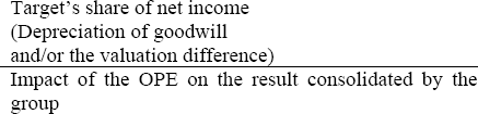
The EPS relution/dilution rate is given by the formula:
It is possible, as in the case of the takeover bid, to determine the accretive or dilutive nature of the operation before taking into account the depreciation of goodwill and/or the valuation difference. The OPE of A on B is accretive if the EPS of A after OPE is greater than the EPS of A before OPE, so:
where:
- – NRA: net result of the initiating company A;
- – RNB: net result of the target company B;
- – nA: number of shares in the capital of A before OPE;
- – nB: number of shares in the capital of B before OPE;
- – PA: price of A;
- – PB: price of B.
Finally, the takeover bid is accretive before taking into account the provisions for goodwill depreciation and/or the valuation difference if the P/E of the initiator is greater than the P/E of the target company. In the case of a direct merger, the operation is based on exchange parity and results in an increase in the capital of the acquiring company. However, such a transaction does not generate goodwill. Also, the impact of the operation on the net income group share of the acquiring company, which determines its rate of increase in EPS, is limited to the share of the net income of the absorbed company, which is apprehended following the merger-absorption. Hansen (1985) points out that takeover by way of a public exchange offer allows the shareholders of the target company to benefit from a part of the gains anticipated by the initiator of the operation.
The synergies correspond to the pre-tax surplus earnings that the companies that merge together could not have achieved in isolation. The first category of synergies relates to the costs linked to getting rid of the head office of one of the two companies, along with workforce reductions and improving supply conditions. The second category concerns development synergies, i.e. obtaining of new commercial outlets for the complementary products of the companies that come together. When examining merger events, Mandelker (1974) finds that the value created through synergies benefits the shareholders of the acquired company. This conclusion results from abnormal returns on the shares of the acquired companies, while the shares of the companies initiating the mergers show no significant gain or loss of return. Therefore, synergies represent the externalization of a gain that the shareholders of the acquired company realize only on the day of the merger. However, this potential should be detected and properly valued before the merger takes place in an efficient market. Ellert (1976) explains this by asserting that the management of acquired firms is inefficient, and that mergers turn out to be the best way to allow the market to play its role in optimizing the allocation of firm resources.
The debt ratio or gearing ratio – which corresponds to the ratio between consolidated net financial debt and consolidated shareholders’ equity – is also a criterion for investment decisions. A debt ratio greater than 1 is deemed unacceptable and results in a downgrade of the company’s financial rating by specialist agencies (Moody’s, Standard & Poor’s, Fitch IBCA, etc.), as well as an increase in the cost of the debt. This situation therefore implies a strategic refocusing of the group leading it to pursue a divestment policy, with the aim of restoring its financial structure. The takeover bid leads to an increase in net financial debt due to the debt generated by the operation. Equity increases by the amount of minority interests (those shown on the target’s balance sheet and those generated by the operation). They then correspond to the share of the net equity of the target that is not held by the initiator at the end of the takeover operation, given an offer’s success rate of less than 100%. The OPE does not generate increased debt to finance the operation. Equity, for its part, appreciates up to the minority interests that appear on the target’s balance sheet and due to the capital increase, including premium, that is generated by the operation. In the event of a direct merger, the impact on the debt ratio is almost identical to that of a public exchange offer:
- – increase in the net financial debt of the acquiring company by the amount of net debt of the absorbed company, if the latter is not fully consolidated before the merger-absorption;
- – increase in shareholders’ equity by recovering minority interests in the absorbed company (if the latter is not fully consolidated before the operation) and by the capital increase, including premium, generated by the operation.
- – Two ratios are considered by banks and analysts to be significant of the debt repayment capacity:
- – the ratio between the consolidated net financial debt and the consolidated self-financing capacity (SFC)34 must be less than 3;
- – the ratio between the consolidated net financial debt and the consolidated EBIDTA must be less than 4.
The takeover bid, financed by an increase in net financial debt, results in a reduction in financial income and a change in corporation tax due to the tax deductibility of interest charges. In addition, if the initiator does not consolidate the target before the full consolidation transaction, its consolidated cash flow and consolidated EBITDA are, respectively, increased by those of the target. The OPE does not generate additional financial costs. Consequently, the consolidated CAF and EBITDA are only increased by those of the target, if the latter is not fully consolidated before the operation. The impacts of the direct merger on CAF and EBITDA are identical to those of a takeover bid: respective recovery of the CAF of the absorbed company and its EBITDA insofar as the latter is not fully consolidated before the merger-absorption.
The financial expense coverage ratio, which must be greater than 4, is the ratio between consolidated feedback and consolidated financial expense net of financial income. If the target company is not fully consolidated before the offer (or the merger), the operating profit and the net financial expenses of the initiating company increase, respectively, from those of the target at the end of the transaction. In the case of a takeover bid, the financial expenses increase by the amount of the acquisition debt.
Following a takeover bid, the company that contributed the shares of the target company it held to the offer will show exceptional income in its consolidated accounts. This result relates to the difference between their sale price and their cost price on the consolidated balance sheet. The latter corresponds to the share of equity held by the transferor and possibly revalued after the acquisition of securities. In addition, the goodwill disappears from the transferor’s balance sheet through a depreciation item, insofar as its value corresponds to the estimate of future profits that the transferred company was expected to provide to the transferor. Finally, the potential payment of tax on the capital gain within the sale by the transferor reduces its consolidated income (group share) by the same amount. In total, the impact of a sale on the consolidated income of a group corresponds to:

At the end of a takeover bid, the transferor renounces their share in the future results of the target company. However, they save financial charges on their acquisition debt, which they can repay. In addition, they may place an amount of their capital gain on sale on the market. Considering that the placement rate and the borrowing rate are close, the sale results in a loss of a share of net income and in a loss of financial income, calculated on the basis of the sale amount.
1.4.2.3. Share buybacks
The PSBO (public share buyback offer) may target any percentage of the capital provided that the company has a sufficient amount of distributable reserves35. The PSBO is a public offer under a simplified procedure. The company must justify the offer price in a note approved by the AMF through a multi-criteria analysis. The capital gain generated by shareholders who follow the offer is treated for tax purposes as a dividend, not giving rise to the right to tax credit.
The PSBP (personal share buyback program) gives rise to the publication of an information document not approved by the AMF. This document specifies:
- – the objectives of the program;
- – the legal framework of the operation (text of the draft resolution of the general assembly);
- – the terms of the operation:
- - percentage of the target capital capped at 10% after deduction of shares already held by the company,
- - duration and timing of the operation. The period is capped at 18 months from the date of the general meeting called to rule on the operation,
- - financing of the operation corresponding to self-financing or debt;
- – elements that make it possible to assess the financial impact of the operation in terms of:
- - debt ratio: net financial debt is increased by the amount of the repurchase and shareholders’ equity is reduced by the same amount (when the repurchased securities will be canceled),
- - EPS before and after taking into account dilutive securities. The net result is reduced by financial expenses (net of IS) generated by the increase in net financial debt. The number of shares is reduced by the number of shares canceled at the end of the transaction;
- – the tax consequences of the operation:
- – for the company initiating the transaction, there is no tax impact if the repurchased securities are subsequently canceled. If the securities are not intended to be canceled but sold or transferred at a price different from that of their repurchase, the operation will have an impact on taxable income,
- – for the transferor, the capital gain is taxed for individuals and companies if the securities are resold less than 2 years after their acquisition. If the securities sold within the framework of the buyback offer have been held for more than 2 years, only 5% of the capital gain is reintegrated into tax income for the share of costs and charges;
- – the intentions of the persons controlling the initiator alone or with others with regard to the sale of securities as part of the transaction;
- – recent significant events relating to the company since the last publication of its information (annual report, information note relating to a financial operation, etc.);
- – the person responsible for the information note, usually the CEO of the initiating company.
Therefore, if a company intends to buy back up to 10% of its capital, it chooses the method of the operation according to its “tax customers”:
- – if the shareholders are mainly individuals, the PRAP is chosen;
- – if the shareholders are companies that are eligible for the “parent-subsidiary” scheme, the OPRA is chosen;
- – if the shareholders are companies which have held the securities for more than 2 years (and their participation is insufficient to allow them to benefit from the “parent-subsidiary” scheme), the company will choose the PRAP.
In the context of an acquisition of a listed target by takeover or takeover bid, valuation by traditional approaches favor negotiations between buyer and seller. When a shareholder wishes to withdraw from the capital of a company, they undertake negotiations with another company through an advisory bank. The acquirer who takes control of the target and integrates it into their overall strategy must agree to pay a control premium36. The transferor can use investment funds that take control of the target company via a takeover holding company. The value of the target is then no longer to be assumed but is proven: it represents the maximum amount of funds that can be raised by the takeover holding company in the form of capital, subscribed by the investment and debt fund(s). Determining the value of the target company means structuring how the holding company is financed.
An LBO (leverage buy out) is the purchase of a company financed by debt through a buyout fund that involves the managers of the company from a financial point of view. What is more, the goal of the buyout is not only to obtain an enhanced level of profitability by playing on the leverage effect, as no value is created. The buyout’s success is mainly explained through an increase in motivation of the leaders who are more invested in the success of the company. A better allocation of resources in favor of the shareholders will be achieved. The key interests of managers are therefore twofold: a financial interest relating to their immediate or potential participation (stock options) in the capital, and a desire to maintain their jobs and their reputation by ensuring that the company does not go bankrupt. Highly profitable and without much investment potential, mature companies are the perfect candidates for buyouts. Jensen (1989) demonstrates that in the absence of heavy debt, the natural temptation of managers is to use their significant free cash flow to increase their size, to the detriment of their profitability, by overinvesting or by diversifying out of their business verticals. This most often leads to the destruction of value. The only value creation enabled by debt lies in the significant demand it places on managers to better manage economic assets.
1.4.3. Leveraged buyout operations
A leveraged buyout operation or LBO consists of acquiring a target company by an ad hoc takeover holding company which is financed to a large extent by debt. The acquisition of the holding’s equity solely by investors results in a down payment that is less than that which would be necessary to purchase the target’s shares, thus taking full advantage of the leverage effect (financial profitability of the target company above the cost of the debt).
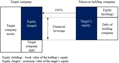
The holding’s acquisition debt is reimbursed by the dividends paid by the target and potentially by the cash provided by the exit from the LBO. This is the reason why the latter assumes certain conditions previously met to ensure the viability of the framework and to generate an acceptable level of risk. Also, the target must exercise their activity in a mature sector that requires moderate investments and holds low debt, in order to promote the distribution of high dividends to the takeover holding company. Environmental threats must be limited in order to reduce the risks that relate to the realization of the business plan in terms of competitive intensity, risk of calling into question the position of the target due to technological innovation and to cyclicality of activity.
The target company must also have a reliable and realistic business plan on which the financial simulations are based. It is important to have good visibility on the exit by IPO or by sale to an industry player or to another fund. We may frequently observe the transferor reinvesting in the capital of the takeover holding company. This reinvestment then secures the investment of the new fund, insofar as it constitutes a pledge to keep the current management in place, and gives credibility to the business plan relating to it. The conditions for a transferred reinvestment are the same as those of the emergence of the new fund. Reinvestment is also advantageous for the transferor because by carrying out such an operation, they are then about to mobilize only part of the cash received. In addition, they will benefit from the same IRR as the new fund as well as an upside potential when it exits the LBO, and thus will be able to benefit from certain tax advantages.
The target sale price is capped up to the maximum amount of funds likely to be raised by the buyout holding company. The amount of acquisition debt is directly linked to the expected profitability of the target company. The amount is calibrated according to several constraints. The first is to integrate a repayment over a period of 7–9 years, using the dividends distributed by the target to the holding company (assuming that the profit distribution rate of the target is at 100% from the start of the LBO). The second is to calibrate the operation so that the holding company retains slightly excess cash flow, so as not to generate additional financing needs. The third is to comply with certain financial ratios (covenants) which allow lending institutions and financiers to effectively control the smooth running of the LBO. Equity is set at a level that ensures that investors (and investment funds) receive an internal rate of return (IRR) of around 20–30% in 3 years, in the event of an exit from the fund by IPO or by transfer to a manufacturer or another fund on the basis of a multiple of gross operating surplus or operating profit. The target value is actually slightly less than the sum of the values of equity and of the debt of the holding company. Indeed, the latter must also finance various costs relating to the acquisition (of around 3–4% of the transaction value). These expenses generally correspond to the costs of hiring lawyers, getting advice, legal, accounting and tax audits and the payment of a commitment fee on the acquisition debt.
Optimizing the holding’s finances during the first years of the LBO will mean that part of the repayment of the acquisition debt is deferred. This senior debt is broken down into two parts. The first, called part A (80% of the total amount), is repayable by capital depreciation, and increases slightly over 7 years. The interest is calculated on the basis of the 6-month Euribor rate plus basis points. The second, called part B (20% of the total amount), is repayable at the end of 8 years and bears interest at the 6-month Euribor rate, also increasing from the basis point. The financing can be supplemented by a mezzanine debt, generally repayable after 9 years, or at 50% after 8 years and 50% after 9 years. Here, interest is calculated on the basis of the 6-month Euribor plus basis points to which the capitalized basis points are added. This mezzanine debt is accompanied by stock subscription warrants (SSW), which generate a capital gain that improves the performance of mezzanine financing providers (often referred to as “mezzaners”).
In the event that the holding’s cash flow is in deficit the first year, it is possible to envisage payment of an exceptional dividend by the target to the holding (with the condition of having distributable reserves), or the negotiation with banks of an “overfinancing” of the holding company, i.e. an increase in acquisition debt making it possible to cover cash requirements during the year. Kaplan (1989) and Smith (1990) show in particular that, over the period 1980–1985, the LBO improved the efficiency and performance of the acquired company.
The reduction in the tax payable by the group, made up of the holding company and the target, optimizes the operation thanks to tax integration. The tax group can use the tax deficit created by financial charges and the depreciation of acquisition costs of the holding company when the latter does not have taxable income (dividends go up tax-free within the scope of integration tax). The taxable results of the target are thus partially neutralized by the holding’s deficit for tax purposes. Thus, the target pays the holding company the corporate tax (IS) that it would have paid to the public treasury, in the absence of fiscal integration. The tax is liquidated vis-à-vis the holding company according to the principle of installments. In other words, during year N, down payments on corporate tax are paid for the current year and the liquidation balance37 is adjusted during the following year. In addition, the holding company pays the tax, the base of which corresponds to the taxable result of the target, reduced by the holding’s tax deficit. The conditions for reinvesting target shareholders in the capital of the takeover holding company can be optimized. The first axis concerns the contribution of part of the shares of the target to the takeover holding company. In this case, the capital gain on the disposal generated by the contributor is tax deferred until the date of disposal of the securities of the holding company which paid for the contribution. The second axis concerns the transfer of securities within the tax consolidation scope of the transferor. In this case, the takeover holding company must be part of the tax consolidation scope of the transferor before the LBO, and the entry of equity investors must be temporarily limited to less than 5%. This then assumes that 95% of the fund’s investment lies in the acquisition of bonds convertible into shares, or bonds redeemable into shares. Thus, the capital gain is unrealized. The third axis is around the reinvestment of the transferor as a physical person, in the amount of more than 25% of the capital of the holding company. In this case, the reinvestment amount is deductible from the ISF, and the shares held are assimilated to a work tool.
Distributing all of the target’s income to the holding company (achieved during the previous financial year) leads to recalculating the financial debt and the target’s financial income. Beyond the business plan period, forecasts can be extended over 9 years using the following assumptions:
– activity growth rate equal to that expected for the last year of the business plan, or linear convergence (linear interpolation) towards a more normative activity growth rate (somewhere between 2 and 3%);
– main ratios observed in the last year of the business plan maintained beyond:
- - EBIDTA or EBIT margin rate,
- - ratio: depreciation expense/turnover,
- - ratio: investments/revenue. The level of investments must, however, be in relation to the observed growth if this is variable,
- - ratio: net working capital/revenue.
In the absence of additional information, minority interests and the projections for risks and charges in the opening balance sheet are assumed to be constant over the entire period selected for the LBO. The construction of the target’s balance sheet is based on forecasted cash flows which make it possible to determine the net financial debt.

The balance sheet at 31/12/N is obtained from that at 31/12/N-1:
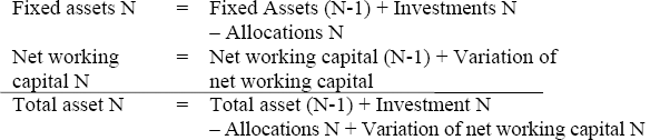

This presentation makes it possible to demonstrate, by recurrence, the balance sheet balance at 12/31/N, under the assumption of a balance sheet balanced at 12/31/N-1, by replacing cash flow by its value:
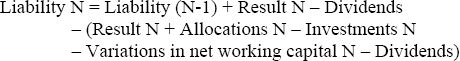
By simplifying by result N and Dividends N and by considering the fact that the liability (N-1) is equal to the asset (N-1), we therefore have:

In addition, the maximum debt of the holding company must be set at a level such that the cash flow always remains positive. The net result of the holding company on which the determination of its cash flow is based supposes the preliminary calculation of the tax due, under the tax consolidation agreement. The tax paid by the integrated tax group is determined on the basis of the taxable result of the target, assimilated to its current result before taxes (CRBT) from which the depreciation and amortization of acquisition costs are deducted, on the one hand, and, on the other hand, the financial expenses on the acquisition debt, to which the financial income generated by the investment of the takeover holding company are added where applicable.
And so:

The holding’s net income includes dividends received from the target, tax received from the target, depreciation and amortization of acquisition costs, financial costs generated by the acquisition debt and the balance of tax payable to the public treasury.
And so:
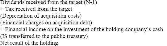
The holding company’s balance sheet is based on its cash flow, determined from net income and the repayment schedule of the acquisition debt. The cash flow of the holding company is determined from its net income. It is then necessary to reinstate the amortization of acquisition costs, and to deduct the amount to be repaid from the acquisition debt.
And so:
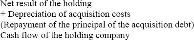
Senior acquisition debt is repaid by constant amortization or, in a more aggressive case, by progressive amortization.
The holding company balance sheet then shows the cash flow to be maintained at a positive level:
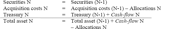
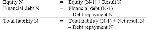
Replacing cash flow N by its value makes it possible to establish, by recurrence, like for the target, the balance of the holding company balance sheet.
The maximum amount of the holding’s equity must be set at a level such that the IRR of equity investors reaches the desired level (around 30% in 3 years).
It is determined by successive iterations by simulating different levels of debt. The IRR of equity investors is determined by comparing the valuation of the group (holding and target) at the time of their exit from the holding’s capital, with the valuation retained for the target at the time of their entry:
- – Vn: equity value of the set made up of the holding company and the target in n years; in other words, Vn is the exit value of equity investors (private equity funds);
- – V: amount of fund investment;
- – i: IRR required by the fund.
During the entire investment period, the fund does not receive dividends, so as to optimize the service of the acquisition debt. Therefore, we find:
V is the present value at the required IRR of the output value. The group’s Vn value (holding and target) that results from stock market comparisons (application of a multiple of EBIT or EBITDA) includes its net financial debt, from the consolidated balance sheet.
Table 1.12. Consolidated opening and closing balance sheets of the holding company
| Consolidated opening balance sheet at 31/12/N | Consolidated closing balance sheet at 31/12/N+1 |
| Target fixed assets N Target working capital N Holding costs N Goodwill N |
Target fixed assets N+1 Target working capital N+1 Holding costs N+1 Goodwill N |
| Total consolidated asset N | Total consolidated asset N+1 |
| Holding equity N Consolidated reserves N Target net debt N Holding net debt N |
Holding equity N+1 Consolidated reserves N + target result N+1 Target net debt N+1 Holding net debt N+1 |
| Total consolidated liability N | Total consolidated liability N+1 |
By way of illustration, an LBO was carried out on the Carrefour SA company. Based on the forecasts from zonebourse.com analysts, the income statement is extended according to the same logic as that which underlies the valuation by the DCF method:
- – linear convergence of the activity growth rate from 5.4% in 2016 (last year of financial analyst forecasts) to 3% in 2021;
- – maintenance from 2016 of the following ratios observed:
- - operational margin of 5.4%,
- - ratio reporting depreciation and amortization to turnover at 1.9%;
- – cost of debt at 3.5% from 2017;
- – IS rate at 38%.
The change in net financial debt from the last published balance sheet (2013) is based on forecast cash flows. These include:
- – dividends as part of a distribution rate of 100% in order to optimize the service of the holding company’s acquisition debt;
- – investments which converge linearly between 2017 and 2021 towards the amount of depreciation allowances for the last year;
- – the change in WCR determined from the WCR/turnover ratio (-7.7%) assumed to be constant within the business plan.
Table 1.13. Forecast of activity and operational profitability of the Carrefour SA
| Carrefour target income statement (€ million) | Production | Source zonebourse.com | Extension | ||||||
| 2013 | 2014 | 2015 | 2016 | 2017 | 2018 | 2019 | 2020 | 2021 | |
| Turnover | 74,888 | 75,384 | 78,760 | 81,672 | 84,578 | 87,469 | 90,337 | 93,173 | 95,968 |
| Growth rate | 0.7% | 4.5% | 3.7% | 3.6% | 3.4% | 3.3% | 3.1% | 3.0% | |
| EBITDA | 3,669 | 3,840 | 4,125 | 4,421 | 4,578 | 4,735 | 4,890 | 5,044 | 5,195 |
| EBITDA margin rate | 4.9% | 5.1% | 5.2% | 5.4% | 5.4% | 5.4% | 5.4% | 5.4% | 5.4% |
| (Allocations) | (1,432) | (1,413) | (1,511) | (1,572) | (1,628) | (1,684) | (1,739) | (1,793) | (1,847) |
| Allocations/turnover | -1.9% | -1.9% | -1.9% | -1.9% | -1.9% | -1.9% | -1.9% | -1.9% | -1.9% |
| EBIT | 2,237 | 2,427 | 2,614 | 2,849 | 2,950 | 3,051 | 3,151 | 3,250 | 3,348 |
| (Net financial costs) | (578) | (521) | (541) | (515) | (203) | (210) | (215) | (214) | (207) |
| Cost of debt | 3.5% | 3.5% | 3.5% | 3.5% | 3.5% | ||||
| RIBT | 1,659 | 1,906 | 2,073 | 2,334 | 2,747 | 2,841 | 2,936 | 3,036 | 3,140 |
| (IS) | (631) | (724) | (788) | (887) | (1,044) | (1,079) | (1,116) | (1,154) | (1,193) |
| IS rate | 38.0% | 38.0% | 38.0% | 38.0% | 38.0% | 38.0% | 38.0% | 38.0% | |
| Net result | 1,028 | 1,182 | 1,285 | 1,447 | 1,703 | 1,761 | 1,820 | 1,882 | 1,947 |
| Cash flow of target Carrefour (millions €) | Production | Prolongation | |||||||
| 2013 | 2014 | 2015 | 2016 | 2017 | 2018 | 2019 | 2020 | 2021 | |
| Net income | 1,028 | 1,182 | 1,285 | 1,447 | 1,703 | 1,761 | 1,820 | 1,882 | 1,947 |
| (Dividend) | (1,028) | (1,182) | (1,285) | (1,447) | (1,703) | (1,761) | (1,820) | (1,882) | |
| Depreciations & Amortizations | 1,413 | 1,511 | 1,572 | 1,628 | 1,684 | 1,739 | 1,793 | 1,847 | |
| (Investments) | (2,311) | (2,302) | (2,416) | (2,302) | (2,188) | (2,075) | (1,961) | (1,847) | |
| (AWCR) | 38 | 260 | 225 | 224 | 223 | 221 | 219 | 216 | |
| Cash flow = Net debt | (706) | (427) | (458) | (194) | (224) | (56) | 113 | 280 | |
Table 1.15. Provisional assessment of the Carrefour SA target
| Simplified financial statement of the target Carrefour (millions €) | Production | Extension | |||||||
| 2013 | 2014 | 2015 | 2016 | 2017 | 2018 | 2019 | 2020 | 2021 | |
| Assets | 22,107 | 23,005 | 23,796 | 24,640 | 25,314 | 25,819 | 26,155 | 26,323 | 26,323 |
| WCR | (5,775) | (5,813) | (6,074) | (6,298) | (6,522) | (6,745) | (6,966) | (7,185) | (7,401) |
| Total asset | 16,332 | 17,192 | 17,722 | 18,342 | 18,792 | 19,074 | 19,189 | 19,138 | 18,922 |
| Equity | 8,597 | 8,751 | 8,854 | 9,016 | 9,272 | 9,330 | 9,389 | 9,451 | 9,516 |
| Provisions | 3,618 | 3,618 | 3,618 | 3,618 | 3,618 | 3,618 | 3,618 | 3,618 | 3,618 |
| Net debt | 4,117 | 4,823 | 5,250 | 5,708 | 5,902 | 6,126 | 6,182 | 6,068 | 5,788 |
| Equity & liabilities | 16,332 | 17,192 | 17,722 | 18,342 | 18,792 | 19,074 | 19,189 | 19,138 | 18,922 |
| WCR/CA | -7.7 % | -7.7 % | -7.7 % | -7.7 % | -7.7 % | -7.7 % | -7.7 % | -7.7 % | -7.7 % |
| Holding’s debt due date (millions €) | Production | Extension | |||||||
| 2013 | 2014 | 2015 | 2016 | 2017 | 2018 | 2019 | 2020 | 2021 | |
| Amount left to pay | 6,900 | 6,038 | 5,175 | 4,313 | 3,450 | 2,588 | 1,725 | 863 | 0 |
| (Amortization of principal) | (863) | (863) | (863) | (863) | (863) | (863) | (863) | (863) | |
| In % of nominal | 12.50% | 12.50% | 12.50% | 12.50% | 12.50% | 12.50% | 12.50% | 12.50% | |
| Euribor 6 M | 0.18% | 0.18% | 0.18% | 0.18% | 0.18% | 0.18% | 0.18% | 0.18% | |
| Margin on Euribor (spread) | 2.75% | 2.75% | 2.75% | 2.75% | 2.75% | 2.75% | 2.75% | 2.75% | |
| Cost of SWAP | 1.00% | 1.00% | 1.00% | 1.00% | 1.00% | 1.00% | 1.00% | 1.00% | |
| Cost of debt | 3.93% | 3.93% | 3.93% | 3.93% | 3.93% | 3.93% | 3.93% | 3.93% | |
| Average debt | 6,469 | 5,606 | 4,744 | 3,881 | 3,019 | 2,156 | 1,294 | 431 | |
| Financial costs | 254 | 220 | 186 | 153 | 119 | 85 | 51 | 17 | |
Table 1.17. Provisional accounts of the holding company of the Carrefour SA target
| Holding’s income statement (millions €) | Production | Prolongation | |||||||
| 2013 | 2014 | 2015 | 2016 | 2017 | 2018 | 2019 | 2020 | 2021 | |
| Dividends received from the target | 1,028 | 1,182 | 1,285 | 1,447 | 1,703 | 1,761 | 1,820 | 1,882 | |
| (Financial costs) | (254) | (220) | (186) | (153) | (119) | (85) | (51) | (17) | |
| Tax received from the target | 724 | 788 | 887 | 1,044 | 1,079 | 1,116 | 1,154 | 1,193 | |
| (Tax to pay to the public treasury) | (628) | (704) | (816) | (986) | (1,034) | (1,083) | (1,134) | (1,187) | |
| Net income | 870 | 1,045 | 1,170 | 1,353 | 1,630 | 1,709 | 1,789 | 1,872 | |
| Tax group | Production | Prolongation | |||||||
| 2013 | 2014 | 2015 | 2016 | 2017 | 2018 | 2019 | 2020 | 2021 | |
| Target’s income before tax | 1,906 | 2,073 | 2,334 | 2,747 | 2,841 | 2,936 | 3,036 | 3,140 | |
| (Financial costs of H) | (254) | (220) | (186) | (153) | (119) | (85) | (51) | (17) | |
| Income of tax group | 1,652 | 1,853 | 2,148 | 2,595 | 2,722 | 2,851 | 2,985 | 3,123 | |
| (Tax to pay to the public treasury) | (628) | (704) | (816) | (986) | (1,034) | (1,083) | (1,134) | (1,187) | |
| Holding’s cash flows (millions €) | Production | Prolongation | |||||||
| 2013 | 2014 | 2015 | 2016 | 2017 | 2018 | 2019 | 2020 | 2021 | |
| Net income | 870 | 1,045 | 1,170 | 1,353 | 1,630 | 1,709 | 1,789 | 1,872 | |
| (Amortization of the principal) | (863) | (863) | (863) | (863) | (863) | (863) | (863) | (863) | |
| Cash flow = D Treasury | 8 | 183 | 307 | 490 | 767 | 846 | 926 | 1,009 | |
| Balance sheet of the holding | Production | Prolongation | |||||||
| 2013 | 2014 | 2015 | 2016 | 2017 | 2018 | 2019 | 2020 | 2021 | |
| Shares of the target | 16,641 | 16,641 | 16,641 | 16,641 | 16,641 | 16,641 | 16,641 | 16,641 | 16,641 |
| Treasury | 0 | 8 | 191 | 498 | 988 | 1,755 | 2,601 | 3,527 | 4,537 |
| Total asset | 16,641 | 16,648 | 16,831 | 17,138 | 17,628 | 18,395 | 19,242 | 20,168 | 21,177 |
| Equity | 9,741 | 10,611 | 11,656 | 12,826 | 14,178 | 15,808 | 17,517 | 19,305 | 21,177 |
| Acquisition debt | 6,900 | 6,038 | 5,175 | 4,313 | 3,450 | 2,588 | 1,725 | 863 | 0 |
| Equity & liabilities | 16,641 | 16,648 | 16,831 | 17,138 | 17,628 | 18,395 | 19,242 | 20,168 | 21,177 |
Determining the acquisition debt falls within the following framework:
– linear amortization over 8 years;
– cost of debt from the 6-month Euribor which includes a hedging cost (1%) and a margin (2.75%);
– amount set in such a way that the holding company cash flow is always positive.
The amount of the holding’s equity (€9.7 billion) is determined so that the 3-year internal rate of return (IRR) for investors (private equity funds) is 20% (Table 1.18).
Table 1.18. Determination of the capital amount of the takeover holding company
| Determination of the holding’s capital | Production | Prolongation | ||
| 2013 | 2014 | 2015 | 2016 | |
| Market capitalization of the target | 16,576 | |||
| Net debt | 4,117 | |||
| Entreprise value | 20,693 | |||
| EBIT | 2,237 | |||
| Multiple of Ebit | 9.3 | 9.3 | ||
| EBIT | 2,849 | |||
| Enterprise exit value | 26,354 | |||
| Net debt of the target | 5,708 | |||
| Acquisition debt of H (rest to pay) | 4,313 | |||
| (H treasury) | (498) | |||
| Consolidated net debt exit from target | 9,523 | |||
| Economic value of exit equity | 16,832 | |||
| IRR required by the investment fund | 20% | |||
| Entry capital of the takeover holding company | 9,741 | |||
Consequently, in the event of an LBO, Carrefour SA would be valued at €16.8 billion, or 1.5% more than its market capitalization.
1.5. Conclusion
The market value of economic assets is divided between the economic value of equity and net debt. According to the theory of equilibrium markets, there exists an optimal financial structure that would be linked to the tax savings due to the tax deductibility of interest charges. However, taking into account personal taxes, bankruptcy and restructuring costs call into question the validity of this reasoning, as it goes against the tax advantage of debt at the corporate level. Indeed, the value of an indebted business can be greater than that of a non-indebted business. The optimal debt ratio would be achieved when the present value of the tax savings, which results from additional debt, is simply offset by the increase in the present value of the costs of dysfunction and bankruptcy that this entails38. Moreover, integrating investor taxation turns out to be another constraint on this reasoning. Indeed, in practice, income from equity is taxed less than the income from debt, insofar as the tax advantage of debt for a company is lessened by the tax advantage of equity. In addition, in recent years, state tax reforms have tended to eliminate the corporate debt tax advantage39. Moreover, the theory of equilibrium markets considers the company to be a single actor. However, in practice, theories coming from organizations seem to reflect reality to a higher degree. Indeed, the decision to take out debt for a company is above all the result of agency conflicts between the various stakeholders of the company or of a desire to send a signal to the market that it is only a study of the structure and the cost (within the limit of debt ratios). Valuation methods estimate enterprise value in order to derive the economic value of equity. The three traditional methods based on wealth, stock market considerations and business plans are supposed to be combined to find the most accurate value. This exercise is particularly useful in the corporate control market. It helps guide the shareholders and orient the strategy to be implemented.
Depending on the contexts of specific financial structures, or on the company’s position in its life cycle, the literature on traditional valuation methods advocates for the use of some methods over others. These recommendations are derived from empirical results for which the authors first make theoretical adjustments. This means optimizing and making the application of these results more reliable in order to reach a fair value.
- 1 Enterprise value is equal to the economic value of equity and net debt. However, as long as the company is in a normal situation, the value of debts will fluctuate mainly according to the level of interest rates.
- 2 This rule can be applied sooner or later to companies that are not listed upon sale, merger, succession or increase in capital.
- 3 Market capitalization represents the economic value of equity and net debt, which represent a decreased value of loans granted by creditors for cash investments.
- 4 We may also call this “operational asset” or “capital employed”.
- 5 In practice, from the same sector of activity.
- 6 The threat of a Public Acquisition Offer is seen as a mode of external control.
- 7 If the share is made up of m categories of shares where nk represents the number of shares by k and pk, the category’s share price k, then the market capitalization equals
 .
. - 8 Some companies do not have them, while others that belong to the same sector of activity have recorded significant sums which could, therefore, bias the results.
- 9 The amount of commitment recognized increases each year to the extent that it is an updated amount.
- 10 This equation is systematically applicable even when different share categories are at play.
- 11 It is also possible to keep this enterprise value in order to realize the multiples of the previous year.
- 12 The amounts on the balance sheet and income statement aggregates from Shell’s 2013 registration documents are expressed in dollars. Therefore, the conversion made in Table 1.2 only relates to the final share price since the share listed on the Amsterdam Stock Exchange is expressed in euros.
- 16 Generally, g ∊ [0;4%] and k ∊ [8;15%]. In other terms, for the model to work properly, it is essential for the rate of return expected by shareholders is greater than the rate of growth of dividends.
- 17 FCF = EBIT – IS on the basis of EBIT + depreciations – Δ WCR – investments.
- 18 See the Appendix.
- 19 Source: banque-france.fr, website of Banque de France.
- 20 Source: zonebourse.com and fr.investing.com.
- 21 Source: zonebourse.com and fr.investing.com for betas and market capitalizations; reference documents for companies for net debt.
- 22 The request identifies information on the proposed financing, the history of the company, its current activity and its plan for future development (document the main parts of which are distributed to investors in the form of a prospectus).
- 23 Via the website: http://bear.cba.ufl.edu/ritter.
- 24 These are category A domestically traded shares.
- 25 http://www.amf-france.org.
- 26 The precedent condition may be linked to obtaining securities (expressed as a percentage of the capital or voting rights), at the end of the transaction. Furthermore, if the same initiator files various draft offers on separate companies, there may be an obligation to obtain a threshold for holding capital or voting rights on some or all of the target companies. Under merger control, if the proposed public offer is the subject of a notification to the European Commission, the Minister of the Economy or the competent authority of a Member State of the European Union or the United States, it is necessary to obtain the decision provided for in Article 6-1 (a) or (b) of Regulation (CEE) no. 4064/89, the authorization provided for in Article L. 430-5 of the French Commercial Code or any similar authorization issued by the institution in question.
- 27 This suspension may also affect other securities affected by the proposed offer.
- 28 The time limit begins to run again upon receipt of the required elements.
- 29 Articles L.233-10, L.225-207 and L.225-209 from the Trade Code.
- 30 Article L.233-10 of the Commercial Code (article 356-1-3 of law no. 66-537 from July 24, 1966).
- 31 Unless one or several of them already have this control and remain predominant and, in this case, as long as the balance of the respective holdings is not significantly changed.
- 32 Article L.233-10 of the Commercial Code (article 356-1-3 of law no. 66-537 from July 24, 1966).
- 33 Article L.225-209 of the Commercial Code.
- 34 The SFC corresponds to the difference between the products that are cashable/collected and the disbursable/disbursed charges. It can be calculated using net income by neutralizing accounting aggregates that impacted the net income without having an impact on cash flow (depreciation, amortization and provisions, book value of assets sold in terms of non- disbursable charges and reversals of depreciation and provisions, share of subsidies transferred to the income statement in terms of non-cashable income).
- 35 All reserves are distributable with the exception of the legal reserve and revaluation reserve.
- 36 If the target’s attractiveness is strong and/or if the competition with other prospective buyers is significant, they may agree to pay part of the valuation of the anticipated synergies.
- 37 Difference between IS actually due and the sum of installments already paid.
- 38 As the debt increases, the enterprise value is negatively impacted as the indebted company can no longer make a profit and therefore take advantage of the tax benefit. If the situation persists, the company finds itself in a difficult situation and is forced to incur bankruptcy costs (severance payments, legal costs). In addition, an indebted company must incur restructuring costs to meet its debt repayment deadlines and may lose profitable investment opportunities because it can no longer finance itself. These dysfunction costs correspond to reductions in research and development or training costs.
- 39 In France, since 2014, only 75% of interest is tax deductible.