
2
The Performance of the Assessment and the Creation of Value from Control Operations
2.1. Introduction
Theoretical adjustments aim first of all to reconcile the traditional view of the optimal financial structure with the Modigliani-Miller theorem. To do this, Farrar and Selwyn (1967), Brennan (1970) and Dickinson and Kyuno (1977) find that the integration of the taxation of individuals and their aversion to risk are key factors in determining the choice of additional debt for the company. Then, due to the simplicity of its implementation, the capital cash flow method of Ruback (1998) can prove to be an alternative approach to the DCF method without needing to change the valuation result. In addition, the concept of duration discussed by Arnold and North (2008) may be important to make the hypothetical parameters reliable when building a business plan through the DCF method. Finally, Shaffer (2006) attempts to integrate the risk of bankruptcy into the DCF method.
While from a theoretical standpoint, the discounted cash flow method seems to be the most reliable insofar as it takes into account a potential change in discounted cash flows at a rate that corresponds to the cost of capital, empirically, the preference of one valuation method over another depends on a variety of factors. In reality, according to Kaplan and Ruback (1995), if we are talking about leveraged buyout operations, the methods that adopt business plans actually prove to be more suitable than the approaches based on multiples. However, Alford (1992) asserts that the P/E ratio is more precise once an appropriate benchmark has been established. The sample should ideally include companies in the same industry with similar financial structures and portfolio value of assets. In the same way, according to Damodaran (2009), the valuation of a young company (whose cash flow forecasting is more than delicate, or at least, it must be carried out in the short term) seems to be able to be carried out from sales or net income, discounted at a target rate of return. Moreover, by focusing on specific contexts such as the takeover of companies that have gone bankrupt, Hotchkiss and Mooradian (1998) find that the prices paid are initially based on a valuation that results from the multiple of turnover or assets. However, given the large disparities between the prices paid and the initial valuations that emerge within such contexts, it seems that company valuation that relates to the negotiation margin of the different stakeholders is, in this context, more of an exercise used for strategic purposes than a purely financial tool aimed at uncovering real value. According to Gilson et al. (2000), these disparities are not the result of calculation errors but rather resulting from deficiencies in the quality of information and conflicts between agencies.
The valuation of a company is used in particular to estimate the value of its buyout so that the synergies that result from the transaction can create value. It therefore seems interesting to know whether empirically such situations prove to be true. When buying out companies that are bankrupt, Hotchkiss and Mooradian (1998) estimate that only the target company sees its share price increase in the days that follow the transaction. More generally, the study by Moeller et al. (2004) concludes that taking control of a company does not create value. Thus, the interest in conducting such operations is more linked to the reasons for expanding the group’s influence on the market, and is justified in terms of remuneration beyond simple errors of assessment, which are consequences of the unfounded optimism from business leaders.
2.2. Theoretical adjustments
In order to reconcile the traditional view of optimizing financial structures with the Modigliani-Miller theorem, Dickinson and Kyuno (1977) constitute a model in which they incorporate the tax on capital gains, dividends and interest earned. They believe that investors arbitrate their decision to participate according to the possible benefit of personal leverage. They note that if the market is dominated by aggressive investors who demonstrate significant risk aversion, the company would do well to go into debt. Conversely, if the market is dominated by cautious investors, additional debt would lessen the corporate tax advantage. Farrar and Selwyn (1967) assess corporate financial policies with respect to income after-tax that is received by an investor. Their study points to the affirmation that the policy of the financial structure depends on the marginal tax rates of investors and the policy of paying dividends. For his part, Brennan (1970) shows that the implementation of a leverage strategy that maximizes enterprise value turns out to be attractive to all investors, provided that the corporate tax rate is higher than the effective tax rate in the market.
Regarding the theoretical adjustments to the method of discounting cash flows, Ruback (1998) proposes a new approach: namely that of capital cash flows. It consists of finding the same result but by applying a simpler method that aims to make all of the cash available to investors (therefore including the tax advantages of interest charges). Arnold and North (2008) are more interested in making the DCF method more reliable. Based on the specific duration, they carry out a sensitivity study and calculate the effects of variations in the various parameters, which are initially subject to be critiqued as to their subjectivity. Finally, Shaffer (2006) adjusts the growth rate of the DCF method taking into account the risk of bankruptcy.
2.2.1. Reconciliation of the traditional view with the Modigliani–Miller theorem
Modigliani and Miller believe that the capital structure of a company does not have an impact on its value. Their model is essentially based on investor arbitration and their presupposed indifference to two opportunities that present the same risk and the same return. Including the effects of corporate taxes, they conclude that an increase in the level of debt increases the value of a business because of the tax deductibility of interest. Unlike their model, the traditional view is to determine an optimal level of debt (in terms of its effect on valuation). Dickinson and Kyuno (1977) propose a reconciliation between the traditional vision and that of Modigliani and Miller in the presence of taxation. Their objective is to demonstrate that an increase in the proportion of debt leads to a decrease in the average cost of capital (debt being a cheaper source of financing than equity) and, consequently, an increase in the value of company. Beyond a certain level of debt, the requirement for the company to make a profit implies an increased level of risk for holders of capital and for holders of debt. The latter therefore require a greater return on investment, which results in an increase in the average cost of capital. In addition, the taxation of individuals must be taken into account because they decide whether or not to invest, depending on the benefit they may derive from a potential leverage effect. In this context, Ferrar and Selwyn (1967) consider a tax rate based on the ownership interest in the company. Brennan (1970), on the other hand, takes into account trading opportunities in his study. Thus, the risk premium depends on the risk of the underlying security and the rate of dividends paid. The process of perfecting the optimization of the financial structure also applies to the DCF valuation method. Indeed, like Ruback (1998), it is possible to consider an alternative approach, that of capital cash flows (CCF), which seeks to preserve the very principle of discounting cash flows, while facilitating its implementation and by integrating the tax advantages which are linked to the deductibility of interest charges. In addition, Arnold and North (2008) prefer to focus on making the traditional DCF method more reliable by relying on the concept of duration. Through a sensitivity study, they determine the effects of variations in hypothetical parameters in order to measure the variation in cash flows.
2.2.1.1. A general framework
Dickinson and Kyuno (1977) assume that a company achieves result ![]() continuously (without risk of default, without taxation, which involves an arbitration process and the distribution of profits). Let us note:
continuously (without risk of default, without taxation, which involves an arbitration process and the distribution of profits). Let us note:
- – VU: market value of the deleveraged company U;
- – VL: market value of the indebted company L;
- – SL: market value of the company’s equity L;
- – BL: market value of debt L;
- – i: debt market interest rate;
- – kO: capitalization rate of capital income.
If an investor owns αVu of capital of the firm U, their return (excluding tax considerations) is ![]() . Consider the total return of an investment that consists of αSL parts equity and αBL parts debt. Equity – after deduction of financial interest – has the value
. Consider the total return of an investment that consists of αSL parts equity and αBL parts debt. Equity – after deduction of financial interest – has the value ![]() and debt αiBL.
and debt αiBL.
As the total return is also ![]() , the hypothesis about arbitration implies that the investments in U and L have the same value, i.e.:
, the hypothesis about arbitration implies that the investments in U and L have the same value, i.e.:
If the corporation tax is applied at rate t, the flow of net profit between corporation U and its investors is reduced to ![]() . On the other hand, if R corresponds to interest payments on the debt, the corresponding flow for firm L is
. On the other hand, if R corresponds to interest payments on the debt, the corresponding flow for firm L is ![]() . The difference in value between the two companies is therefore obtained by capitalizing the tR tax “subsidy” by the appropriate rate, i:
. The difference in value between the two companies is therefore obtained by capitalizing the tR tax “subsidy” by the appropriate rate, i:
The equation can be compared with the traditional view, which includes a tax effect on non-corporate debt. This effect, y, remains positive up to a certain level, beyond which it decreases and becomes negative:
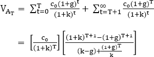
Dickinson and Kyuno include in their model the tax on capital gains g, on dividends d1 and on interest earned d2. They also assume that investors are indifferent to a dividend payout or retained earnings and that the value of the company does not depend on the level of reinvestment. Thus, they consider two deleveraged companies, U1 and U2, to be identical in all points except in terms of dividend policy. U1 preserves the tax saving ![]() within it, while U2 again carries
within it, while U2 again carries ![]() and distributes
and distributes ![]() of dividends. In the presence of capital gains and income taxes, the net gains between the two companies and the investors are, respectively:
of dividends. In the presence of capital gains and income taxes, the net gains between the two companies and the investors are, respectively:
By capitalizing these flows at the rate k1= k0(1 —t)(1 — d1) corresponding to the tax rate after capitalization:
The difference in value between the two deleveraged companies increases (decreases) and the retention rate b increases (decreases) provided that d1 > g (d1 < g)
Let us now consider two indebted companies L1 and L2, identical except in terms of dividend policy. The company L1, with the equity capital SL, distributes all the profits after tax in dividends, namely ![]() .
.
The company L2 again reports ![]() and distributes(1-b)
and distributes(1-b) ![]() .
.
The net gains between the two companies and the investors are:
and:
By capitalizing these two flows by the net return on equity e, and by income tax, we come to:
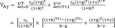
The value of L2 increases (decreases) and the retention rate b increases (decreases) provided that d1 > g (d1 < g). To introduce the effect of the dividend tax, d2, we must consider a deleveraged company U and an indebted company L. The net gain flow is:
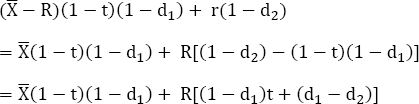
In the second term of the second equation of [2.19], we capitalize by using (1 – d2)i, i.e. the interest rate of the debt after tax, since this “tax subsidy” is effectively a certain flow. By combining the results of equations [2.18] and [2.19], we find the following equation, which incorporates all of the effects in the presence of taxation:
The increase in value from debt financing is only a function of t – as in the case of an individual investor – when d1 = d2. Indeed, the second term of equation [2.20] reduces tBL. However, due to the last term of equation [2.20], the value increases (decreases) and the retention rate increases (decreases) if d1 > g (d1 < g). It can also be noted that for the institutional investor, dividends are tax-deductible in order to avoid double taxation (d1 = 0 and d2 = g = t). Incorporating these values into equation [2.20] leads us to conclude that for such an investor, the tax advantage of “non-corporate” debt financing (which is negative) outweighs the tax advantage that comes from the company. Also, once the retention rate is increased (decreased), the value is decreased (increased). To summarize the results in a straightforward manner, we should assume that the retention rate b is constant for all companies with the same level of risk. The individual tax rate on the capital income, g’, is therefore the weighted average:
where:
The second term on the right-hand side of equation [2.26] is a measure of the “non-corporate” tax effect of debt financing. When d2 > g’, this term is negative and the corporate tax saving of debt financing is compensation. The taxation of individuals is therefore supposed to impact the financial policy of companies.
2.2.1.2. The impact of personal taxation on optimal financial policy
Dickinson and Kyonu (1977) believe that investors arbitrate their decision to participate according to the possible benefit of personal leverage. When considering the effects of the taxation of individuals on the financial policy of a company, Farrar and Selwyn (1967) focus, however, only on the net income received by an investor at a tax rate that depends on the share held in the company. Their use of this concept of net income as a criterion for best value overlooks the trading opportunities that are open in markets to an investor who does not adhere to a particular financial policy. Thus, Brennan (1970) extends the analysis of Modigliani and Miller by including personal taxation as a whole and observes impact on a company’s financial policy. Trading opportunities are taken into account, by applying the principle of market valuation, while the impact of alternative financial policies on the value of the company can be calculated.
2.2.1.2.1. Investor personal leverage and maximization of investor income after tax
According to Dickinson and Kyonu (1977), an investor who holds aSL of the capital of a firm L will receive a return of α(X – R)(1 – t)(1 – g’). By investing αVu in the capital of a firm U, a return of αX(1 –1)(1 – g’) is obtained. If the last investment is financed through a loan α(1 –1)(1 – g’)BL, which involves an interest of αR(1 – t)(1 – g’), its total return will be α(X – R)(1 – t)(1 – g’). This is exactly the return on the first investment, and we can therefore conclude that the amounts invested in both situations are identical:

And so:
Equation [2.27] should be compared to equation [2.31]. Both expressions give the effect of the personal tax, y, of debt financing with and without investor leverage. If the market is dominated by aggressive investors with significant risk aversion, equation [2.31] will be applied. Besides corporate tax, the advantage is to increase the level of debt. Conversely, if the market is dominated by more conservative investors, equation [2.27] will be favored and an increase in debt will wipe out the corporate tax advantage. In practice, it is impossible to define the direction and the magnitude of the personal tax effect, since it depends on investor preferences and the degree of taxation. Dickinson and Kyonu consider that the best effect should satisfy the following inequality:
Farrar and Selwyn (1967) assess corporate financial policies with respect to income after-tax that is received by an investor with a stake in a firm. And so it follows:
- – Y: net income flow (including capital gains) available to an investor who holds a share, net of any interest and taxes (personal or corporate);
- – X: operating profit per share of the company before payment of interest and taxes;
- – r: market interest rate;
- – Dc: amount of corporate debt per share;
- – Dp: amount of personal debt per share;
- – Te, Tp, Tg: Marginal tax rate on corporations, income and capital gains.
A first strategy consists of paying the profits in the form of dividends and taxing them through income tax. Thus, the net income per share of the investor is:
The costs after-tax to the investor of corporate and personal debt are:
The investor’s net income per share is reduced less by additional corporate debt than by additional personal debt, because of the additional corporate interest tax shield, which is offered by corporate tax. Thus, corporate debt is cheaper than personal debt for all investors, regardless of the marginal interest rate applied.
A second strategy is to convert the profit into capital gain and tax it at the investor’s level, at the capital gains tax rate. In this case, the net income available to the investor will be:
The costs of personal and corporate debt are:
From there, corporate debt is cheaper for the investor only if:
Equation [2.39] indicates that the relative effects of corporate and personal debt on the net earnings per share received by the investor depend on their marginal tax rates Tp and Tg. In general, investors with a low-tax bracket will find the impact of corporate debt on their net income relatively less favorable than those with a high-tax bracket. Thus, if the criterion for maximizing the net profit per share received by investors is accepted, we can conclude that it will always be optimal for a company to use residual profits to buy back shares rather than pay dividends, as long as the marginal tax rate on investors’ dividends exceeds that on capital gains. In addition, corporate debt will benefit investors in a company that pays dividends, although the value of the debt may directly depend on the marginal tax rate Tp of some investors. For a company that does not pay dividends, different financial policies may be optimal for different groups of investors, depending on their marginal tax rates. For example, investors with a marginal tax rate for whom Tp > Tc + Tg + TcTg will probably prefer the company to implement a “zero-debt” strategy, in order to maximize the amount of debt that investors can contract themselves, consistent with their desire for total debt per share. On the other hand, investors with a low marginal tax rate will seem to prefer the company to implement a “maximum debt” strategy. If such a strategy results in excessive leverage per share from an investor’s perspective, it can still be partially offset by their personal loans. However, in addition to coming across diverse opinions as to the optimality of the financial policy to be implemented (according to the group of investors to which one belongs), the criterion for maximizing the income after-tax paid to them implies that they have no choice: they remain shareholders and are therefore only interested in income per share. By adopting a more realistic assumption – i.e. thinking that investors have the ability to not only borrow and lend but also sell (or buy) their securities in the market – and assuming that opportunities are ultimately independent of decisions of a single firm, the welfare of investors can be maximized by optimizing the market value of the firm. Thus, the potential investor conflicts raised by Farrar and Selwyn are no longer relevant as long as the opportunities to “trade” in the market on the part of investors have been accepted. In other words, investors can perform their arbitration. As a result of this, the approach proposed by Farrar and Selwyn reveals itself to be too static, because it does not take into account the impact of issuing corporate debt on the net income Y of the investor, while neglecting the principle of company valuation.
2.2.1.2.2. Market valuation in a situation of uncertainty
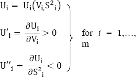
Analysis from Brennan (1970) builds on the generalized CAPM from Sharpe (1964), Lintner (1965) and Mossin (1966) by incorporating the effects of tax on income through dividends and on capital gains. We then assume that the utility functions Ui(i = 1,...,m) of investors depend on the mean Vi and the variance S2i of the returns after-tax from the portfolios:
Investors are supposed to trade n + 1 securities:
- – security 0 is supposed to have an initial value and a known terminal value q;
- – n remaining securities have an initial value pj (j = 1,..., n); an unknown terminal value πj;
- – each security j (j = 1,..., n) gives the right to a final dividend dj already known at the start of the period;
- – the terminal values of the securities have a covariance Sjk (j = 1,..., n);
- – each investor i (i = 1,..., m) has an initial allocation of X0ji securities j (j = 1,..., n), and, by trading with other investors, we arrive at a situation of equilibrium in the position of the assets at Xji(j = 1,..., n);
- – each investor has a marginal tax rate on tdi dividends and on tgi capital gains that are constant and independent of the choice of portfolio.
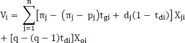
The expected return after-tax on the portfolio of investor i is:
And the various of return after-tax is:
And so, the investor maximizes their utility function:
This utility function is subject to the investor’s budget constraint:
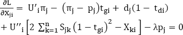
The first-order conditions of maximum constraints are obtained by using the Langrangian expression:
Any by setting its partial derivative to be equal to zero for Xji(j = 1,...,n) and λ gives:
When looking at [2.41], we note that:
And when looking at [2.42], we note that:
And so, we obtain these maximum constraints as conditions in addition to that of the budget (equation [2.47]):
By eliminating λ between [2.52] and [2.53] and through a process of simplification, we get:
where ![]() is proportional to the investor’s marginal rate of substitution between the expected return and the variance. Assuming that the second-order conditions for the maximum constraints are satisfied, equation [2.54] gives the equilibrium relation between the covariance of the return of the security j (j = 1,..., n) and the risk premium after expected tax by security j. The n equations of [2.54], which are correlated with the budget constraint equation [2.47], are sufficient to determine the equilibrium of the investor’s portfolio in the holding of their n + 1 securities. We may note that when wi enters as a constant in [2.54], the investor’s relative holdings n securities are independent of the exact model of their utility function but not of their marginal tax rate tdi and tgi. Market equilibrium is based first of all on the fact that each investor has a portfolio equilibrium, i.e. that equations [2.47] and [2.54] are verified for each of them (i = 1,..., m) and second that the securities market allows:
is proportional to the investor’s marginal rate of substitution between the expected return and the variance. Assuming that the second-order conditions for the maximum constraints are satisfied, equation [2.54] gives the equilibrium relation between the covariance of the return of the security j (j = 1,..., n) and the risk premium after expected tax by security j. The n equations of [2.54], which are correlated with the budget constraint equation [2.47], are sufficient to determine the equilibrium of the investor’s portfolio in the holding of their n + 1 securities. We may note that when wi enters as a constant in [2.54], the investor’s relative holdings n securities are independent of the exact model of their utility function but not of their marginal tax rate tdi and tgi. Market equilibrium is based first of all on the fact that each investor has a portfolio equilibrium, i.e. that equations [2.47] and [2.54] are verified for each of them (i = 1,..., m) and second that the securities market allows:
where X0j is the exceptional offer of security j. Then, by adding [2.54] on all the investors:
where:

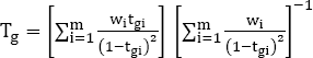
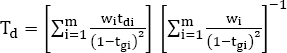
We note that Td and Tg are weighted averages of the tax rate on dividends and on investor capital gains, where the weights depend on the marginal rate of substitution of investors between the expected return and the variance of that return. Let us define new variables:
- – r = q – 1 the risk-free interest rate;
- –
 the eventual return of the dividend on security j (j = 1,..., n);
 - –
 the return on investment on security j (j = 1,..., n).
We note that:
where M is the total market value of securities and Qk (k = 1,..., n) and part of the security k in the total market value. Then, by dividing [2.56] by pj, and by transposing the terms and making the substitutions of returns:
where![]()
Finally, equation [2.62] can be simplified by noting that ![]() Rm, where Rm is the rate of return on the entire market portfolio:
Rm, where Rm is the rate of return on the entire market portfolio:
and [2.62] becomes:
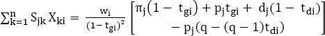
Equation [2.64] therefore expresses the basic principle of market valuation in a situation of uncertainty when investors have different tax rates, and it shows that the risk premium that is required or expected on security j (j = 1, ..., n) (Rj – r) is a function of the risk characteristics of the security COV(Rj,Rm) and its expected dividend rate δj. Intuitively, this result indicates that for a given level of risk, investors demand a higher total return on a security; the dividend rate must be higher since its tax rate is higher than that of capital gains.
2.2.1.3. Reconsidering the Modigliani-Miller theorem
2.2.1.3.1. The dividend payment constraint
Let us consider that there is no growth and that the future can be looked at as a series of identical periods where, in each of them, the market equilibrium condition of equation [2.64] is expected. In addition, at each period, the company receives a flow of operating income X, which is taxed at the IS rate τ. The company is supposed to pay a dividend D and buy back or issue shares at the end of each period while its market value V is constant. Assuming that investors’ risk taking and tax rates remain constant over time, expected future gains will be capitalized at a constant rate ρ. The possibility of a change in the value of the business due to a recapitalization of expected future earnings is excluded. Therefore, the end-of-period value of the company Vt, after dividends have been paid but before the shares have been redeemed or issued, will be equal to the value of the company at the start of the period, plus the result of operating net of tax minus dividends, namely:
Let us make R the rate of return of securities of the company:
and:
As a result, the value of company V can be written as the capitalized value of expected gains after tax:
where the rate of capitalization ρ is given by the condition of an equal [2.64]:

where ![]() will be the prospect of the dividend yield on the company’s securities. Then, by substituting ρ in [2.69] and adjusting it, we reach:
will be the prospect of the dividend yield on the company’s securities. Then, by substituting ρ in [2.69] and adjusting it, we reach:
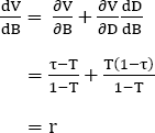
Equation [2.70] is a general valuation equation for the company that expresses its value as a function of the flow of net income from operations, and the amount of dividends paid in each period. To calculate the effect of alternative dividend policies on the value of the firm, we must partially differentiate [2.70] from D:
Equation [2.71] demonstrates that if the market value maximization criterion is accepted and if T> 0, investors have no interest in receiving dividends: share repurchases are preferred regardless of marginal tax rates. However, since most companies in fact pay regular dividends, such behavior needs to be streamlined, so that it is a real or a perceived constraint. Thus, it is necessary to presume that the company is subject to such a constraint.
Let us suppose that a company possesses an amount of bonds B whose interest rate is r. The market value of its capital is:
But E can also be considered as the net income expected by capital owners (X – rB)(1 – τ), capitalized at a rate of ρE depending on the risk and the composition of the capital income flow:
The constraint on the systematic share buyback can be written as such:
Equation [2.76] implies that the amount paid in dividends and the net interest payment are at least as large as the average flow of net income. We will note that:
Let us consider the effects of alternative debt levels on enterprise value under two constraints.
1) The constraint on the share buyback is not linked so that:
So, based on expression [2.75], we can deduce that:
And by looking at expression [2.80], we can deduce that:
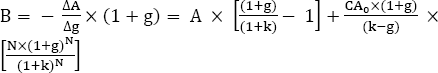
Equation [2.81] shows that a strong leverage strategy will maximize enterprise value and therefore be beneficial to all investors as long as the corporate tax rate τ exceeds the effective market tax rate T. However, the relative advantage of corporate debt is reduced by the existence of investor tax (T > 0).
2) The constraint on the repurchase of shares is linked so that:
So, the issuance of debt reduces the amount of dividends that must be paid by the interest cost of the net debt. Taking this into account:
And this is precisely the result obtained by Modigliani and Miller by neglecting the taxation of investors: if an amount of B bonds are issued, the value of the company is increased by τB. Thus, if the company is subject to a constraint on share buyback, Modigliani-Miller’s cost of capital proposals are unaffected by the existence of investor tax. This is based on the relationship between the amount of debt issued and the amount of dividends paid over the same period. The share buyback excludes the issuance of bonds, but there is a link between the debt issued and the dividends paid over the period that affects the valuation.
2.2.1.3.2. The effect of a debt issuance on enterprise value
Let V be the current value of the company and ∆B be the expected issuance of debt at the end of the first period. It is assumed that the company pays a constant dividend, does not incur other debt in subsequent periods and does not buy back shares. Thus, Vt is the enterprise value at the end of a period after debt has been issued and dividends paid.
We thus reach:
The total investor return throughout this period is:
The market balance makes it necessary for the expected value of equation [2.87] to be equal to:
where D1 is the amount of dividends paid in the first period. Then, by equaling [2.87] and [2.88] and by resolving V, we get:
The constraint on the share buyback for the first period can be written as:
Note that equation [2.90] explicitly excludes the use of the issue of bonds with a view to repurchasing shares.
Equation [2.91] shows that the total impact of expected debt issuance on enterprise value has two components: a direct impact ![]() and an indirect impact
and an indirect impact ![]() due to the consequent modifications of the dividends of the first period. If the redemption constraint of equation [2.90] is prohibited,
due to the consequent modifications of the dividends of the first period. If the redemption constraint of equation [2.90] is prohibited, ![]() and:
and:
Thus, when the repurchase constraint is prohibited, equation [2.92] shows that the issuance of debt will be advantageous if the IS rate τ is greater than T. However, when the repurchase of shares requires the issuance of bonds in order to pay dividends, the initial advantage of incorporating debt into the capital structure is diminished, because even though the enterprise value tends to increase by saving taxes (thanks to the bond issuance), the higher taxation of investors reduces this effect, to the extent that they have to pay the increase in dividends for the first period (brought about by the issuance of bonds).
After trying to refine Modigliani and Miller’s approach with regard to the financial structure and its impact on enterprise value, taking into account, in particular, the taxation of individuals, we may question if it is actually possible to optimize valuation methods by discounting cash flows (especially DCFs). In this way, the objective is to propose an alternative method or, at least, to make the assumed parameters of the DCF model more reliable. The DCF model is majorly criticized for its subjectivity, which, beyond that, can generate significant variations in calculations from one analyst to another in the quest for fair corporate value.
2.2.2. Optimizing the valuation methods
Ruback (1998) presents an alternative to the traditional DCF method for assessing risky cash flows and obtaining enterprise value. The capital cash flow method ultimately provides an enterprise value that is identical to that reached in the free cash flow method. It exists because of the simplicity of its implementation. It therefore lends itself more easily to the valuation of companies that have been subject to transactions with a high leverage effect, companies that have undergone restructuring or major financing projects or, finally, any other operation in which the capital structure has been largely affected, because the CCF method consists of including all the cash available to fund providers, therefore including the tax advantages linked to interest charges. These reduce taxable income. As a result, corporation tax decreases, resulting in an increase in cash flow after-tax. In other words, the capital cash flows are equivalent to the free cash flows to which we add the tax deductibility of interest charges. Because it is included in cash flows, the appropriate discount rate must then be a pre-tax rate to avoid double counting. It corresponds to the WACC before tax. Thus, unlike the DCF method, the various parameters of the capital cash flow method are not subject to adjustments, depending on the situation. Indeed, unlike an essential re-estimate of the WACC in the event of variations in the financial structure over time, the impact of these modifications in the CCF method is zero, insofar as the tax advantages of interest charges are included in the cash flows considered and that the risk-free rate of the assets is a fixed discount rate. Without proposing an alternative valuation method to that of DCF, Arnold and North (2008) seek to make this approach more reliable by carrying out a sensitivity study, based on the concept of duration, in order to calculate the effects of variations in the assumed parameters and to propose a measure of the variation in cash flows. Shaffer (2006), for his part, integrates the risk of bankruptcy through an adjusted growth rate.
2.2.2.1. Tax deductibility of interest charges and residual profits
In the DCF method, the tax deductibility of interest decreases the WACC, which, by definition, is after tax. Tax benefits related to interest charges are therefore excluded from free cash flows. Problems arise when the WACC is impacted by large variations in the capital structure. If the latter is simple, i.e. composed of classic bank debt and ordinary shares, the capital cash flows are equal to the flows available to shareholders, in addition to the interest paid to debt holders. Ruback (1998) thus takes up the idea, which was developed in his previous work (Ruback 1986), which dictates that the tax advantages of interest charges associated with risk-free cash flows are equivalent to the increase in cash flows generated by these same benefits, or a decrease in the discount rate, i.e. the risk-free rate after tax. The analysis thus presents similar results for risky cash flows: they can be obtained by using the CCF or DCF method, for which the tax benefits are added to the FCF in the discount rate. Although free and capital cash flows treat the tax deductibility of interest charges differently, the two methods are algebraically comparable.
To illustrate, let us determine the WACC before tax:
where:
- – k= rf+ßERP;
- – i = rf + ßDRP;
- – rf = risk-free rate;
- – RP = risk premium;
- – βE et ßD= equity and debt betas.
And so:
and:
Moreover, note the beta of the deleveraged asset:
And so:
Note that the discount rate does not depend on the financial structure and should not be recalculated according to its variations. This therefore means that,in the CCF method, debt-to-enterprise value and equity-to-enterprise value ratios do not need to be estimated. Therefore, this eliminates much of the complexity that we encounter when evaluating from the DCF method. Let us remember:
where:
Capital cash flow is the cash flow expected by all fundraisers that incorporate the forecasts of the financing policy, including the tax deductibility of interest charges. Since free cash flows measure the cash flows available to shareholders, it suffices to add the tax deductibility mentioned above to them to obtain capital cash flows:
where τiD corresponds to the tax deductibility of interest, with τ being the corporate tax rate, i the interest rate and D the amount of debt. The present value of capital cash flows is obtained by discounting them at the expected rate of return on the assets. Thus:
We can therefore show that algebraically the two methods are equivalent:
Therefore, the choice to use one of the two methods depends on the degree of ease and therefore on the probability of error when determining the parameters. Thus, the way in which the cash flow projection is carried out usually dictates the method. Ruback recommends the free cash flow method during a simple valuation, where the cash flows do not include tax deductibility of interest charges and when the financing strategy is stable over time. On the other hand, when the cash flows incorporate detailed information about the financing plan or in complex tax situations, the CCF method would seem to be more effective.
The adjusted present value method developed by Myers (1974), or the APV method1, is generally calculated by proceeding to the sum of the free cash flows discounted at the cost of the assets and the tax deductibility of the interest charges discounted at the cost of debt2. The APV method distinguishes the net present value that the project generates if it is fully financed by equity, and the present value of cash flows related to other sources of finance, for which the present value of tax savings due to the use of debt is the most important part. The discount rate is the cost of capital. Ruback measures the differences in value that reside between an APV and CCF valuation, assuming infinite cash flows and tax deductibility of interest charges as a proportion, γ, of the value of equity E.
Thus, Ruback presents the results of his study and notes that the value obtained by the APV method is higher than that obtained from the CCF method because it confers a greater value on the tax deductibility of interest charges.
Table 2.1. Percentage difference between the values obtained by the VPA and those obtained by the CCF (VAPV/vCCF)
| KA/i | ||||
| 1.25 | 1.5 | 1.75 | ||
| γ | 10% | 2% | 5% | 7% |
| 15% | 3% | 7% | 10% | |
| 20% | 4% | 8% | 13% | |
For example, if KA is at 15% and i is at 10%, their ratio is 1:5. By assuming an IS rate of 36% and a gearing of 42%, the value of tax deductibility for interest charges is about 15%. We are then in the middle of Table 2.1 and we observe that the APV method provides a 7% higher valuation than the CCF method does.
When debt is assumed to be constant, the beta of the tax deductibility of interest charges is the beta of the debt. Furthermore, this implies that the appropriate discount rate for the tax deductibility of interest charges is the interest rate on the debt, the rate used in the APV method. It also implies that the tax benefits provided by interest charges are assumed to be less risky than assets, because the level of debt is assumed to be fixed. Indeed:
where:
- – VDFI is the value of tax deductibility of interests;
- – τ is the IS rate;
- – VD, t is the amount of debt for period t;
- – and:
When debt is assumed to be proportional to enterprise value, the beta of the tax deductibility of interest charges is the beta of assets (which are deleveraged). This implies that the appropriate discount rate is the cost of assets, the rate used in the CCF method. It also results in taxes having no effect on equity beta in asset beta (they cancel out on both sides of the fraction).
where:
– δ represents the coefficient;
– VU is the value of the indebted company;
– and:
In the event that the amount of debt is not fixed, the risk of tax benefits depends on the risk of payment and systematic changes in the amount of debt. Since the risk of an indebted enterprise is a weighted average of the risk of a deleveraged enterprise and the risk of the tax benefits of interest charges, the presence of a lower risk that relates to the tax benefits of interest charges reduces the risk of the indebted company. In this way, a tax adjustment must be made for a deleveraged company on the beta of the stock to calculate the beta of the assets. The CCF method, akin to the DCF method, assumes that debt is proportional to enterprise value. The greater the latter, the more the debt will occupy an important part in the financial structure. And the larger the debt, the greater the tax benefits associated with interest payments. Thus, the risk of the tax benefits of interest charges depends on the risk of the debt as well as its variations. When debt is a fixed proportion of enterprise value, the tax benefits have the same risk as the enterprise, with debt not affecting its beta. Therefore, no tax adjustment needs to be made to calculate the beta of the asset.
Therefore, the difference between the CCF and APV method depends on the debt assumptions made. The CCF method and, beyond that, the DCF method assume a debt proportional to value. The APV method assumes a fixed debt, independent of value. Ruback argues that debt cannot literally be proportional to value, for example, when dealing with companies that are in difficult times where the risk of debt increases, thus interfering with proportionality. However, Graham and Harvey (1999) observed in their study that 80% of large companies have a target debt-to-enterprise value ratio. We can therefore assume that the CCF or DCF method can be applied with more relevant results for companies of a certain size. In addition, where there are cases where fiscal and regulatory restrictions on debt are exercised, assuming fixed debt in the valuation would result in more precision. In his study, Luehrman (1997) advocates the APV method by insisting on the fact that the tax advantages of interest charges must be discounted at the cost of the debt and not at the cost of the assets. He considers debt to be a constant fraction of book value.
The criticism relating to the DCF model consists of underlining that the subjectivity of the hypotheses to be considered weakens the precision of the values obtained. Indeed, the predictions around the parameters used for the valuation of a project (or more generally of a company) are not always reliable, and this can make it less attractive than another while it may be so that the expected value may turn out to be better.
According to the DDM model, the value of the share can be considered as the present value of the expected dividends. Ohlson (1995) specifies that this value depends on accounting data that influence the assessment of the present value of expected dividends:
where:
- – Pt: the value of the share at date t;
- – dt: the dividends paid at date t;
- – Rf: risk-free rate;
- – Et [.]: expectation of information on the date t.
Furthermore:
where:
- – yt: the book value of equity at date t;
- – xt: the benefits of the exercise t – 1 to t.
Pt can therefore be expressed as a function of the expected future benefits and the book values instead of expected dividends. We note as ![]() the residual benefits at date t. The residual revenue
the residual benefits at date t. The residual revenue ![]() can be perceived as the decreased benefits of a charge, which constitute the use of capital. A positive residual value at t + 1 indicates a profitable period to the extent that the book rate of return xt+1/yt exceeds the cost of capital of the firm Rf-1. We then have:
can be perceived as the decreased benefits of a charge, which constitute the use of capital. A positive residual value at t + 1 indicates a profitable period to the extent that the book rate of return xt+1/yt exceeds the cost of capital of the firm Rf-1. We then have:
Thus, residual income is defined as the difference between profits and the book value of the asset multiplied by the cost of capital. So:
and:
Therefore, the value of the business is equal to its book value adjusted by the present value of expected residual income.
In order to overcome the major criticisms of the DCF method, namely how difficult it is to put into practice due to the subjectivity of the hypotheses considered, it would be interesting to investigate not an alternative method, but about how reliable these settings really are.
2.2.2.2. Reliability of the parameters of the DCF method
2.2.2.2.1. Measuring the variation in cash flow
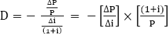
Arnold and North (2008) propose a sensitivity study, which comes from the duration, in order to determine the effects of variations in expected parameters and to provide a measure of the variation in cash flows3. Duration corresponds to the sensitivity analysis that relates to changes in interest rates within a portfolio of bonds. This is the period at the end of which profitability is no longer affected by changes in interest rates because it appears as the discounted average lifespan of all flows (interest and capital). In other words, the duration of a financial instrument is defined as the average lifespan of its financial flows weighted by their present value. So, all other elements being equal, the greater the duration, the greater the risk. According to Macaulay (1938), the duration D that generates cash flow CF is defined as the average duration of repayments of a bond (principal and interest) weighted by its present market value.

where:
- – P: price of bond;
- – i: discount rate.
Therefore, the duration corresponds to the average of the dates that the flows are received, weighted by the weight of each discounted cash flow in all of the flows (the fraction of each term represents the weighting coefficient). The sensitivity S of a bond expresses the relative change in percentage of the price P of a bond for a change in the interest rate i. And so:
Or:
Consequently:
where:
- – P: bond price;
- – S: sensitivity;
- – D: duration.
Duration can be used to find a variation in the bond price given a variation of the discount rate according to Bodie et al. (2004).
The length of the duration indicates how sensitive the price of a bond is to changes in the interest rate. A longer duration means a greater change in the price of the bond as the interest rate moves. To mitigate the risk of interest rate fluctuations, several types of securities can be combined to form a target or optimal portfolio duration. Thus, the valuation of a project V equivalent to a zero-coupon bond is characterized by cash flows CFi and the terminal value VTN assessed over the duration of project N:
where g is the infinite growth rate assuming k > g.
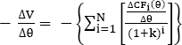
The negative partial derivative of the project cash flows relating to the discount rate gives:

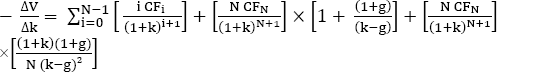
By multiplying equation [2.132] by (1 + k) and by dividing it by [2.129], we obtain the project duration:
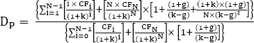
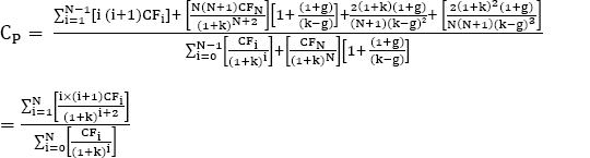
The duration of the project also varies over time if the parameters change. To enter the variation in duration as a function of the discount rate, the “convexity” of a project, CP, is based on the second derivative of the value of the project relative to the discount rate:
The greater the convexity of the project, the greater the variation in duration with a variation in the discount rate. Convexity measures the instability of duration if the discount rate is adjusted. For an infinite horizon similar to [2.129], we have:
The concept of duration can be applied to an “internal” parameter. Also, if we take a project at time i, a function of the internal parameter θ influences the cash flows, CFi (θ). The duration that relates to this parameter therefore depends exclusively on the project itself by its capacity to generate cash flows. We then see a notable difference with the analysis of the duration of the discount rate, which takes into account the cash flows as such and assesses only the effect of its own variation. Thus, equation [2.130] becomes:
The duration of the DPRM project parameter gives4:
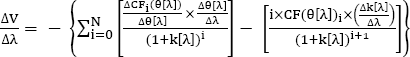
Therefore, suppose that the internal parameter of the model and the discount rate are affected by a common factor, λ, such as inflation. Respectively, [2.136], [2.137] and [2.138] become:
Suppose that the project ends in N years. Let us take:
– OC: operating costs;
– CL: current liabilities;
– CA: current assets;
– WCR: working capital requirement;
– FA: fixed asset;
– AMO: amortizations;
– IT0: initial turnover;
– T: corporate tax rate.
These parameters are measured and expressed as a percentage of sales. Linear depreciation is correlated with turnover (depending on fixed assets):

To find the duration of the internal parameter relative to g, we include it by multiplying the derivative by (1 + g) and dividing by [2.146]. Let A = V(CA) and decompose the equation:
We could add a terminal value if the project had an infinite time or even an initial cost (negative value in the denominator of [2.150]). By considering a variation of the value of the project based on the duration of the internal parameter of the project of [2.150], we get:
2.2.2.2.2. The risk of bankruptcy: risk premium or adjusted growth rate
Shaffer (2006) proposes an extension to the DCF valuation model by considering the probability of bankruptcy5. Empirically, this approach relates more to forecasting premiums on equity, but it improves how risk is calibrated without penalizing the asset’s value or its growth potential. It also explains the irreversible impact of the breakdown of cash flow. We might think that if the risk of bankruptcy is significant when looking only at a time distant in the future (a decade or century away), it would only be considered by a nominal proportion of investors who tend to think in years. However, a significant portion of the present value of cash flows corresponds to the terminal value. For example, assuming an annual FCF growth rate of 3% and a discount rate of 4%, it turns out that 62% of the present value is from FCF generated in more than 50 years6. To the extent that bankruptcy acts as a barrier that absorbs cash flow, there are interdependencies between bankruptcy risk and the valuation to be considered. In the event of bankruptcy, shareholders may receive a residual sum (after having paid off the creditors) and no longer receive continuous flows based on the returns achieved. Shaffer quantifies the impact of this absorbing barrier (which is economically important7) on valuation and shows that it hinders the assumption that an additional linear risk premium exists. The annual probability of bankruptcy, given as a starting point, can be empirically “benchmarked” either by historical reference of the aggregates or by obtaining specific company estimates by applying a statistical model of company bankruptcy.
The analysis ignores other sources of risk, but this does not change the valuation, since the analysis does not assume that investors are risk-averse (that they require a risk premium). The analysis is general and although it could be integrated into a continuous-time model (such as that of Dufie and Singleton (1999)), Gordon’s growth model is used for clarity. Remember that without default risk, the present value of future cash flows V is:
where:
- – ct: cash flow from assets at the start of the year t;
- – k: annual discount rate;
- – c0: initial cash flow.
Cash flows are assumed to grow at the rate g < k.Cash flows can be dividend payments; the infinite time horizon then reflects the fact that stocks have no maturity. Then, the model incorporates the probability p (0 < p < 1) that the asset will default in any given year, which will cancel out subsequent cash flows. Suppose that this probability is independent of t, the risk of bankruptcy following a simple distribution and bankruptcy or survival being characterized by an independent series8. Let us also ignore the possibility that investors will receive a lump sum of liquidation payment in the event of bankruptcy. Under these assumptions, the probability of the firm going bankrupt in year T is equal to the product of p times the probability that the firm survives to year T, or p (1 – p)T. In the absence of bankruptcy, cash flows continue to follow a non-stochastic growth rate g. The expected present value VA of the cash flows is:
where the denominator is greater than that of equation [2.152] for all p > 0 and is therefore strictly positive when r > g (as required by Gordon’s basic growth model). Equation [2.153] corresponds to the valuation of an asset with an initial cash flow c0, which increases at an annual rate g, discounted at an annual rate k, subject to an annual probability of failure p (or maturity, or default irreversible). Equation [2.153] also corresponds to equation [2.152] if p = 0. In other words, Gordon’s valuation of growth without failure is a special case of valuation with a risk of stochastic bankruptcy.
Note that by “correcting” equation [2.152] based on the probability of failure without taking into account the permanent cessation of cash flows in the event of bankruptcy, the annual cash flows per period are replaced by ct (1 – p). We then have ![]() . The numerator is the same as equation [2.153], but the denominator is always smaller, which means that the valuation is greater than the correct calculation of equation [2.153]. And so, this is consistent with the difference between permanent bankruptcy and uncorrelated annual shortcomings.
. The numerator is the same as equation [2.153], but the denominator is always smaller, which means that the valuation is greater than the correct calculation of equation [2.153]. And so, this is consistent with the difference between permanent bankruptcy and uncorrelated annual shortcomings.
This valuation model applied to equity can also be used when valuing the company itself. The main difference is the structure of debt and equity, which affects both the probability of insolvency in each period and the net asset value at the time of bankruptcy. When a company goes bankrupt, it results in losses being incurred by both shareholders and creditors. In addition, liquidation costs are added to the establishment undergoing the liquidation procedure. A comprehensive model of company value must therefore be distinct from the equity valuation model, precisely because of these expected bankruptcy costs. In this case, a comparative analysis is carried out between the assumed liquidation costs and aggregate net worth at the time of bankruptcy. Thus, equation [2.153] can be applied to a firm facing difficulties, but not necessarily in bankruptcy. Such a company is likely to make no gain and pay no dividend – i.e. a situation wherein DCFs are known to provide poor valuations. Severely troubled companies with negative bottom lines do not need to claim a model to identify their difficult situation, and at the time of bankruptcy, the relevant calculation is the present net asset value rather than the risk-adjusted projection of future value. The most useful application of this model therefore concerns companies with a moderate risk of bankruptcy. The impact of low bankruptcy probabilities on the valuation of risk premiums is considerably greater than previously recognized. Thus, taking into account the impact of such a risk is important for all companies. Equation [2.153] can also be used to calculate the ratio of the value of the asset to the current flows generated (Vasset = VA∕c0), which would be consistent with the particular values that k, g and p take, assuming a neutral risk:
where D = g(p -1) + p + k, which corresponds to the denominator k – g of equation [2.153], plus an adjustment for the effect of bankruptcy risk at any time, namely p(1 + g). The price-to-dividend ratio increases with the expected growth rate but decreases with the discount rate and the annual probability of bankruptcy. Note that g and p enter equation [2.153]. This functional formula makes us question whether an additional risk premium or a growth adjustment is sufficient to reflect the impact of the probability of bankruptcy on the valuation of an asset. Consider the convexity of Vasset with respect to p characterized by:
where the sign is established because D > (r – g) > 0. And so, the price-to- dividend ratio is strictly convex at p. Combined with equation [2.154], equation [2.157] establishes that the marginal decrease of Vasset weakens as the values of p increase.
In the DCF method, the integration of risk corresponds either to a downward adjustment of the growth rate used or as an additional constant (risk premium) in the process of discounting. These additional values are used not only to estimate the assets but also to calculate the returns from a given risk profile or, conversely, to deduce the levels of risk involved by the observed asset returns. Therefore, although equation [2.153] is suitable for practical applications, it is necessary to combine equation [2.153] with equation [2.153] if we want to consider an adjusted growth rate G or a premium additional risk R.
To find the expression for the adjusted growth rate of cash flows that incorporates the probability of bankruptcy in the valuation provided by Gordon’s model, k is fixed:
The downward adjustment of the growth rate to be attributed to the risk of bankruptcy is equal to a period of anticipation of the future value of the risk rate (the ratio of the annual probability of bankruptcy to the annual probability of survival): G < g for all p ∈ (0,1) and for k ≥ 0. Moreover, G → g for p → 0.
We can note that G is linear in g ![]() , requiring only one additional term to correct the risk of bankruptcy. The adjustment factor is nonlinear k and p. We thus have:
, requiring only one additional term to correct the risk of bankruptcy. The adjustment factor is nonlinear k and p. We thus have:
Thus, a greater probability of bankruptcy reduces the effective growth rate of returns (see equation [2.160]). And a larger discount rate combines the impact of the risk of bankruptcy on net present value by reducing the effective growth rate (see equation [2.161]). The concavity of G with respect to p can also be evaluated:
And so G is strictly concave at p. Combined with equation [2.160], this result establishes that the downward adjustment of G is greater as the values of p increase.
As an alternative to adjusting the assumed growth rate of cash flows, an additional risk premium R can be calculated to incorporate the risk of bankruptcy. Following this approach, we solve the following equation in order to define the conventional valuation that corresponds to the corrected valuation for the risk of bankruptcy in equation [2.153]:
where the denominator is different from zero for all p ≠ (1 + g)/(k + g + 2). The risk premium is a function of risk-free rate, the growth rate and the probability of failure. By defining E, the denominator of equation [2.164] which corresponds to the basic crude growth rate, 1 + g, minus an adjustment for the effect of bankruptcy risk over time, p(k + g + 2), we find:
where equation [2.167] < 0 if p < 2/3 when r and g are very small positive numbers. R > 0, for a sufficiently small p, although p > ½ can result in R < 0.R → 0 and p → 0. The close correspondence between the risk premium model given historical bankruptcy rates and market risk premiums observed during the same period suggests another use of the model. Given the values of k and g, equation [2.164] can be solved for p as a function of the observed risk premium on the equity of a particular firm. If the market risk premiums correctly reflect the risk of bankruptcy, the implied value of p provides a convenient way to summarize information about this risk embedded in the market price of the company’s shares:
The model can be extended to calculate the stock value of a company whose growth rate changes drastically. Cash flows after this transition would either remain at the level observed before the period or increase at a different rate. For example, a company has a phase of rapid initial growth, followed by a downturn phase. If the company’s cash flows grow at a rate g until period T and then remain constant thereafter, the present value of the cash flows if 0 ≤ g <k is:
If the transition occurs with the probability p during a period t, then the value of equity that corresponds to the value of discounted cash flows is:
Equation [2.170] is a return to the Gordon valuation, co (1 + k)∕(k – g), as a special case if p = 0. We may also consider either an additional risk premium or an equivalent constant growth rate to adjust the valuation to be equal to this expression. The effective discount rate R (k + additional risk premium), to define co (1+ R)∕(R – g) equal to equation [2.170], can be calculated as follows:
We can calculate an equivalent constant growth rate G leading to the same valuation while discounting at the risk-free rate by co (1 + k)∕(k – G):
Therefore, if a firm’s cash flows show a stochastic transition from positive growth at rate g to a zero growth rate, the valuation of these cash flows is given by equation [2.170] ; the same valuation can be obtained by substituting either R from equation [2.171] or G from equation [2.172] to the Gordon growth model. This analysis can be generalized in the case of positive growth after period T but at a different rate γ. The present value of the cash flows is:
If 0 ≤ g < k, the expression reduces equation [2.169] to a special case if γ = 0.
With a transition probability of the growth rate g to γ, the present value associated with equation [2.173] can be calculated analogously to equation [2.170]:
which reduces equation [2.153] if p = 0 or γ = g and equation [2.170] if γ = 0. The adjusted discount rate (or growth rate) to obtain the same valuation using Gordon’s growth model is:
And these expressions reduce, respectively, equations [2.171] and [2.172] for γ = 0. Therefore, if a company’s cash flows show a stochastic transition from one growth rate to another, the valuation of these cash flows is given by equation [2.174]; the same valuation can be obtained by substituting either R from equation [2.175] or G from equation [2.176] to the Gordon growth model.
Consequently, this analysis justifies the use of either the growth adjustment or an additional risk premium and demonstrates the responsiveness of these two terms to three exogenous factors (risk-free rate, expected growth rate of cash flows and probability of periodic failure).
Reviews in the literature are focused on theoretical adjustments vis-à-vis optimizing the financial structure and beyond this, on valuation methods by discounting cash flows – adjustments based on conceptual parameters. It therefore seems interesting to analyze studies that address the performance of valuation methods according to specific contexts. Indeed, certain methods could prove to be more appropriate to the detriment of others when it comes to valuing a transaction with leverage or a company with particular characteristics in terms of structure, size, type of activity or the particular stage of its development.
2.3. Contextual impacts and adjustments
Kaplan and Ruback (1995) compare performance in terms of market anticipation according to different valuation methods, based on the APV method and on the EBITDA multiple, from a sample of companies that have undergone management buyout operations and recapitalizations. In this context, they recommend retaining a high risk premium and generally favoring discounting cash flow methods.
By focusing on the sector multiples method, Lie and Lie (2002) find that overall the asset multiple provides better estimates and that the EBITDA multiple provides better estimates than the EBIT multiple. In other words, allocations and takeovers would adversely affect the enterprise value. Alford (1992) carries out an important study about samples and variety of tests. He concludes that the P/E multiple provides more precision when benchmarks are chosen on the basis of industry and when businesses classified as such have similar financial returns and asset values. It is in this sense that Zarowin (1990) and Kim and Ratter (1999) extend their research on the performance of the P/E multiple according to different contexts.
Hotchkiss and Mooradian (1998) focus on company takeovers in the situation of bankruptcy. According to them, the prices paid, which are calculated from the revenue or asset multiple, are on average 45% lower than the corresponding transactions between companies operating in the same industry that are in good health. In other words, the two researchers believe that this result comes from the information imbalance that exists in such situations. Gilson et al. (2000) compare the market value for shares of listed companies that are restructured after a situation of bankruptcy with their discounted cash flow valuations which are calculated from their reorganization plans. Significant disparities can be noted depending on the time that has elapsed since the restructuring. If the valuations do not correspond to reality, these differences are not, according to the researchers, linked to errors in calculation. Rather, they are due to problems that relate to the quality of information that is available during the administrative process that has been initiated in order to declare the situation of bankruptcy (replacing the market). Along with this, they are due to strategic biases, namely agency conflicts, which benefit certain parties such as creditors or management when the value is underestimated. In this context, valuation is used more for strategic purposes and becomes a determining element in negotiations.
Damodaran (2009) tries to propose an appropriate method to value a young company. He affirms that valuation must be linked to sales or to the net result, incorporate a target rate of return and focus on short-term forecasts (2-5 years of business plans, coinciding with the resale forecast for the benefit of a venture capital fund).
2.3.1. Leverage transactions
The principle of leverage buy out (LBO) consists of acquiring a target company by an ad hoc takeover holding company that is financed in large part by debt. The equity of the holding company alone represents a lower investment than that which would have been necessary to buy shares of the target company. The leverage effect can thus be put into practice by considering that the financial profitability of the target is greater than the cost of the debt. The holding’s acquisition debt is then repaid thanks to dividends that are paid by the target and, to a lesser extent, thanks to the cash generated by the exit from the LBO. For the latter to work, it is necessary for the target to operate in a mature market that is synonymous with moderate investments, thus facilitating the payment of dividends. The latter is also a function of the target’s debt level, which at a reasonable level allows it to allocate most of its cash to the takeover holding company.
In addition, it is recommended that visibility is as clear as possible, as this will make the business plan and forecasts more reliable when it comes to the exit of the investment funds when the target is introduced to the stock market or it is sold to an industry or to another fund. Initially, the sale price of the target is capped at the maximum amount of finance likely to be raised by the takeover holding company. Therefore, the value of the target is no longer an assumption but an outcome. It corresponds to the maximum amount of funds that can feasibly be raised by the takeover holding company in the form of capital, subscribed by the investment fund(s) and the acquisition debt raised from banks. In fact, determining the value of the target means structuring the financing of the holding company. Acquisition debt, for its part, is directly linked to the expected profitability of the target. It is adjusted by incorporating the idea that repayment will take place over a period of 7–9 years through the dividends distributed by the target to the holding company. The profit distribution rate of the target is assumed to be 100% as soon as the LBO is set up. In addition, the debt is calibrated so that the holding company maintains a cash flow that is in slight excess, so as not to generate additional financing needs. Finally, it is necessary to respect financial ratios or covenants that allow lending institutions and financial bodies to control the progress of the LBO. Equity is set at a level which ensures that investment funds receive an internal rate of return of about 20–30% in 3 years. This is on the assumption that the fund will exit by IPO, by a sale to an industry, or to another fund on the basis of a multiple of EBITDA or EBIT, according to market conditions at the time of setting up the LBO. The value of the target is, in practice, slightly lower than the sum of the values of the shareholders’ equity and the debt of the holding company, because the latter must also finance various costs of about 3–4% of the holding value of the transaction (fees for lawyers, advice, legal, accounting and tax audits and payment of a commitment commission on the acquisition debt), which are all linked to the process of acquisition.
Kaplan and Ruback (1995) attempt to compare the market value of a sample of 51 characteristic management buyout and recapitalization transactions with valuation methods based on discounting cash flows using the APV method (adjusted present value) and on the EBITDA multiple (thus excluding the P/E multiple due to the fact that companies have different financial structures). The empirical problem of their study is to understand whether the parametric assumptions of the APV methods specific to the company having undergone these types of leveraged transactions provide better results than the incorporation of expectations that are contained within the comparables methods. Their work therefore begins with the definition of different valuation models using the APV method initially developed by Myers (1974). They consider three different weighted average costs of capital distinguished in this by their respective beta: the first is calculated from the beta of the company, the second from the sector beta and the third from the market beta (this is that of the sample). In addition to trying to compare the valuation details of these same cash flow discounting methods, they also want to make comparisons with estimates based on the EBITDA multiple. Likewise, they define three comparables methods: the first based on a benchmark of comparable companies, the second resulting from comparable transactions and the third resulting from transactions that have been carried out in the same industry between comparable companies.
The median – derived from APV company valuations based on the company beta – is 6% above the trade value. Therefore, we see that valuations using the beta of the sample (market) are closest to the transaction values in terms of both median and mean. We can also see that the standard deviation is the smallest, which is proof that the variations are smaller with this method. Regarding the multiples method, in view of the median, we would recommend a priori to use an EBITDA multiple from a sample of comparable transactions between companies in the same industry. However, by analyzing its standard deviation, we note that this type of sample provides the most disparate values. Moreover, Kaplan and Ritter express that the number of companies that combine these two criteria and therefore constitute this type of sample is limited. Indeed, 13 of the 51 companies in the overall sample could not be grouped together in a repository. We can therefore suspect that it is difficult, if not impossible, depending on the period and sector of activity, to constitute this type of sample in practice. The work of the two researchers can be extended by presenting the error estimates as a function of the risk premiums applied.
Table 2.2. Errors (the definition of the error results from the calculation ![]() ) between the values of the transactions carried out and those of the different valuation models
) between the values of the transactions carried out and those of the different valuation models
| Methods based on different WACCs | Methods based on different samples | |||||
| Company beta | Sector beta | Market beta | Comparable companies | Comparable transactions | Comparable transactions between comparable companies | |
| Median | 6% | 6.2% | 2.5% | -18.1% | 5.9% | -0.1% |
| Average | 8% | 7.1% | 3.1% | -16.6% | 0.3% | -0.7% |
| Standard deviation | 28.1% | 25.1% | 22.6% | 25.4% | 22.3% | 28.7% |
| Median beta | 0.81 | 0.84 | 0.91 | |||
Table 2.3. Variation in valuation errors depending on the size of risk premiums applied to the different valuation methods
| Methods based on different WACCs | Methods based on different samples | |||||
| Median risk premiums | Company beta | Sector beta | Market beta | Comparable companies | Comparable transactions | Comparable transactions between comparable companies |
| 5% | 25% | 24.8% | 21.2% | 30.1% | 29.2% | 26.6% |
| 6% | 16.4% | 17.7% | 13.6% | 25.2% | 23% | 20.3% |
| 9% | -2.3% | -3.1% | -7.6% | 20.3% | 17% | 17.4% |
The results indicate that it makes good sense to use a high risk premium to obtain a more accurate valuation. For example, with the APV method based on the beta of the company, applying a risk premium of 6%, the median of the valuation error is of the order of 16.5%, while when the premium of risk is 9%, the median indicates that the valuation underestimates the value of the transaction actually carried out by only 2.3%15. To refine their analysis, Kaplan and Ritter present error histograms for each method. They find that APV methods based on an industry or market beta show a greater tendency to provide valuations below 15% error, while methods based on the EBITDA multiple give more uniform results. In other words, about 60% of the valuations carried out by one of the two APV methods mentioned above are less than 15% of the value of the transaction carried out, while the percentage of the valuations resulting from the multiple of EBITDA based on a benchmark of comparable companies or transactions – for this same criterion of precision regarding the value of the (i.e. 15%) – relate to 37 and 47% of the valuations, respectively16. Therefore, Kaplan and Ruback favor discounted cash flow methods for three reasons. They tend to provide more valuations below 15% accuracy. In addition, the two best comparables methods studied here use transaction repositories, and in practice, their scope is far too small, unlike the discounted cash flow methods. Finally, they estimate their prediction of perfectible cash flow, and therefore, in practice, the financial bodies with more information can adjust the valuations more effectively using this type of method.
Even though, in theory, the most precise valuation of the company is part of a medium- and long-term development perspective, i.e. by applying the DCF method, in practice, it can be found to be biased and unreliable. Indeed, it may be difficult depending on the context, to accurately anticipate future flows and/or to assess a discount rate that takes into account the optimal amount of risk. This is the reason why analysts and investment bankers may prefer to use – or at least provide in addition – a valuation based on the market comparables method. Also, it seems interesting to ask if empirically there may or may not be a multiple that provides more precision around the value of the company in absolute terms, depending on a specific context or market sector.
2.3.2. Stock market multiples: from the impact of structures to anticipating profitability
Amir and Lev (1996) study valuations in the telecommunications industry and show that the first factor that impacts enterprise value is the population of a franchise territory and not financial variables. Thus, there is no answer as to which multiple should be favored over another: the relevance of the value that comes from the P/E can be as well established as that found from the asset multiple. Thinking more globally, Lie and Lie (2002) constitute a sample of more than 8,600 companies that they value using 10 different multiples. Then, they estimate the errors between their calculations and the market values. Among the multiples based on enterprise value and observing the percentage of valuations below 15% of errors compared to the market value, it turns out that the multiple of assets provides the best estimate (35%) and the multiple of turnover the least precise estimate (23%). Moreover, from the same perspective, the multiple of P/E based on forecast results is more precise than when it is calculated from book values, according to the conclusions of Kim and Ritter (1999) developed below. In addition, the EBITDA multiple provides better estimates than the EBIT multiple. Thus, it appears that allocations and operating reversals distort value, as depreciation schedules do not accurately reflect deterioration in asset value.
Lie and Lie then separate financial corporations from non-financial corporations and analyze them. This choice of creating two separate samples is justified by the liquid asset nature of the assets of financial corporations, which facilitates evaluation compared to non-financial corporations. In line with the findings of Alford (1992) below, valuations of non-financial firms are more accurate when their size is substantial. Indeed, the smallest companies have more erratic results, while the large structures can be considered as a large portfolio of projects. In addition, regardless of the size of the structure, the multiple that confers the most faithful value to that which relates to the market is the assets multiple, and the one that confers the least is the turnover multiple. For example, Lie and Lie find that within a sample of medium-sized companies (the book value of assets ranging from $100 million to $1 billion), the valuations derived from the revenue multiple are 20% below the 15% error, compared to the market value when looking at this same criterion, the valuations that result from the assets multiple are at 30%. The dominance of the asset multiple is all the more obvious for company valuations with low (or even negative) EBITDA, relative to the book value of their assets. For companies with significant EBITDA compared to the book value of their assets, how precise the different multiples are related to whether it is P/E, asset multiple, EBITDA or EBIT; valuations located at less than 15% of the market value are about 25%. The performance of the asset multiple over other multiples becomes most pronounced when it comes to studying financial companies. The median valuation error underestimates the market values of major financial companies by 1% (the book value of assets is greater than $1 billion), and 83% of these valuations are within 15% error relative to market value.
Apart from the distinction made between non-financial and financial corporations, the Lie and Lie study does not look at specific contexts. Milicevic (2009) even shows that if in practice in order to compose their sample, investment analysts and bankers consider companies that are in the same sector of activity, they will always reside within the same branch of activity, albeit in different classification systems. In addition, the incorporation of foreign companies that follow different accounting and regulatory rules generates inaccuracies with regard to forgetting that some companies operate in different sectors, which alters a representative identification of the benchmark. In addition, the theoretical justification that companies in the same sector should have similar rates of profitability, growth and risk profiles weakens the credibility of the results obtained. Milicevic also mentions limitations faced by the transaction multiples method. Numbers provided within the same sector in a limited space-time turn out to be rather concise, while not providing satisfactory statistical data for analysis each time. In addition, market conditions are constantly changing, which can discredit the premiums for transactions that are selected for valuation. It is then a question of knowing how to identify a suitable sector of activity and understand what is the ideal size of a repository. After defining them, we must ask ourselves whether they meet the comparison conditions as such, or whether it makes sense to make certain adjustments.
It is in this sense that the empirical work of Alford (1992) attempts to detect a level of consistency when determining the benchmark of companies when the valuation is carried out by the P/E multiple. Even though Boatsman and Baskin (1981) and then LeClair (1990) had carried out empirical studies on this subject before him, the fact remains that their tests had certain methodological limitations. In fact, for their P/E test, Boatsman and Baskin used two kinds of sample for comparable companies: one based on companies that belong to the same sector of activity and the other on companies that belong to the same sector of activity with similar 10-year earning growth rates. The conclusion of their analysis leads us to consider that composing a sample of companies on the basis of the criteria of the second benchmark provides makes the valuation more precise. However, the two researchers focused on examining 80 companies over a year based only on the assessment of a single comparable company. LeClair, for his part, tests the P/E multiple with a sample of 1,165 companies that are comparable in terms of industry. He classifies them into three subsets, distinguishing them by criteria that relate to their net results (which are all positive). We thus can find a repository of companies whose results for the previous year were similar, a benchmark of companies whose average profits over 2 years are of the same type of magnitude and a benchmark of companies whose share of profits that are related to tangible and intangible assets is substantially similar. LeClair considers a different discount rate for each source of earnings. He concludes that the sample of companies with similar 2-year average net results provides the most accurate value, yet he does not test to see how the significance in the precision of the three measures is different.
Alford’s influence lies in the breadth of his study. He carried out these tests on 4,698 companies in three different years (1978, 1982 and 1986) by constituting seven benchmarks which are made up of company multiples17 that belong to various sectors of activity. He therefore studied – in addition to the criteria linked to industrial comparisons as such – potential valuation convergences between companies that only have equivalent asset values and/or financial returns. Therefore, he examines seven potential sets of comparable businesses:
- – the companies that constitute the whole of the sample, i.e. the market of the companies studied;
- – companies that belong to the same sector of activity that it defines using the standardized classification of American industries18;
- – companies in the sample with similar asset values;
- – companies in the sample with close financial returns;
- – the combination of companies that belong to the same sector of activity and have a similar asset value;
- – the combination of companies that belong to the same sector of activity and which have close financial profitability;
- – companies that have both an asset value and a similar financial profitability (without being from the same sector of activity).
The methodology is as follows: after having designed seven subsets, each company is valued by multiplying net income by the “categorical” P/E, which is then calculated. The “absolute prediction error”, ei,t,, is then estimated, which is equal to:
where:
- – Pi,t: value of share i found by the multiple P/E method at time t;
- – pi,t: current (real) value of share i at time t.
Finally, the mean of the median values is measured for the absolute prediction errors19 for each subset. It is then concluded that the P/E tends to be more precise when comparable companies are chosen on:
- – the basis of their sector of activity. In this case, the mean of the median values for the absolute prediction errors is 24.5%;
- – the combination, to a lesser extent, of the business sector with similar financial returns. In this case, the mean of the median values for absolute prediction error is 25.3%.
Alford’s findings confirm a financial reality. It seems theoretically obvious that the financial profitability of the companies that make up the sample and that of the target must be of the same order of magnitude. Indeed, by multiplying the sector P/E by the net income of the company to be valued, we can obtain an estimate of potential market capitalization where:
where:
- – MC: market capitalization of the company being valuated;
- – NR: net result of the company being valuated;
- – EBIT: operating result of the company being valuated;
- – i: cost of the net debt of the company being valuated;
- – D: net debt of the company being valuated;
- – t: corporate tax rate.
Consequently, the sector P/E [EBIT(1 – t)] would represent the enterprise value and the sector P/E [iD(1 – t)] would represent net debt. In practice, this equality is fair if and only if:
We also know that:
So:
where Rf is the sector financial profitability.
In other words, if theoretically it seems wise to value a company by applying the sector PER to its net profit, the use of this method in practice implies that in order to achieve a greater degree of accuracy, the companies within the sector of activity have almost identical financial returns. Indeed, if the sectoral financial profitability is greater than the cost of the after-tax debt of the company to be valued, the latter’s equity would be overvalued because the debt would be undervalued, and vice versa, if the sectoral financial profitability is lower than the after-tax cost of debt of the company to be valued, equity would be undervalued because the debt would be overstated. In accordance with the Dupont de Nemours formula20, this difference in profitability can be explained through a differential in the net margin rate, the asset turnover rate and/or the use of leverage.
When a company’s stock market status is constant, so is the P/E21. Indeed, it would seem a priori that if the stock price increases, the P/E in turn increases, but this would mean that we are forgetting that it is because, going upwards, the profit per share increases such that the market passes this expectation onto the price of the stock exchange. It is in this sense that the work of Zarowin (1990) responds empirically, using a sample of 175 companies, to the possible factor(s) that impact(s) the P/E. His study spans 5 years (from 1964 to 1968 inclusive). The companies are chosen so that their whole more or less replicates the market. To do this, he relies on an annual average beta that ranges from a minimum of 0.988 to a maximum of 1.054. He then defines two kinds of P/E22: the first is based on an observed benefit and the second on a “normalized” profit. The latter results from the incorporation of forecasted growth rate and risk according to the model of Litzenberger and Rao (1971). Thus, the second P/E seeks to ignore any cyclical accounting adjustments and optimizations. Zarowin then sets up 15 portfolios of companies of the same size. Classification is carried out on the basis of similar P/E. He then observes, for each year, the correlation that arises from the 15 portfolios by studying the P/E variations. He finds that the P/E correlations between the different portfolios each year are strong (close to 1) regardless of whether they are observed or normalized P/E. The results run counter to the conclusions developed by Beaver and Morse (1978), for whom variations in P/E are essentially justified by variations in accounting methods that result from considering inventory valuation rules or from taking into account the level of depreciation. Indeed, according to Zarowin’s results, if the differences between the accounting methods had been the main cause of the differences in the values of P/E over time, their failure to take them into account – i.e. to consider a normalized P/E normalized “freed” from accounting constraints – should have resulted in more decorrelation (close to 0).
Zarowin completes his study by reconciling the normalized and observed P/E through regression calculations. The average of the correlation coefficients established over the years of study is 0.85, which indicates that the accounting methods are at most responsible for the variations in current P/E at 15% on average. Tojustify variations in P/E, Zarowin performs regression calculations between short-term and long-term forecasted growth, beta and observed P/E. He notes that the long-term forecasted growth justifies 70% of the P/E realized, while the average coefficient of long-term forecast growth is six times greater than the growth coefficient that is actually achieved. According to him, the explanation is that the long-term growth forecasts are influenced by the observed P/E and not the other way around, namely that the multiple is affected by any forecast growth. Moreover, Zarowin’s point is confirmed when he presents the correlations of the long-term forecasted growth rates of the samples across the years of study. They turn out to be close to 1. An interesting conclusion that can be deduced from this work is the non-significance of the beta, whereas the risk associated with the growth forecasts seems to be a second factor that could affect the P/E. The average correlation between beta and predicted long-term growth is 0.58. These results are in line with the tests undertaken by Tinic and West (1984) on the equilibrium model of financial assets and with those of Liu and Ziebart (1994), who examine the transversality of the variabilities of PER23. They uncover a significant relationship between this ratio and growth, dividend payout and company size. On the other hand, they also emphatically perceive that there is no relation between the PER and systematic risk. To complete this analysis, it would be interesting to identify the specific risk factors used by the market and to test, finally, the impact of interest rates on the P/E.
By adjusting its benchmark as Alford did, the reliability of the P/E cannot justify all valuations. In accordance with what has been developed previously, it is so to speak weak to rely on this single multiple to valuate, for example, a company that wishes to introduce its capital on the stock market. Indeed, in this case, the financial structure of the company varies appreciably from that of the companies already listed, which operate in the same sector without taking into account that their respective value of the assets is appreciably different – fundraising that can justify the IPO. In addition, when evaluating a company that wishes to make all or part of its capital public, the DCF method can definitely be ruled out because it is too imprecise. Predicting future cash flows involved may be too difficult, if not impossible to do. If we refer to the work of Varaiya et al. (1997), during a stock market listing, it would be necessary to recommend the use of the multiples method on the basis of accounting information. However, the work of Kim and Ratter (1999) – which aims to provide empirical evidence for the accuracy of multiples in when valuating an IPO company – suggests that, without adjustments, there are too many inaccuracies when we rely solely on historical accounting data. Theyjustify these valuation errors by asserting that listed companies in the same industry have such variable P/E relative to each other that, on that basis, any price can be justified. On the other hand, they suggest that by turning to forecast earnings (to which a growth rate and profitability rate are applied) in order to calculate the P/E, the accuracy of the valuation would improve significantly. They decide to extend their study to other multiples: market value over book value of equity, stock market price over turnover, enterprise value over turnover and enterprise value over operating cash flow. To carry out their research, they make up two repositories of 190 companies that have gone public less than a year after the announcement of their preliminary offer price. The first groups together all recent IPOs from the same industry24 and whose data is only accounting and historical. The second brings together IPOs of comparable companies that have been chosen by classifying a company that specializes in IPO valuation25. In this second sample, notably, the data is forecast.
Table 2.4. Error between current values of multiples and predicted values of multiples according to the criteria of the first repository (accounting data)
| Multiples | Absolute prediction error | Percent regression of valuations included at least 15% of the current multiple | ||
| Mean | Median | Offer price | First quotation at close | |
| P/E | 56.5% | 49.9% | 14.2% | 17.4% |
| Market value/book value of equity | 33.1% | 30.6% | 27.4% | 22.1% |
| Stock market price/turnover | 62.4% | 51.5% | 13.2% | 12.0% |
In the best-case scenario, when using a valuation by the multiple of the market value of equity over its book value, approximately 27% of the offer price valuations are less than 15% of the actual traded value. This same method overestimates the transaction value by an average of 33.1%. In addition, the accuracy of all multiples (based on accounting data) decreases at the end of the first day of trading.
Table 2.5. Error between current P/E multiple and forecast P/E according to the second criteria of the second standard
| Earnings per share used26 | Absolute prediction error | Regression of the percentage of valuations included at least 15% of the current P/E | |
| Mean | Median | ||
| Historical accounting data at 1 year | 55% | 52.1% | 15.4% |
| Forecast data for the current year | 43.7% | 40.1% | 18.9% |
| Forecast data for the next fiscal year | 28.5% | 22.2% | 36.4% |
Table 2.6. Error between the current P/E and forecast P/E multiples between young and old companies of the sample according to the second standard
| Earnings per share used | Absolute prediction error | Regression of the percentage of valuations included at least 15% of the current P/E | |
| Mean | Median | ||
| Forecast data for the current financial year (young companies) | 31.9% | 26.2% | 29.2% |
| Forecast data for the current year (old companies) | 23% | 18.8% | 40.8% |
The more the valuations by the P/E are based on forecast data over time, the more precise they become. The forecast data for the following fiscal year has the lowest mean and median errors and more than a third of within this section provide valuations below 15% of the current value of the P/E.
By distinguishing the “young” from the “old” companies, we find that it is easier to make a better assessment of the latter over the former.
Table 2.7. Error between the current value of the multiples and the predicted values of multiples according to the criteria of the second benchmark
| Absolute prediction error | Regression of the percentage of valuations that are included at less than 15% of the current multiple | ||
| Mean | Median | ||
| Economic value of equity/turnover | |||
| Historical accounting data at 1 year | 56% | 46.3% | 13.3% |
| Forecast data for the current year | 54.6% | 44% | 15.4% |
| Enterprise value/turnover | |||
| Historical accounting data at 1 year | 52.8% | 42.6% | 16.1% |
| Data | 52.1% | 41.8% | 13.3% |
| Enterprise value/operating cash flow | |||
| Historical accounting data at 1 year | 43.2% | 37.5% | 20.3% |
| Forecast data at the current year | 41.6% | 34.1% | 21.7% |
Table 2.8. Error between the current turnover multiple and the forecasted values of the turnover multiple that incorporates a profitability multiple and growth multiple according to the criteria of the second benchmark
| Turnover used | Parameter estimates | Absolute error prediction | Percentage regression of valuations within 15% of the current multiple | ||
| Profitability multiple | Growth multiple | Mean | Median | ||
| Historical accounting data at 1 year | 0.171 | / | 50.3% | 40.4% | 18.2% |
| Forecast data for the current year | 0.218 | 0.199 | 48.8% | 40.1% | 18.9% |
The multiple that is most precise is the one that relates enterprise value to operating cash flow. Indeed, the mean and the median are the lowest, and the regressions for the valuation percentage included within 15% of the current multiple are the highest. Furthermore, the results confirm that the forecasted values confer more accuracy. Kim and Ritter also perform tests on these multiples by separating young from old companies. They come t the same conclusions about whether the oldest companies provide the best valuations: the multiples of the oldest companies that relate enterprise value to operating cash flow are 38%, below 15% of the present value of this same multiple.
The two researchers finally adjust their turnover multiple to apply it to the aggregate of the company undergoing its IPO. By incorporating the factor of profitability in addition to the factor of growth (when it comes to forecast data), we have:
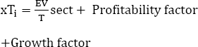
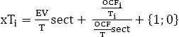
where:
- – xTi = multiple of turnover to be applied to company i which is undergoing valuation (going public);
- –
 of sectoral turnover;
 - –
 of operating cash flow to the turnover of company i to be valued (going public);
 - –
 of operating cash flow to sectoral turnover;
 - – 1 if Δ Ti between year n and n – 1 > Δ Tsect between year n and n – 1;
- – 0 if Δ Ti between year n and n – 1 < Δ CAsect between year n and n – 1.
The turnover multiple gives more precision. Indeed, based on forecast data for the current year, the coefficient for the profitability factor of 0.218 associated with the t-statistic of 4.18 suggests that a 20% premium should be offered to companies that are two times more profitable than the average. In addition, the growth factor with a coefficient of 0.199 also confirms that a premium of 20% must be considered for high-growth companies that list their capital on the stock market. Kim and Ritter’s results reflect a certain practice: the premium offered generally ranges between 10 and 20%. The latter that investment bankers add to the initial offer price when using accounting information is the result of any additional information they have on market expectations.
The P/E is an appropriate method for valuating companies with similar financial structures, the benchmark of which can be optimized by setting it up alongside companies in the same industry with similar asset values. In addition, multiples provide appropriate valuations during an IPO. However, it seems particularly difficult to express a value in specific contexts such as in the presence of companies with significant intangible assets or during a situation of bankruptcy due to administrative and strategic biases punctuating the procedure.
Lie and Lie (2002) find in their study that companies with activities that relate to advanced technology or with significant research and development activities can be particularly difficult to evaluate. Indeed, a large proportion of their value lies in future growth opportunities. In addition, the high degree of expenditure on research and development reduces the operating result, even though the latter can be synonymous as future investments. Thus, when relying on the multiples method which is based on income statement aggregates, the estimate is likely to be skewed. For example, by isolating the 27 “dot-com” companies from their sample, Lie and Lie find that no valuation is less than 15% of the market value of the companies in question, according to the turnover multiple and the assets multiple. They note that only two of them have positive results. The results are scarcely more precise when they apply the multiples method to pharmaceutical companies and groups where research and development expenses exceed 10% of the book value of the assets. They note, however, that the most precise multiple is that of operating profit, unlike more general cases. Therefore, the multiples method is limited when it comes to valuing companies with growth potential and holding intangible assets in large quantity.
Valuation has a central place in the negotiations of bankrupt companies. Indeed, the estimated value of the business in this situation determines the value of the assets to be distributed among the different parties to allow payments and collections. However, bankruptcy is an administrative process and the factors that lead to a reliable estimate of value in a normal market process are absent. In addition, it is difficult for analysts to rely on past bankruptcy situations as they are still too rare to be able to make predictions after the fact. The valuation is therefore more complex and less precise.
According to Damodaran (2009), a young company is characterized by the absence of historical results, a phase of growth that is still to be initiated, low turnover, significant losses linked to operations, dependence on private capital that entails power dynamics, few liquid investments and a very low survival rate. According to Watson and Everett’s study (1996) of nearly 5,200 Australian start-ups, 64% of them fail within 10 years, the annual bankruptcy rate being 9%. Thus, the very characteristics of young companies lead us to consider problems inherent in the process of valuation.
2.3.3. Two delicate contexts for valuation: the bankruptcy situation and the start-up company
American legislation regarding the administration of bankrupt companies, through Chapter 11, regulates bankruptcy circumstances by promoting the continuity of the company. The objective is to save jobs and preserve the economic system, while leaving room to maneuver for a company restructure. Chapter 11, however, emphasizes negotiation. The reorganization plan is based on an estimate of the value of the company to be restructured. The management of the bankrupt company retains control throughout the process, with an exclusive right to initiate the reorganization plan. Disagreeable creditors can vote against the plan or collect more complainants to influence the vote. They can also lobby for an alternative value to be considered, form an official committee or link up with management to develop a better plan that serves their interests. In some cases, when the plan is based on a valuation that is low enough to empower senior debt holders, the latter gain the so-called support of management by offering them jobs, stocks and/or options in the reorganized company. Creditors can ask the court to withdraw management exclusivity from the management of the bankrupt company and file a concurrent reorganization plan. Alternatively, they can request a formal valuation hearing. The most common reason for requesting an assessment hearing is to estimate whether the reorganization plan is “fair and equitable”27. In practice, appraisal hearings and competing plans are relatively rare for large public companies that find themselves in bankruptcy. In general, cash flow forecasts and the values they imply derive from legal actions that relate to diverging economic interests.
Hotchkiss and Mooradian (1998) examine the characteristics of 55 transactions of bankrupt companies that were taken over by listed companies and reconcile their results with 55 other transactions carried out between healthy companies. They find that 66% of bankruptcy takeovers are carried out by companies that have at least one type of activity in common28. By way of comparison, Kaplan and Weisbach (1992) carry out a similar study around acquisitions of companies that do not find themselves in a situation of bankruptcy, and their results indicate that the offeror and the target (with at least one type of activity in common) represent only 33% of transactions. To measure the correlation between an acquisition, Hotchkiss and Mooradian follow the methodology used by Kaplan and Weisbach based on the American classification of SIC according to the Standard and Poor’s register. That is to say, an acquisition is linked to three levels of figures if one of the four activities, which is the most important to the acquirer and the target (classified according to turnover), correspond to this same level of code. To complete their analysis, Hotchkiss and Mooradian note that, for a healthy number of transactions, the target and the acquirer have previously entered into a relationship. This is the case when, for example, the offeror already owns the assets of the target.
As a result, and knowing that the target and the acquirer operate in related activities, there is an information asymmetry problem in the market, which has the consequence of dissuading potential offers from less well-informed companies. This therefore justifies that targets in default are often bought by companies in the same industry. However, this does not prevent there from being more competitive bidding than for transactions between companies that are not in a situation of bankruptcy. In their sample, 18 of the 55 buyout transactions (32.7%) of bankrupt companies had multiple offers from potential buyers, while only 11 ofthe 55 transactions (20%) between “healthy” companies came across such a multitude of propositions.
The work of Bradley et al. (1988) and Bange and Mazzeo (1997) also supports this observation. Indeed, the former find multiple offers for 73 ofthe 236 transactions studied (or 31%), and the latter find multiple offers for 103 of the 436 transactions studied (or 23.6%). In addition, the relative size of targets in the situation of bankruptcy is on average 25.8% of that of the acquirer, based on total assets and 30.2% based on total sales. The conclusions of Clark and Ofek (1994) that also concern the study of a sample of mergers are equivalent.
Table 2.9. Characteristics of bankruptcy buyout transactions compared to two benchmarks (EV: enterprise value; turnover; VcA: book value of assets)
| Mean | Median | |
| Turnover multiple | ||
| EV of the target company in the situation of bankruptcy/ | 1.1 | 0.4 |
| turnover | 1.6 | 1.1 |
| Median EV of a sector of activity/turnover | 2.3 | 1.1 |
| EV of transactions between “healthy” companies/turnover | ||
| Asset multiple | ||
| EV of the target company in the situation of bankruptcy/VcA | 0.7 | 0.5 |
| Median EV of the sector of activity/VcA | 1.3 | 1.2 |
| EV of transactions between “healthy” companies/VcA | 1.9 | 1.2 |
| Price paid in relation to the value that comes from the benchmarks | ||
| Price paid/turnover multiple of the sector of activity | 45.1% | 60.5% |
| Price paid/turnover multiple of transactions between “healthy” | 43.5% | 68.8% |
| companies | 45.7% | 64.7% |
| Price paid/asset multiple of the sector of activity | 40.2% | 59.6% |
| Price paid/asset multiple of transactions between “healthy” companies |
The multiples of target companies in bankruptcy are lower than the other two benchmarks, and the asset multiple is lower, which even leads us to undervalue a company that finds itself in this situation. The prices paid (which are calculated on the basis of the turnover multiple or assets multiple) to buy out bankrupt companies are, on average, 45% lower than the corresponding transactions between healthy companies in the same sector of activity. In other words, even though the prices paid are generally lower compared to the two benchmarks considered, the asymmetry of the information that resides in the market will dissuade companies that do not belong to the same industry.
Gilson et al. (2000) compare the market value of the shares of 63 public enterprises restructured after a situation of bankruptcy with their estimates from projections of their cash flows and their reorganization plans29. To the extent that practitioners suggest that the first share prices after the restructuring plan may experience downward trends as the company’s creditors seek to sell the shares they received under the terms of the restructuring plan, the three researchers examine valuation errors based on the discounted market value of equity at 1 month, 3 months and 6 months after the date of the first listing of the share, following the restructuring plan. The distribution mechanism of shares under a restructuring plan is not the same for the whole sample of companies. Eberhart et al. (1998) convey in their work the problems posed by determining the post-bankruptcy stock price. In this way, it so happens that the pre-bankruptcy share is canceled and a new issue takes place or the old share remains and an issue is added. Valuations are based on the DCF method and the comparables method. Indeed, according to the work of Scarberry et al. (1996), these methods are widely used in practice. Regarding their method of discounting cash flows, Gilson, Hotchkiss and Ruback do not depend on using free cash flows but rather on capital cash flows (CCF). The difference between the two methods is that CCFs measure the money available to all holders (and lenders) of capital and include tax savings on financial interest and other tax benefits. In addition, the CCF method values the company by discounting the CCF at the cost of capital that corresponds to a set of companies that present the same industrial risk. Like the classic DCF method, the CCF approach incorporates a terminal value to represent the present value of the cash flows after the projection period.
However, in the previously analyzed article of his, Ruback (1998) demonstrates algebraically that the two approaches are equivalent30. Therefore, the three researchers decide to rely on the CCF method, since the capital structures of the companies in their sample generally change during the forecast period, and therefore it is easier to consider a single rate of discounting rather than recalculating the weighted average cost of capital that is essential for discounting free cash flows at each period. In addition, the CCF approach is more appropriate given the complicated tax situations of the companies contained within the sample. It updates all cash flows by including forecast tax shields at the cost of assets pre-tax, unlike the APV method, which discounts the tax shield at the cost of debt. Thus, the CCF method assumes that the level of debt is maintained such that the tax benefits do not modify the level of risk of the company. Gilson (1997) shows that debt ratios generally do not change after a few years after the event of bankruptcy. Akin to the DCF method, once the projection period ends, the forecast should be extended. The terminal value is determined using a constant growth rate, which is assumed to be infinite. However, a distinction needs to be made between the two stages, as these bankrupt companies have incurred losses and, as a result, they have tax deferrals that must first be taken into account. Regarding the appraisal by comparables, Gilson et al. rely on the gross operating surplus multiple.
Table 2.10. Comparing evaluation errors31 on the basis of the CCF method and the EBITDA multiple method
| Valuation using the CCF method | Valuation using the EBITDA multiple method | |
| Median | -0.6% | 4.7% |
| Mean | -9.1% | -10.4% |
| Standard deviation | 54.6% | 79.4% |
| Percentage under 15% error | 25.4% | 21% |
| Maximum | 95.2% | 115.8% |
| Minimum | -173.5% | -269.3% |
Even though the medians for the percentage of valuation errors seem slim (particularly for the CCF method), the work of the three researchers nevertheless leads to dispersions of such magnitude that we can characterize the valuations as imprecise. The ratio of the sample of estimated value to market value varies from less than 270% to more than 115% for the comparables method by the multiple of EBITDA, and from less than 173% to more than 95% for the CCF method. We thus can come to the same type of conclusions as Kaplan and Ruback (1995) for a sample of companies that benefit from the leverage effect with regard to how imprecise the traditional valuation methods are in specific situations where cash flows are difficult to predict due to structural changes. However, Gilson et al. do not attribute the disparity of error between forecasts and the reality of values solely to choosing the wrong models or due to their assumptions being weak when it comes to the discount rate or the forecasted long-term growth rate, nor even to the fact that the values of the post-bankruptcy stock price cannot be representative if we consider the work of Eberhart et al. mentioned above. Indeed, according to the statistical tests carried out by the three researchers, the medians of evaluation error remain close to zero, and the differences in the means of absolute error (about 38% for the CCF method and 46% for the EBITDA multiple) are negligible, whether we are looking at the day of the first listing, or 1 month, 3 months or 6 months after the restructuring. It is therefore possible to express the inaccuracy of these valuations, by stating that the administrative process which is initiated during bankruptcy limits the quality of the information available, thus compromising the market process. As proof of this, they find that errors are less significant when the company’s stock has remained listed throughout the entire reorganization phase. Thus, potential buyers in the market have less incentive to glean information from the bankrupt company whose stock is temporarily withdrawn from the market. The three researchers then set out to show that valuations are made more accurate when they rely on forecasts from financial analysts – insofar as they are available (about 20% of the sample) – and not those from management. We can thus see that the error percentage below 15% goes from 25.4 to 30.8% based on the CCF method using only financial analyst forecasts and from 21 to 46.2% based on the EBITDA multiple method using financial analyst forecasts only.
Drawing on previous work by Gilson (1995), the three researchers uncover a second explanation to justify the discrepancies between their estimates and the situation in reality. Strategic biases according to the actors involved have important consequences in terms of value. An underestimated value benefits the parties (creditors, management) who receive shares (and/or stock options) once the restructuring has finished. Thus, creditors that hold senior debts see their claims grow and gain momentum. It is therefore in their interest for cash flows to be underestimated. Junior debt holders take the opposite view: overestimating the value of the stock increases the likelihood that they will collect debt. The strategic biases that justify valuation errors can be explained through the bargaining power balance between the various stakeholders, the shares held by members of the management in place and the existence of external offers to acquire or invest in the company in bankruptcy and change of management. Gilson et al. perform regression tests on valuation errors and show that the estimated values tend to be lower when the creditor takes control of the reorganized company, by exchanging a large part of its senior debt, but the estimated values tend to be higher when creditors use junior debt to gain control. Estimated values are also smaller when management receives stock or options after the restructuring plan, which turns out to be a blessing to management. Finally, the estimated values are lower when the companies issue new shares and a third-party investor subscribes to them after the restructuring plan. The three researchers suggest that valuations are strategically used in a trade process in order to promote the desired trade-off. In other words, the economic interests of different parties impact the forecast of cash flows used.
According to Damodaran (2009), the valuation of a start-up through the DCF method creates difficulties when forecasting cash flows from existing assets. However, for some start-ups, the assets represent such a small share of value that extending the analysis to the future resources provided would not cover the full-value potential. The valuation of other companies (for whom existing assets might allow the value to become more precise) is hampered by the scarcity of available information or by its inability to effectively forecast the future. The lack of historical data and the preponderance of expenses that can be three or four times greater than the current turnover will deteriorate the quality of the calculation. In addition, it is difficult to distinguish the expenses that are related to more or less distant future benefits from more traditional operating expenses. Moreover, the growth rate that is to be applied – which is a consequence of the quality of new investments and the profitability of existing assets – is difficult to estimate if we consider a few elements. These are if turnover is absent or has been irregular in the past, if losses are carried over that destroy our ability to anticipate and evolve margins, and profitability rates which neglect the impossibility of considering “the quality of growth”, i.e. the amount that the company will reinvest on the assumption that the profitability of capital is higher than its cost. Valuation by the DCF method also requires us to determine a discount rate. Usually, a company’s risk assessment depends on the price of the securities that are issued. Thus, we estimate the equity beta by performing a regression on the returns of a stock with those of the linked market index; the cost of debt is determined based on the current bond price. Additionally, traditional risk and return models that are used to estimate the cost of capital own funds focus only on market risk, i.e. risk that cannot be diversified on the assumption that investors have diversified their risk themselves.
Studying start-ups challenges this method of analysis. Most of them have neither their capital nor bonds listed. Thus, it is difficult to run regressions without historical returns to obtain a beta or use a market interest rate on the debt. To complicate this further, the capital of young companies is often held by investors who have either fully invested in the company as founders or by investors who have only partially diversified their risk (venture capital funds). Therefore, the above assumption of asserting that the risk is diversified cannot be considered. Finally, the capital of a start-up can come from multiple sources over time. This can therefore lead us to consider different equity costs and different types of shares that are unlike a public issue. Terminal value is a large part of the total value of a traditional business. For a young company, this seems to be all the more pertinent. Therefore, it is a question of determining the assumptions about when the young company will achieve stable growth (if it achieves it in view of the high rate of bankruptcy it has to endure) and the characteristics that are related to the level of stability that is found.
Damodaran then evokes the difficulties attached to evaluating certain multiples. In light of the large loss carry-overs, it does not appear that the P/E and EBITDA multiples are suitable. The “book value” multiple does not reflect the real capital that is invested in the company, given the low figure that it would indicate is linked to the recent existence of the company. In addition, it is difficult to try to make comparisons with even public companies that belong to the same industry given their differences in risk, cash flow generated and growth potential. Also, comparison with other young companies can be compromised: they are too rarely listed. Moreover, it is difficult to determine the best risk indicator. The beta or standard deviation of stock returns (volatility) is often used as a measure of equity risk. However, the information needed to calculate these measures is not available for young private companies whose existence is still too recent. The risk of bankruptcy also remains a problem. The relative value of a business increases when its probability of survival increases, and putting this process into practice is no easy task. Finally, a problem arises as to the adjustments of the different forms of shares and their ability to be liquidated. Damodaran develops the method used by some analysts to valuate a young company. Without considering the details that are attached to cash flow, theassessment should focus on sales or bottom line. In addition, they recommend focusing on the short term: 2-5 years of business plans, which must coincide with the forecast for the resale of the business via venture capital funds. Equity value at the end of the forecasted period can be obtained by applying the sector’s P/E to net income. The enterprise value at the end of the period can be obtained by applying the revenue multiple of the sector to that of the enterprise expected at the end of the forecasted period. Then, to obtain a present value, the estimated value at the end of the forecasted period must be discounted to a target rate of return, set high enough relative to the discount rates applied to listed companies to capture both the perception of risk and the likelihood that the business will not survive32:
where:
- – VE: current equity value;
- – VEn: equity value at the end of forecast period n;
- – r: target rate of return.
Finally, in order to obtain the share ownership in capital P, we calculate the ratio between the injection of funds made by the shareholder in question I and the sum of the enterprise value obtained, thanks to the multiple of turnover EV and the injection of funds I. In other words, we have:
In comparison to internal transactions, public offerings engage companies in large and rapid growth and business restructuring projects. Theoretically, acquisitions can be a source of value creation through the operational synergies that are generated, resulting from the implementation of economies of scale, financial synergies linked to the increase in debt capacity and the disciplinary effects of a takeover of the team that leads the target company. However, empirical studies of these mergers conclude that the acquisitions do not create or create little value for the initiating companies. According to Bessière (2008), the motivations of buyers for this type of transaction are, in fact, linked to strategic interests, i.e. to a desire to extend their “empire” or, in accordance with agency theory, to a quest for power on the part of the directors to the detriment of the interests of the shareholders.
2.4. The creation of value resulting from control operations
Hotchkiss and Mooradian (1998) study the creation of value from the buyout transactions of failing firms. They find that in the days that follow the transaction, stock prices rise for both the bankrupt target and the company that is initiating the buyout. However, this type of action between healthy companies causes a price increase only for the target. Thus, the takeover of a bankrupt company can be an effective way to redeploy assets. The more comprehensive study by Moeller et al. (2004) found that after a takeover, there is, on average, decreased value. These conclusions raise questions about the value of carrying out this type of transaction, at least between healthy companies. It results that executives may wish to acquire new targets relating to reasons of power and to compensation opportunities. Second, errors of judgment through too much optimism are able to justify these actions. Indeed, managers can overestimate the expected value creation after buyout operations.
2.4.1. The creation of value from the buyout of companies in bankruptcy
In order to determine whether the takeover of bankrupt firms generates economic gains, Hotchkiss and Mooradian (1998) examine and compare the performance of cash flow after the merger, based on the results found by Hotchkiss (1995) from a previous study, to that of the transactions between healthy companies. They thus observe an improvement in the cash flow that results from the merger between the supplier and the company in a situation of bankruptcy, relative to about 5% in year N + 1 after the transaction, and 6% in year N + 2, whereas the sample corresponding to 55 business acquisitions without a default situation does not reveal any significant change. The increase in profitability for the first group of companies results from a reduction in operating and employment costs. By focusing on the notion of value creation, the two researchers note, moreover, that the marketperceives this type of acquisition favorably. Stock prices increase for both the target in bankruptcy and the acquirer in the days that follow the announcement of the transaction. Transactions between healthy companies cause a price increase only for the target and not for the supplier. This market reaction is explained by the fact that company executives find that acquiring a company in bankruptcy is less attractive, as it requires resorting to complex negotiations with creditors and courts. Thus, it seems reasonable to consider that there are less “bad acquirers” for a sample of acquisitions of bankrupt companies. Taking over a company in such a situation connotes prospects and a real desire for growth in the market. Therefore, the buyout of companies in bankruptcy can facilitate the redeployment of assets to improve their efficiency. This correlates to the assumption according to which companies that operate in the same industry as the target have better information and/or expertise when it comes to the level of efficiency when redeploying the assets of the bankrupt company. Additionally, despite the fact that many bankrupt business buyers are heavily indebted and operate in a struggling industry, acquisitions on average lead to improved operational performance.
2.4.2. Abnormal returns resulting from control operations
The work of Moeller et al. (2004) leads us to consider that value is destroyed after the control operations have been completed. By building a sample of 4,136 American transactions, they study, between 1998 and 2001, the evolution of the market capitalizations of the buyers 1 day before and 1 day after the announcement of the transaction, and note a loss of about $240 billion. This reduction comes to $220 billion when they extend the testing period from 1980 to 2001, which refers to 12,023 transactions. Then, Moeller et al. (2005) are interested in how profitable acquisitions are. If traditionally the profitability of buyers around the announcement date is significantly lower than the recorded profitability of the targets, it is necessary to qualify this result. Indeed, insofar as the size of the targets is most often less than that of the acquirers, the expected gain represents a higher proportion of the value of the target, which logically leads to higher returns for the targets. Considering a combined approach helps to better understand the operation. This is carried out by portfolio (between buyers or between targets in particular) and more specifically by pairing target and acquirers within the same transaction. The latter method allows for a precise measurement of value creation per transaction and its distribution between both companies. The two-way approach, used by Moeller et al., is based on studying events. It consists of comparing the profitability of the share observed during the announcement with a theoretical profitability that is considered normal and determined using the CAPM. This results in a so-called abnormal profitability, which makes it possible to measure the effect of the transaction for the shareholders. This abnormal profitability is calculated and accumulated over a time window (from less than 1 day before the announcement to more than 1 day after the announcement in this case). This measure assumes that the effects of the acquisition are incorporated into the prices as soon as the transaction is announced and that the normal returns estimation model correctly predicts the returns that would have been observed in the absence of events. The study by the three researchers confirms that acquisitions create little value (1.35% between 1980 and 2001) and that buyers also receive little (1.1% over the same period).
Table 2.11. Low Drofitabilitv of acauisitions accordino to Moeller et al. (2005)
| Periods | Number of operations | Cumulative abnormal returns [J – 1, J + 1] | |
| Acquirers | Acquirers and targets33 | ||
| 1980-1990 | 2,182 | 0.0064 | 0.0241 |
| 1991-2001 | 9,841 | 0.0120 | 0.0104 |
| 1998-2001 | 4,136 | 0.0069 | 0.0029 |
| 1980-2001 | 12,023 | 0.0110 | 0.0135 |
The factors that determine abnormal returns depend on the characteristics of the supply, the companies themselves and their strategic objectives. As a result, abnormal returns for buyers are lower when the offer is hostile, has been the subject of upbids or is carried out via a public offering to exchange rather than a public offering to buy. In addition, abnormal returns are lower when the acquirer is of a significant size, with little debt, possibly with significant cash flow, low proportions of shareholder-manager and with anti-takeover measures. Finally, abnormal returns are lower when the acquisition results from a conglomerate operation as opposed to operations that are focused on the same business sector. In this context, Pécherot (2000) introduces a ternary measure diversification that is no longer binary. Using a sample of 80 French acquisitions over the 1977-1993 period, he distinguishes between dominant mergers where the main activity is the same between target and acquirer, and linked mergers where the main activity of the target is identical to one of the secondary activities of the acquirer, and unrelated mergers where the activity of the target is not present at all for the acquirer. By studying the abnormal long-term returns from a two-factor model (beta and size), he concludes that unrelated diversification is a source of value destruction (-19.82%); a dominant merger has no significant effect and that only related diversification creates value (+ 27.21% over 3 years).
Consequently, the empirical work presented shows that takeover operations converge towards a destruction of value or, in the best case, towards a weak creation of value for the shareholders of the initiating company. This then raises questions as to the motivations of managers to lead their companies into such operations.
2.4.3. The motivation of buyers to initiate control operations
Executives do not necessarily aim to make decisions that maximize shareholder wealth. Their actions may be more oriented towards opportunistic policies in order to develop the size of the group. In this case, their motivations are linked to the search for power and the increase in their remuneration in particular. These constitute governance mechanisms. Empirical studies therefore question the possible link between the profitability of buyers and their mode of governance. In the case of acquisitions, the results generally admit effective governance. Amihud et al. (1990) show that the abnormal returns of buyers are lower, or even negative, when managers hold less than 5% of the capital. Lewellen et al. (1985) reveal a positive relationship between the abnormal returns of buyers and the share of capital held by managers. However, there are multiple governance mechanisms that relate to the concentration of shareholders, the composition of the board of directors, the composition of the directors’ share in capital, their method of remuneration (indexed to the share price) and debt level. These interacting mechanisms are the subject of studies dispersed to the extent that their degree of efficiency and characteristics differ from company to company. Masulis et al. (2007) attempt to overcome this problem by looking at the consequences of governance. They are based on a governance index that is based on the absence of anti-takeover measures34. Thus, a company that has anti-takeover protection will see its manager being put under less pressure, which means they are more likely to commit to undertake unprofitable projects. The researchers test this hypothesis using the abnormal returns observed during the announcement of 3,333 acquisitions over the period 1990-2003 in the United States. They construct two governance indices: one from 24 anti-takeover measures from the initiator and the other from six measures. Then, they establish two portfolios for each index: the first is called “democrat”, i.e. good governance, and the other is called “dictator”, i.e. weak governance. They therefore observe positive cumulative abnormal returns (CAR) over the time window [J – 2; J + 2] of the date of the transaction, which is only for buyers with strong governance and significantly higher than that for buyers with weak governance.
Table 2.12. Difference in profitability for buyers with strong and weak governance during the announcement of an acquisition according to Masuslis et al. (2007)
| CAR in % | “Democrat” portfolio (1) | “Dictator” portfolio (2) | (1) – (2) |
| Classification according to 24 anti-takeover criteria | |||
| Mean | 0.468 | - 0.050 | 0.518 |
| Median | 0.386 | - 0.220 | 0.606 |
| Number of observations | 1,708 | 1,625 | – |
| Classification according to 6 anti-takeover criteria | |||
| Mean | 0.572 | - 0.241 | 0.813 |
| Median | 0.435 | -0.303 | 0.738 |
| Number of observations | 1,872 | 1,461 | – |
While managerial opportunism may explain low returns among buyers, we should not overlook the possibility that managers may make errors of judgment when evaluating the target. Out of overconfidence and optimism, they may overestimate the value creation expected after the transaction. Thus, the behavior of a manager who is not perfectly rational can lead them to anticipate excessive future cash flows and to misunderstand the extent of the risk. Roll (1986) assumes that acquisitions are made because managers anticipate value creation. However, hubris35 encourages them to overestimate this value creation. Consequently, empirical studies about acquisitions are biased when they justify the negative returns observed. However, it seems tricky to assess and test the level of hubris. Hambrick and Hiller (2005) construct a hubris index using three variables: the description of the leader in the press, the 1-year performance of the stock market price (strong confidence that promotes excessive confidence and optimism) and the compensation of the leader compared to that of the second highest paid leader in the company (reflecting the relative level of self-esteem). They find that there is a strong correlation between these three variables and bid premiums.
2.5. Conclusion
Taking into account taxation of capital gains, dividends and interest received and with regard to risk aversion, investors calculate the potential benefit of their personal leverage. As a result, the financial policy of the company is impacted. In addition, information asymmetry and the concurrent agency conflicts, which emerge, in particular, during mergers and acquisitions and which are more significant when the target company is in bankruptcy also influence the choice regarding the company’s financial structure. The latter thus turns out to be more optimized than optimal, given the divergence in interests held by the various stakeholders. The exercise of valuing the company in a reliable and relevant manner remains, therefore, a delicate task. Beyond the quality of the assumptions to be determined when it comes to the business plan or forecasted aggregates and the ease of putting a model into practice, the choice of an approach to determine a “fair” value depends on the context in which the company finds itself. Indeed, the valuation of repurchases from a financial arrangement with leverage seems to be more adequate using a method of discounting cash flows. On the other hand, if the analyst was able to constitute, at the very least, a homogeneous benchmark in terms of business sector, financial structure and asset value, the P/E appears to be an effective solution for estimating the value of a target company. In absolute terms, the asset multiple provides better estimates. When looking at a start-up company, considering the turnover, the bottom line and the target return as part of a short-term business plan seem to be the most appropriate criteria that mean this estimation exercise is effectively carried out. In the event of a target’s bankruptcy situation, even though the revenue multiple and the asset multiple are ratios used to value a company, the prices paid depend more on the negotiating power between the different stakeholders. Moreover, following the operations carried out to buy out a bankrupted company, the stock market prices go up for both the target company and the acquiring company in the days that follow the transaction. This increase in stock price mechanism only comes to the fore for the target company during a buyout operation between healthy companies. The reason for this is that the market assumes that only good buyers engage in the buyout of companies at risk, given the administrative constraints that this process creates. Thus, we will anticipate the implementation of a real growth plan. More generally, repurchase operations lead to the destruction of value. However, insider executives may be able to perceive in these operations, should they continue to occur, the possibility of being able to influence the market and increase their compensation.
- 1 APV: adjusted present value.
- 2 Note that Myers expresses the term compressed APV to precisely describe Ruback’s CCF method as the tax deductibility of interest charges is, in this case, discounted to the cost of the assets.
- 3 The approach can also be applied at the equity level by incorporating cash flow and at the portfolio level.
- 4 The term (1 + k) in Macaulay’s formula simplifies the calculation and is not useful for converting duration into a percentage change in price. This is the reason why the term is not introduced in equations [2.137] and [2.138].
- 5 Similar approaches have been put forward through bond valuation: Pye (1974) used a bankruptcy premium by calculating the expected present value of bond payments subject to a default stationary time-discrete process (Litterman and Iben 1991).
- 6 The proportion of the present value that results from CF beyond year T is: [(1 + g)∕(1 + r)]T for the flows whose growth rate is g and discount rate is r.
- 7 Most of the asset value - which can be attributed to Gordon’s growth model - results from expected returns in the distant future. Thus, it is intuitively plausible to think that correcting the likelihood that these returns will be terminated at some point involves a substantial reduction in the total expected value.
- 8 The model can be extended to reflect more general bankruptcy processes, as in the Duffie and Singleton bond analysis.
- 15 The risk premium that is calculated by the two researchers and used in the analysis is equal to 7.42%.
- 16 The valuations carried out using the EBITDA multiple method from a benchmark of similar transactions for the same sector of activity are 58% below 15% of the value of the transaction. One would tend therefore to claim that they provide results that are similar to those obtained by the APV-based valuations. However, if this turns out to be true theoretically, for the reasons mentioned above, namely the difficulty inherent in putting them into practice, any analysis that legitimizes their interest will be excluded.
- 17 For example, the benchmarks for “business sectors” are made up on average of 18 companies (average of the median values over 3 years).
- 18 SIC: Standard Industrial Classification. Alford considers two companies to be in the same industry when they have the first three digits of their SIC code in common.
- 19 The average results from the fact that there are 3 years of data.
- 20 Decomposition of the financial profitability proposed by this company before World War II.
- 21 The P/E of a company varies when it changes sector of activity.
- 22 He studies, more precisely, the “price-earnings ratio (P/E)”, which corresponds to the reverse P/E.
- 23 They study the E/P ratio or the earning-price ratio.
- 24 Kim and Ritter consider that two companies belong to the same industry when their SIC code is composed of four digits.
- 25 Renaissance Capital of Greenwich (Connecticut) is a company that specializes in buy-side stock market introductions: http://www.renaissancecapital.com.
- 26 The selected companies all have positive EPS.
- 27 Section 1129(b)(2) of the American Bankruptcy Code.
- 28 Two companies have the same activity when the first four digits of their classification,according to SIC, are the same.
- 29 The three researchers explain that the quality of the data in the sample varies. Some companies provide clear explanations as to the assumptions that are applied to their projections when, for others, it has been necessary to resort to the assumptions made by the authors themselves in terms of tax rates, working capital requirements or capital expenditure. About half of the companies had made projects of 5 to 10 years, almost a fifth of less than 4 years.
- 30 This method is developed in section 2.2.1.
- 31 Valuation errors are calculated from the logarithmic ratio between the estimates value and the market value of the business.
- 32 According to Damodaran’s research, the typical target rate of return for a start-up is between 50% and 70%, while the target rate for an IPO is between 25% and 30%.
- 33 Portfolio of buyers and targets (with profitability being weighted by market capitalization).
- 34 These measures are supposed to be present in companies where the manager is uncontrolled when seeking to consolidate their position and to exempt themselves from governance by the market.
- 35 Hubris means excessive self-confidence.