Chapter 3

Context Collection, User Tracking, and Context Reasoning

Context refers either to aspects of the physical world or to conditions and activities in the virtual world. As a kernel technique, context awareness plays a key role in pervasive computing. By context awareness, pervasive systems can sense their environments and adapt their behavior accordingly.

This chapter introduces how to collect pervasive context through wireless sensor networks (WSNs) and then presents a user tracking scheme in Section 3.2. Finally, Section 3.3 discusses various reasoning models and techniques, together with performance evaluation.

3.1  Context Collection and Wireless Sensor Networks

Context can be any information that characterizes the situation of various entities in pervasive environments, including persons, places, locations, or objects relevant to the interaction between users and applications. Researchers have defined pervasive context from different points of views. For example, Dey and colleagues categorized context as location, identity, activity, and time [1]; yet Kaltz et al. [2] identified the categories of user/role, process/task, location, time, and device. They also emphasized, for these classical modalities, that any optimal categorization greatly depends on the application domain and usage.

In fact, context is an open concept because it is not limited by one’s imagination. Any system that exploits available context information needs to define the scope of the corresponding context. It is not always possible to enumerate a limited set of contexts that match a real-world context in all context-aware applications. So, we will first discuss characteristics and general categorization of context in pervasive systems.

3.1.1  Context Category

Pervasive computing needs to be based on the user’s life, and it then adds the selected device to the user. Next, context awareness follows steps to provide services intelligently, according to the context information. Situational awareness is the starting point of pervasive computing; it turns off the computer operations in our daily lives. To collect context data efficiently, we divide context in pervasive systems into two models. The first is direct context (i.e., low-level context), which is a relatively generic model. It can be obtained from sensors, digital devices, and so on. The second is indirect context (i.e., the highest context level), which can be derived from direct context.

Currently, pervasive computing is advancing along with the rapid development of computers because pervasive systems have to provide users with transparent services through context awareness and further adaptivity to various context. More specifically, context awareness should enable applications to extend capabilities of devices as well as their resources by using those available in the local environment; pervasive computing devices are, in general, resource constrained. Next, context awareness should allow users to take advantage of unexpected opportunities. For example, users could be informed that they will be passing a gas station with prices significantly less expensive than those at their usual station. Finally, context awareness will allow information to be prefetched in anticipation of future contexts, thereby providing better performance and availability. For instance, when applications access calendar and location information, they can prefetch maps, restaurant information, and local weather/traffic conditions.

Context in pervasive systems exhibits certain characteristics. The first is dynamics. Although some context dimensions are static (such as a username), most of the context dimensions are highly dynamic (such as the location of a user). Furthermore, some context dimensions change more frequently than others. Also, some context has an evolving nature, that is, it is continuously changing over time. Next, context is interdependent. Context dimensions are somehow interrelated. For instance, there are different kinds of correlations between an individual’s home and his job. What is more, context may be fuzzy. Some context is imprecise and incomplete. It is a known fact that sensors are not 100% accurate. Besides, multiple sensors might provide different values for the same context.

Classifying context is important for managing context quality as well as understanding the context and application development. In Figure 3.1, we categorize various context based on their characteristics, according to different classification principles.

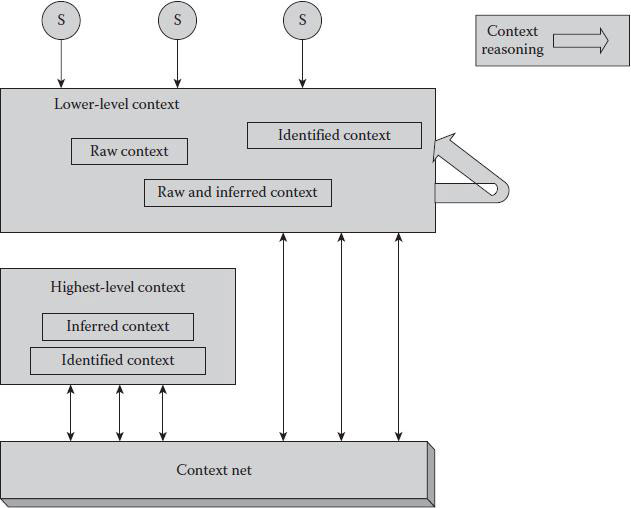
Figure 3.1 Different levels of context.

From the collection point of view, context can be categorized as direct context and indirect context. Direct context refers to gathered information that does not involve any extra processing. If the information is gathered implicitly by means of sensors, it is called sensed context. If the information is gathered explicitly, it is called defined context. Indirect context refers to one inferring information from direct context.

From the application point of view, context falls into low-level context and high-level context. Low-level context information is usually gathered from sensors or from application logs, which can be considered environmental atomic facts. High-level context information is derived from low-level context information.

Finally, context information can be categorized into two categories from a temporal point of view: static context and dynamic context. Static context does not change with time (such as a person’s race). Dynamic context keeps changing in different frequencies depending on the context dimension (such as a person’s location or age). This implies that, for a dynamic context dimension, various values might be available. Hence, management of context information’s temporal character is crucial either in the sense of historical context or in the sense of the validity of available contextual information.

3.1.2  Context Collection Framework

The goal for all context data collection is to capture quality evidence that then translates to rich data analysis and that allows the building of a convincing and credible answer to questions that have been posed. As discussed earlier, context is not simply the state of a fixed set of interaction resources, it is also a process of interacting with an ever-changing environment composed of reconfigurable, migratory, distributed, and multiscale resources. So, dynamic context has to collect during the execution process of pervasive applications, providing context-aware pervasive computing with adaptive capacity for dynamically changing environments. The data collection component of research is common to all fields of study including physical and social sciences, humanities, and business.

WSNs can be used to collect the dynamic context in pervasive systems efficiently due to their flexibility, fault tolerance, high sensing, self-organization, fidelity, low cost, and rapid deployment [3,4]. However, the traditional flat architecture of WSNs, where all sensor nodes send their data to a single sink node by multiple hops, limits large-scale pervasive context collection [5–7].

Figure 3.2 shows an architecture that merges the advantages of mesh networks and WSNs through deploying multiple wireless mesh routers equipped with gateways in each sensor network. It can provide capacities to interconnect multiple homogeneous/heterogeneous sensor networks; to improve the scalability, robustness, and data throughput of sensor networks; and to support the mobility of nodes.

Mesh routers in Figure 3.2 automatically interconnect to form a mesh network while they are connected with the Internet through powerful base stations. In such an architecture, there are three kinds of networks on three logical layers:

■  Wireless sensor network for monitoring objects and reporting the objects’ information (e.g., temperature and humidity)

■  Wireless mesh network for transmitting sensed data long distance and in a reliable way

■  Internet for users to remotely access sensed data

Accordingly, a wireless mesh sensor network (WMSN) is composed of three kinds of nodes: a sensor node, a wireless mesh gateway (WMG), and a wireless mesh router (WMR). In particular, base stations are used to support the mobility of WMGs and WMRs, and they connect the wireless mesh network with the Internet. Sensor nodes continuously or intermittently detect objects and then send data to the most appropriate WMG based on specific routing policies, which will be discussed in detail in the next section. WMGs work as sink nodes and gateways for low-level WSNs as well as routers for middle-level wireless mesh networks. By comparison, WMRs only serve as routers for wireless mesh networks. WMGs and WMRs self-organize as the middle-level wireless mesh network for long-distance transmission and interconnection of sensor networks.

Figure 3.2 A scalable wireless mesh sensor network architecture.

3.2  User Tracking

Location information is one of the most important contexts in pervasive computing [8–10]. With location information, pervasive applications can sense users’ positions and frequent routes, and they can provide location-based, customized service for different users.

In this section, we first discuss technologies for identifying user positions and then we describe a position identification for a mobile robot. Finally, we discuss our experience in managing urban traffic in the city of Shanghai.

3.2.1  Position Identification

Generally speaking, the technologies for locating user position can be categorized into two types, indoor and outdoor techniques. Typically, the outdoor environment uses global positioning system (GPS) sensors for obtaining position information. For an indoor environment, wireless technologies, such as infrared [11], Bluetooth [12,13], and ultrasonic [14,15], have fostered a number of approaches in location sensing. The availability of low-cost, general purpose radio frequency identification (RFID) technology [16–19], has resulted in its being widely used. A typical RFID-based application attaches RFID tags to targeted objects beforehand. Then, either RFID readers or targeted objects move in space. When the tagged objects are within the accessible range of RFID readers, the information stored in the tags is emitted and received by the readers. Thus, the readers know when the objects are within a nearby range.

We have used RFID tags for tracking users’ positions. In particular, we have designed a tag-free activity sensing (TASA) approach using RFID tag arrays for location sensing and route tracking [20]. TASA keeps the monitored objects from attaching RFID tags and is capable of sensing concurrent activity online. TASA deploys passive RFID tags into an array, captures the received signal strength indicator (RSSI) series for all tags all the time, and recovers trajectories by exploring variations in RSSI series. We have also used a similar idea for locating a moving object via readings from RFID tag arrays [16] but using mostly passive tags instead of active tags.

3.2.2  Mobile Robot Position Identification

With technology advancement, home robots are expected to assist humans in a number of different application scenarios. A key capability of these robots is being able to navigate in a known environment in a goal-directed and efficient manner, thereby requiring the robot to determine its own position and orientation.

We have designed a visual position calibration method using colored rectangle signboards for a mobile robot to locate its position and orientation [21]. Figure 3.3 shows our solution for indoor robot navigation. In that environment, the space is divided into many subareas. Between two subareas, there is a relay point in the center of each path. Near each relay point, we set a specially designed signboard for robot position calibration. Every time the robot passes a relay point, the robot will have a chance to calibrate its cumulative position errors. In order to position the signboard in the center of the image, sound beacons were used to control the robot’s head to make it turn directly toward the landmarks [22].

The signboards can use distinguishing colors (e.g., red) so that they can be easily detected from the background, simplifying the region extraction. The rectangular shape is convenient for using the vanishing point method to calculate the relative direction and distance between the robot and the signboards. Using that perspective, two parallel lines projected in a plane surface will intersect at a certain point—called a vanishing point. Vanishing points in a perspective image have been used for reconstructing objects in three-dimensional space with one or more images from different angles [23–25]. The vanishing method can also calculate the relative direction of an object to a perspective point (i.e., the center position of the camera).

Figure 3.3 An environmental map with specially designed signboards for position calibration.

A Canny algorithm is designed to detect the edge of the color area to calculate the vanishing points in the image of the signboard [21]. The advantage of our approach is that it can obtain the relative direction and distance between the signboard and the robot with only a single image. Experimental results showed our method is effective; the errors were between about 1.5 degrees and 3 cm in an array position.

3.2.3  Intelligent Urban Traffic Management

We have developed an intelligent urban traffic management system that not only provides traffic guidance, such as a road status report (free or jammed), but also offers the best path prediction and remaining time estimation. Specifically, from 2006 to 2010, we installed GPS and wireless communication devices on more than 4000 taxis and 2000 buses as a part of the Shanghai Grid project [26]. Each vehicle collects GPS location data and reports the data via a wireless device to a central server. By monitoring a large number of public transportation vehicles, the system performs traffic surveillance and offers traffic information sharing on the Internet.

■  Real-time road status report. The road status denotes the average traffic flux of a road. The bigger the traffic flux is for a road, the more crowded the road is and the slower the traffic moves. From the GPS data of vehicle location and speed information, we compute the average speed of vehicles on a road. As an example, Figure 3.4 shows a snapshot of a real-time traffic condition in Shanghai, where a line represents a road and different colors indicate various traffic conditions: roads colored in black, light gray, and gray denote congestion, light congestion, and normal conditions, respectively. With this application, the traffic information is visualized for the user and is shown in public e-displays. Users can also access the information with Web browsers.

Figure 3.4 Real-time traffic conditions in Shanghai.

■  The best path prediction. The best path refers to a sequence of roads from one place to a specified destination, with a minimal cost dependent on different prediction policies. The best path between two specified places may change from time to time. For example, the best path based on the least time policy is different at different times due to changing road status.

The Best Path Prediction service finds the best path to enable people to travel in Shanghai more conveniently. Currently, this service supports the least time policy and the least fee policy. Figure 3.5 illustrates a recommended route that requires the least time to travel from Huaihai Road to Liyang Road, with a sequence of road names at the top left corner. Users can access this service using Web browsers or mobile phones. For a mobile phone user, the service returns a short message service (SMS) showing a sequence of road names.

■  Remaining time estimation. This application computes the estimated remaining time to a destination (for instance, determining how long before the next bus will arrive at a stop). This kind of question is answered considering real-time traffic information, road and intersection maps, and a vehicle’s position and direction.

Figure 3.5 A recommended route with the shortest travel time.

3.3  Context Reasoning

In pervasive computing, context reasoning enables context awareness for ubiquitous applications. Specifically, context reasoning infers high-level implicit context information from the low-level explicit context information. Existing context reasoning techniques can be classified into two types—exact reasoning and inexact or fuzzy reasoning. In this section, we present an inexact reasoning method, the extended Dempster–Shafer theory for context reasoning (DSCR), in ubiquitous/pervasive computing environments.

Figure 3.6 illustrates our context-aware architecture, which is a hierarchical module consisting of context providers, a manager, and consumers. The context providers gather context data on the environments from sensors. Note that contexts may come from applications and that our context collection is capable of gathering contexts at intervals or on demand. The context manager preprocesses contexts and responds to requests from adaptors and services. After the context information is generated, the context manager will format it, remove inconsistencies in the preprocessing step, and then move into the reasoning step where hidden contexts are derived from present and historical contexts. A historical context database is introduced to store the past contexts because contexts that are updated frequently increase considerably in size. Finally, the context manager notifies adaptors and services and distributes contexts to them according to their specific privacy and security requirements and their resource constraints. Here, we implement a prototype to demonstrate our context-aware architecture. We employ TinyOS 2.0, Micaz, and Microsoft SQL servers to collect, preprocess, and store contexts. Our prototype currently supports devices with Bluetooth, Wi-Fi, and WLAN.

It is noteworthy to point out that DSCR is applied to context collection, reasoning, and storage in the context manager. This enables the context manager to handle imprecise and incomplete contexts.

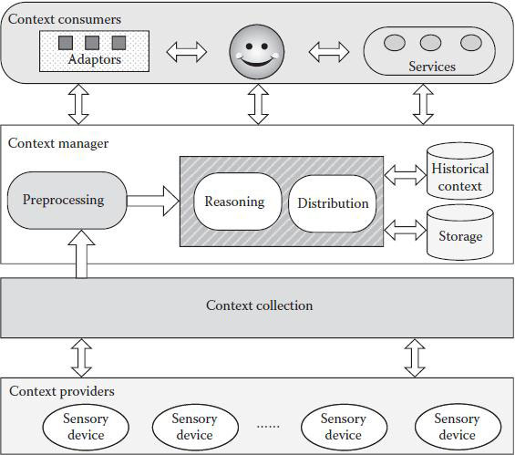
Figure 3.6 The architecture of context-aware pervasive applications. Context providers are responsible for collecting contextual information, which is preprocessed by the context manager in order to derive hidden contexts from present and historical contexts. Finally, the reasoning results are delivered to context consumers.

The rest of this section gives an overview of evidence theory and then discusses our DSCR model in detail. Finally, we discuss the performance of our model in comparison to previous approaches.

3.3.1  Evidence Theory

Evidence theory is a mathematical theory that constructs a coherent picture of reality through computing the probability of an event given evidence [27,28]. Evidence theory is based on the following concepts and principles:

■  Frame of discernment. Let τ be the frame of discernment, denoting a set of mutually exclusive and exhaustive hypotheses about problem domains. The set 2^τ is the power set of τ, denoting the set of all subsets of τ.

■  Mass. Mass stands for a belief mapping from 2^τ to the interval between 0 and 1, represented as m. Let ø and C be the empty set and a subset of τ. The masses of the empty set and the sum of all the subsets in the power set are 0 and 1, respectively. Mass can be assigned to sets or intervals.

■  Belief and plausibility. The belief of a hypothesis is the sum of the beliefs for that hypothesis that are its subsets. Conversely, the plausibility of a hypothesis is the sum of all the beliefs of sets that intersect with it. Belief and plausibility are defined as:

$Bel\left(C\right)={\displaystyle {\displaystyle \sum _{B|B\subseteq C}}m\left(B\right)},Pls\left(C\right)={\displaystyle {\displaystyle \sum _{B|B\cap C\ne \varnothing }}m\left(B\right)}$

(3.1)

where B is a subset of τ. Bel is the degree of belief to which the evidence supports C, constituted by the sum of the masses of all sets enclosed by it. Pls denotes the degree of belief to which the evidence fails to refute C, that is, the degree of belief to which it remains plausible (i.e., the possibility that the hypothesis could happen).

■  Dempster’s rule. In order to aggregate the evidence from multiple sources, Dempster’s rule plays a significantly meaningful and interesting part. Let C_i be a subset of τ and m_j(C_i) be a mass assignment for hypothesis C_i collected from the jth source. For subsets {C₁, C₂, …, C_n} and mass assignments {m₁, m₂, …, m_n}, Dempster’s rule is given as:

$m\left\{C\right\}=\left(m_1\oplus m_2\oplus \dots \oplus m_n\right)\left(C\right)=\frac{1}{K}{\displaystyle {\displaystyle \sum _{\tau =C}}{m}_1\left(C_1\right)m_2\left(C_2\right)\dots m_n\left(C_n\right)}$

(3.2)

where τ equals to C₁ ∩ C₂ ∩ … ∩ C_n, and K is the normalizing constant that is defined as:

$K=1-{\displaystyle {\displaystyle \sum _{\tau =\varnothing }}{m}_1\left(C_1\right)m_2\left(C_2\right)\dots m_n\left(C_n\right)}$

(3.3)

Equations 3.2 and 3.3 show that Dempster’s rule combines evidence over the set of all evidence. Its complexity grows exponentially with increases in the amount of evidence. In Orponen’s study [29], the complexity of Dempster’s rule is proved as NP-complete. Meanwhile, once some probabilities of evidence are zero, Dempster’s rule will get an incorrect inference that a less probable event is regarded as the most probable event that could happen. This phenomenon is called the Zadeh paradox.

3.3.2  DSCR Model

To facilitate understanding of our argument, we present a formal description and a model for DSCR. Let S = {s₁, s₂, …, s_n}, O = {o₁, o₂, …, o_n}, and A = {a₁, a₂, …, a_n} be the sets of sensors, objects, and activities, respectively. Let SO be simple objects monitored by sensors directly, DO be deduced objects obtained from SO, CO be composite objects, E be the set of evidence, and D be the discount rate, reflecting the reliability of sensor readings.

We model DSCR as sensors, objects, and activity layers. Sensors are deployed to monitor objects in the sensors layer. All objects are in the objects layer, where some objects are monitored by sensors. Activity is in the activities layer, which can be inferred according to the contexts of objects. In Figure 3.7, objects o₅ and o₆ are a deduced object and a composite object, respectively, and lines with arrows denote relationships among sensors, objects, and activities. Objects o₁, o₂, o₃, and o₄ are monitored by sensors s₁, s₂, s₃, and s₄, respectively. Object o₅ is deduced from o₁, and o₆ is made up of objects o₂ and o₃. Let us suppose a scenario where a sensor is deployed to monitor the door of a refrigerator where coffee, milk, and tea are stored. When the door is open, users makes drink by selecting coffee, milk, or tea, or their combinations—as simple a₁ or a₂, or complex activity a₃. In this case, the refrigerator is a type of object o₄; coffee, milk, and tea are each a type of object o₅; and their combinations are types of object o₆.

Figure 3.7 DSCR working model.

In Sections 3.3.3, 3.3.4, and 3.3.5, we describe how to apply DSCR to this scenario. The process of applying DSCR consists of (1) propagating evidence in the sensors layer, (2) propagating evidence in the objects layer, and (3) recognizing activity. In Section 3.3.6, we design a computation reduction strategy for DSCR.

3.3.3  Propagating Evidence in the Sensors Layer

Sensors are vulnerable and vary drastically with environments, which leads to unreliable sensor readings. Therefore, it is important to take into account the reliability of sensors in the evidence aggregation process. This reliability is controlled by the sensor discount rate, which is derived from the sensor reliability model [30,31]. In DSCR, the sensor discount rate is incorporated and is defined in Equation 3.4:

$m^r\left(C\right)=\{\begin{array}{ll}\hfill \left(1-r\right)m\left(C\right)& C\ne \text{τ}\hfill \\ \hfill r+\left(1-r\right)m\left(\text{τ}\right)& \text{otherwise}\hfill \end{array}$

(3.4)

where r is the sensor discount rate with its value between 0 and 1. When r is 0, the sensor is completely reliable; when r is 1, the sensor is totally unreliable.

In the beginning, sensors s₁, s₂, s₃, and s₄ are installed and working with discount rates set at 0.02, 0.02, 0.1, and 0.2, respectively. Evidence on sensor nodes is represented by masses as: $m_{s1}\left(s_1\right)=1,m_{s2}\left(s_2\right)=1,m_{s3}\left(\neg s_3\right)=1,\text{and}{m}_{s4}\left(s_4\right)=1$. Then, the discounted masses are calculated as:

$\begin{array}{llllll}\hfill m^r\left(s_1\right)& =\hfill & 0.98;\hfill & \hfill m^r\left(s_1,\neg s_1\right)& =\hfill & 0.98\hfill \\ \hfill m^r\left(s_2\right)& =\hfill & 0.98;\hfill & \hfill m^r\left(s_2,\neg s_2\right)& =\hfill & 0.98\hfill \\ \hfill m^r\left(\neg s_3\right)& =\hfill & 0.9;\hfill & \hfill m^r\left(s_3,\neg s_3\right)& =\hfill & 0.1\hfill \\ \hfill m^r\left(s_4\right)& =\hfill & 0.8;\hfill & \hfill m^r\left(s_4,\neg s_4\right)& =\hfill & 0.2\hfill \end{array}$

There is a relationship between sensors and their associated objects. For example, given the frames τ_a and τ_b of sensor s_a and its associated object o_b, the relationship between sensor s_a and object o_b denotes the evidence propagation from sensors to the objects layer. DSCR associates objects with sensors by maintaining a compatible relationship between them, which is defined as evidential mapping by Equation 3.5:

$\Gamma :m\left(o_b\right)=f\left(s_a\to o_b\right)$

(3.5)

where f is a mapping function, propagating the evidence from sensor s_a to object o_b. For objects o₁, o₂, o₃, and o₄ in Figure 3.7, their masses are computed as:

$\begin{array}{lllll}\Gamma :m\left(o_1\right)\hfill & =\hfill & m^r\left(s_1\right)\hfill & =\hfill & 0.98\hfill \\ \Gamma :m\left(o_1,\neg o_1\right)\hfill & =\hfill & m^r\left(s_1,\neg s_1\right)\hfill & =\hfill & 0.02\hfill \end{array}$

$\begin{array}{lll}\hfill \Gamma :m\left(o_2\right)& =\hfill & m^r\left(s_2\right)=0.98\hfill \\ \hfill \Gamma :m\left(o_2,\neg o_2\right)& =\hfill & m^r\left(s_2,\neg s_2\right)=0.02\hfill \\ \hfill \Gamma :m\left(o_3\right)& =\hfill & m^r\left(s_3\right)=0.9\hfill \\ \hfill \Gamma :m\left(o_3,\neg o_3\right)& =\hfill & m^r\left(s_3,\neg s_3\right)=0.1\hfill \\ \hfill \Gamma :m\left(o_4\right)& =\hfill & m^r\left(s_4\right)=0.8\hfill \\ \hfill \Gamma :m\left(o_4,\neg o_4\right)& =\hfill & m^r\left(s_4,\neg s_4\right)=0.02\hfill \end{array}$

In this step, evidence is propagated to all the sensors and objects. With the help of the mapping function, the masses of sensors are transferred to the objects layer.

3.3.4  Propagating Evidence in the Objects Layer

After the masses of sensors are transferred, this step further propagates the evidence in the objects layer. Suppose we collect evidence from the observations illustrated in Table 3.1. Note that evidence {o₁} → {o₅} refers to a 0.9 confidence about object o₅ when we observe object o₁. We take simple object o₄, deduced object o₅, and composite object o₆ to explain this step.

■  Calculating masses for the deduced objects: DO ← E. Although the deduced objects are not monitored directly by sensors, evidential mapping is capable of calculating their masses from their evidence. For instance, evidential mapping propagates masses from objects o₁ to o₅ as:

$\begin{array}{l}m\left(\left\{o_5\right\}\right)=m\left(\left\{o_1\right\}\right)*m\left(\left\{o_1\right\}\to \left\{o_5\right\}\right)=0.882\\ m\left(\left\{o_5,\neg o_5\right\}\right)=m\left(\left\{o_1\right\}\right)*m\left(\left\{o_1\right\}\to \left\{o_5,\neg o_5\right\}\right)\\ +m\left(\left\{o_1,\neg o_1\right\}\right)*m\left(\left\{o_1,\neg o_1\right\}\to \left\{o_5,\neg o_5\right\}\right)=0.118\end{array}$

Table 3.1 Evidential Mapping

Relationship	Evidence Value
{o1}   → {o5}	0.9
{¬ o1}   → {¬ o5}	1.0
{o1}   → {o5,¬ o5}	0.1
{o1,¬ o1}   → {o5,¬ o5}	1.0
{o4}   → {a2}	0.3
{¬ o4}   → {¬ a2}	1.0
{o4}   → {a2,¬ a2}	0.7
{o4,¬ o4}   → {a2,¬ a2}	1.0

■  Calculating masses for the composite objects: CO ← E. This step aims to propagate the evidence to the composite objects. This is also achieved by evidential mapping and is much more complex than that of the deduced objects. It includes two sub-steps: (1) calculating masses to the sets of objects that comprise the composite objects and (2) calculating masses of the composite objects. In the first sub-step, DSCR computes the masses of these sets using Equation 3.5:

$\begin{array}{lll}\hfill \Gamma :m_1\left(o_2,o_3\right)& =\hfill & m\left(\left\{o_2\right\}\right)=0.98\hfill \\ \hfill \Gamma :m_2\left(o_2,o_3\right)& =\hfill & m\left(\left\{o_3\right\}\right)=0.9\hfill \\ \hfill \Gamma :m_1\left(\left\{o_2,o_3\right\},\neg \left\{o_2,o_3\right\}\right)& =\hfill & m\left(\left\{o_2,\neg o_2\right\}\right)=0.02\hfill \\ \hfill \Gamma :m_2\left(\left\{o_2,o_3\right\},\neg \left\{o_2,o_3\right\}\right)& =\hfill & m\left(\left\{o_3,\neg o_3\right\}\right)=0.1\hfill \end{array}$

Thus, we get different beliefs from two sources (i.e., sensors s₂ and s₃). How to generate the masses of the composite objects is an interesting process. Most existing approaches ignore the difference among the evidence from multiple sources; we use a weighted sum to compute the masses of composite objects, where the weight corresponds to the discount rate for the mass.

■  Generating an activity candidate set from objects: A ← O. So far, we can generate an activity candidate set in which users may undertake one or more activities at a time. Even though knowing precisely what the users want is impossible, observations show that most routine tasks are predictable. In fact, an object–activity mapping table is collected in DSCR that conforms closely to the reality of how users work. This mapping table varies with each scenario, and data can be collected from observations. For instance, in Figure 3.7, activity a₁ obtains the masses propagated by objects o₅ and o₆ according to the object–activity mapping table. Then its mass is calculated as:

$\begin{array}{lll}\hfill m_1\left(\left\{a_1\right\}\right)& =\hfill & m\left(\left\{o_5\right\}\right)=0.882\hfill \\ \hfill m_2\left(\left\{a_1\right\}\right)& =\hfill & m\left(\left\{o_6\right\}\right)=0.948\hfill \\ \hfill m_1\left(\left\{a_1,\neg a_1\right\}\right)& =\hfill & m\left(\left\{o_5,\neg o_5\right\}\right)=0.118\hfill \\ \hfill m_2\left(\left\{a_1,\neg a_1\right\}\right)& =\hfill & m\left(\left\{o_6,\neg o_6\right\}\right)=0.052\hfill \end{array}$

For the same reason, the mass of activity a₂ needs to be calculated. At this point, DSCR has generated an activity candidate set and is ready for user activity recognition in the next step.

3.3.5  Recognizing User Activity

This step focuses on recognizing user activity from the activity candidate set. For example, activity a₁ is chosen because of its bigger mass than that of other activities. Observations in previous steps reveal that the original accuracy of sensors has a significant impact on the final results. Two methods are available to avoid the influence of sensor reliability. One method is to use powerful sensors to improve accuracy, but this increases cost and prevents ubiquitous computing. The other method is to use multiple sensors to monitor the same objects or to sample the same context several times. In most cases, the latter method is preferred for ubiquitous applications because of lower cost.

Table 3.2 Example of an Activity Candidate Set

Activity	m1	m2	m - Final Result
{a1}	0.40	0.20	?
{a2}	0.30	0.20	?
{a3}	0.20	0.30	?
{a1, a2}	0.05	0.15	?
{a2, a3}	0.04	0.10	?
Θ = {a1, a2, a3}	0.01	0.05	?

To clearly describe the mechanism of activity recognition, we extend the example used earlier. Suppose that we collect the evidence for the same scenario and process it by the steps mentioned before (see Table 3.2). According to Equation 3.3, the normalizing constant K is calculated to be 0.477. Then, using Equation 3.2, the combination mass of activity a₁ is computed to be 0.3606.

In the same way, we can calculate the combined masses m{a₂}, m{a₃}, m{a₁, a₂}, m{a₂, a₃}, and m{τ} as 0.3795, 0.2201, 0.0241, 0.0147, and 0.0010, respectively. After all the combination masses have been obtained, applications will compute the beliefs using Equation 3.1 and then will recognize the activity. Correspondingly, activity a₂ in Table 3.2 is selected as the prediction. Up to now, all the steps of applying DSCR into ubiquitous computing environments have been described. However, the problem is still not solved—the intensive computation that arises from calculating the normalizing constant and combined masses [28,29].

3.3.6  Evidence Selection Strategy

In order to solve this problem, we present a strategy—that of evidence selection for Dempster’s rule. The calculation for the normalizing constant K in Dempster’s rule is time-consuming because it requires traversing all the evidence and masses.

We find that the observation illustrated as Lemma 3.1 can reduce the operations for the normalizing constant to |τ|. Note that Dempster’s rule, which uses Equation 3.3 to calculate the normalizing constant, is appropriate for calculating the combined mass for any one hypothesis without calculating all the combined masses.

Lemma 3.1

The normalizing constant K can be computed from all the masses that are to be normalized.

The other computation overhead of DSCR emerges from the calculation of the combined masses. Suppose we calculate the combined mass for evidence C by calculating its unnormalized mass and then normalizing it. The total number of operations required is proportional to log(|C|)+log(|τ|) for ordered lists but is exponential in |τ| for n-dimensional array representation. In view of the fact that the decisions made by ubiquitous applications in most cases rely on the most related contexts, DSCR employs a process of selecting evidence. This process consists of two sub-steps.

First, DSCR defines the importance of evidence by t_i that is given as:

$t_i={\displaystyle {\displaystyle \sum _{j=1}^n}{w}_j*m_j,}$

(3.6)

where j is the number of masses and w_j is the weight of mass m_j for evidence i. Consider that masses from multiple sources have different impacts on the decision making for ubiquitous applications. DSCR is capable of tuning w_j to emphasize the most important masses.

Second, DSCR selects the most related evidence by k−l strategy. Let n be the number of evidence, k be the minimum number of evidence to be kept, l be the maximum number of evidence to be kept, η be the threshold on the sum of masses of selected evidence, Σ be the sum of masses of selected evidence, ϑ be the number of selected evidence, and LSP be the least small probability event. Lines 5 to 17 in Algorithm 3.1 are k−l selection strategy for evidence selection. When l is equal to k, the selection strategy turns into top-K selection strategy. Note that the step of randomized quicksort in k−l strategy is just marking the order of evidence according to the t_i and does not swap evidence orders during the sort process.

For k−l evidence selection strategy, the time complexity is O(n), where n is the amount of evidence. The space complexity is also O(n). For the conflict resolution strategy, the time complexity is O(ϑ), where ϑ is the amount of evidence used in Dempster’s rule. DSCR is scalable even for a large amount of evidence because ϑ is much less than n.

3.3.7  Performance

We compare the performance of DSCR with the typical Bayesian network approach [32–34], D–S theory, and with the Yager [35] and Smets [36] approaches. Note that both rule-based and logic-based approaches are designed for exact reasoning, which cannot work well with imprecise and incomplete context data.

Algorithm 3.1 The Optimized Selection Algorithm

1:  input: e: evidence set

2:  output: et: selected k − l evidence

3:  ai: the prediction result

4:

5:  // k − l selection strategy

6:  // calculate the weighted sum of masses

7:  for i ← 1, n do

8:  compute ti

9:  // rst: result of all ti

10:  rst ←ti

11:  end for

12:

13:  randomized quicksort e based on t

14:  // select top k evidence

15:  et ← e(k)

16:  while (Σ > η && ϑ < l) do

17:  e′ ← the evidence with the next highest mass

18:  end while

Ten user activities are extracted from the MIT Houser_n project, which aimed to facilitate user real life by continuous monitoring and recording all activities of users [37]. The Houser_n project provided the videos, logs, datasets, and nitty-gritty (true activity). In the experiments, we selected singleton and complex activity as test activities, together with associated information, such as their frequency during a sampled month and the surrounding contexts when they happened. Due to a lack of information related to the discount rate of all sensors in the dataset, we assume all sensors work properly with zero discount rate. Finally, we run the experiments nine times with context data from a different month each time.

Figure 3.8 shows the overall performance of DSCR. The x-axis is the i-th experiment. DSCR outperforms the other approaches by about 28.65% in recognition rate. D–S theory achieves a better result than the Bayesian network. This is because the evidence used in these experiments does not contain much highly conflicting evidence. The Yager and Smets approaches alleviate the influence of conflicting evidence and achieve the higher recognition rate. This implies that some evidence is highly conflicting in our test set. Contrary to this, the Bayesian network cannot achieve a high recognition rate.

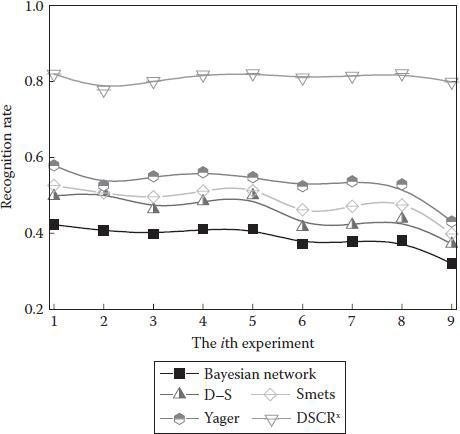
Figure 3.8 Recognition rate of recognition user activity. The higher the recognition rate, the better the performance.

Table 3.2 explains why the Bayesian network fails to handle such evidence. Let α, β, γ, η, ξ, and τ denote six hypotheses a₁, a₂, a₃, {a₁, a₂}, {a₂, a₃} and {a₁, a₂, a₃}, respectively. First, α relates to η and τ, while η, ξ, and τ correlate to each other. They are not exclusive and exhaustive (e.g., {a₁, a₃} is missing). Second, the causal Bayesian network cannot establish the hierarchical relationships among hypotheses when constructing its structure. In fact, hypotheses α, β, and γ are in the same level with η, ξ, and τ. Therefore, the two requirements in the Bayesian network cannot be satisfied, resulting in its failure.

Further Readings

How RFID Works

Kevin Bonsor & Wesley Fenlon “How RFID Works” November 5, 2007. HowStuffWorks.com. http://electronics.howstuffworks.com/gadgets/high-tech-gadgets/rfid.htm, accessed on April 9, 2016.

This article presents the types of RFID tags and discusses how these tags can be used in different cases such as in supply chain and in Departments of State and Homeland Security.

User Tracking

http://people.csail.mit.edu/fadel/wivi/index.html

The site provides information about a new technology named Wi-Vi that use Wi-Fi signals to track moving humans through walls and behind closed doors. Wi-Vi relies on capturing the reflections of its own transmitted signals off moving objects behind a wall in order to track them.

Wireless Sensor Networks

http://www.sensor-networks.org/

This is a site for the Wireless Sensor Networks Research Group, which is made up of research and developer teams throughout all the world that are involved in active projects related to the WSN field. The site provides information about a variety of WSN projects.

Context Data Distribution

P. Bellavista, A. Corradi, M. Fanelli, and L. Foschini, A survey of context data distribution for mobile ubiquitous systems. ACM Comput. Surv. vol. 44, no. 4(24), pp. 1–45, 2012.

This paper analyzes context data distribution that is especially important for context gathering.

Dempster–Shafer Theory

L. Liu and R. R. Yager, Classic works of the dempster-shafer theory of belief functions: an introduction, Studies in Fuzziness and Soft Computing, vol. 219, pp. 1–34, 2008. Springer-Verlag Berlin Heidelberg.

This book brings together a collection of classic research papers on the Dempster–Shafer theory of belief functions.

Context Modelling and Reasoning

C. Bettini, O. Brdiczka, K. Henricksen, J. Indulska, D. Nicklas, A. Ranganathan, and D. Riboni, A Survey of Context Modelling and Reasoning Techniques, Pervasive and Mobile Computing, vol. 6, no. 2, pp. 161–180, 2010.

This paper discusses the requirements for context modeling and reasoning.

References

1.  G. D. Abowd, A. K. Dey, P. J. Brown, N. Davies, M. Smith, and P. Steggles, Towards a Better Understanding of Context and Context-Awareness, in Proceedings of the 1st International Symposium on Handheld and Ubiquitous Computing (HUC’99), 1999, pp. 304–307.

2.  J. W. Kaltz, J. Ziegler, and S. Lohmann, Context-Aware Web Engineering: Modeling and Applications, Revue d’Intelligence Artificielle, vol. 19, no. 3, pp. 439–458, 2005.

3.  M. Yu, A. Malvankar, and W. Su, An Environment Monitoring System Architecture Based on Sensor Networks, International Journal of Intelligent Control and Systems, vol. 10, no. 3, pp. 201–209, 2005.

4.  H. Chao, Y. Q. Chen, and W. Ren, A Study of Grouping Effect on Mobile Actuator Sensor Networks for Distributed Feedback Control of Diffusion Process Using Central Voronoi Tessellations, International Journal of Intelligent Control and Systems, vol. 11, no. 2, pp. 185–190, 2006.

5.   I. F. Akyildiz, W. Su, Y. Sankarasubramaniam, and E. Cayirci, A Survey on Sensor Networks, IEEE Communications Magazine, vol. 40, no. 8, pp. 102–105, 2002.

6.  A. Boukerche, R. Werner Nelem Pazzi, and R. Borges Araujo, Fault-Tolerant Wireless Sensor Network Routing Protocols for the Supervision of Context-Aware Physical Environments, Journal of Parallel and Distributed Computing, vol. 66, no. 4, pp. 586–599, 2006.

7.  K. Akkaya and M. Younis, A Survey on Routing Protocols for Wireless Sensor Networks, Ad Hoc Networks, vol. 3, no. 3. pp. 325–349, 2005.

8.  J. Hightower, and G. Borriello, Location Systems for Ubiquitous Computing, Computer, vol. 34, no. 8, pp. 57–66, 2001.

9.  G. Roussos and V. Kostakos, RFID in Pervasive Computing: State-of-the-Art and Outlook, Pervasive and Mobile Computing, vol. 5, no. 1, pp. 110–131, 2009.

10.  J. Ye, L. Coyle, S. Dobson, and P. Nixon, Ontology-Based Models in Pervasive Computing Systems, The Knowledge Engineering Review, vol. 22, no. 4, pp. 315–347, 2007.

11.  R. Want, A. Hopper, V. Falcão, and J. Gibbons, The active badge location system, ACM Transactions on Information System, vol. 10, pp. 91–102, 1992.

12.  O. Rashid, P. Coulton, and R. Edwards, Providing Location Based Information/Advertising for Existing Mobile Phone Users, Personal and Ubiquitous Computing, vol. 12, no. 1, pp. 3–10, 2008.

13.  U. Bandara, M. Hasegawa, M. Inoue, H. Morikawa, and T. Aoyama, Design and Implementation of a Bluetooth Signal Strength Based Location Sensing System, in Proceedings of the IEEE Radio and Wireless Conference, 2004, pp. 319–322.

14.  A. Harter, A. Hopper, P. Steggles, A. Ward, and P. Webster, The Anatomy of a Context-Aware Application, Wireless Networks, vol. 1, pp. 1–16, 2001.

15.  N. B. Priyantha, A. Chakraborty, and H. Balakrishnan, The Cricket Location-Support System, in Proceedings of the 6th Annual International Conference on Mobile Computing and Networking (MobiCom), 2000, pp. 32–43.

16.  Y. Liu, Y. Zhao, L. Chen, J. Pei, and J. Han, Mining Frequent Trajectory Patterns for Activity Monitoring Using Radio Frequency Tag Arrays, IEEE Transactions on Parallel & Distributed Systems, vol. 23, no. 11, pp. 2138–2149, 2012.

17.  L. M. Ni and A. P. Patil, LANDMARC: Indoor Location Sensing Using Active RFID, in Proceedings of the First IEEE International Conference on Pervasive Computing and Communications, 2003. (PerCom 2003), pp. 407–415, 2003.

18.  C. Qian, H. Ngan, Y. Liu, and L. M. Ni, Cardinality Estimation for Large-Scale RFID Systems, IEEE Transactions on Parallel Distributed Systems, vol. 22, no. 9, pp. 1441–1454, 2011.

19.  P. Wilson, D. Prashanth, and H. Aghajan, Utilizing RFID Signaling Scheme for Localization of Stationary Objects and Speed Estimation of Mobile Objects, in IEEE International Conference on RFID, 2007, pp. 94–99.

20.  D. Zhang, J. Zhou, M. Guo, J. Cao, and T. Li, TASA: Tag-Free Activity Sensing Using RFID Tag Arrays, IEEE Transactions on Parallel Distributed Systems, vol. 22, no. 4, pp. 558–570, 2011.

21.  H. Li, L. Zheng, J. Huang, C. Zhao, and Q. Zhao, Mobile Robot Position Identification with Specially Designed Landmarks, in Fourth International Conference on Frontier of Computer Science and Technology, 2009, pp. 285–291.

22.   H. Li, S. Ishikawa, Q. Zhao, M. Ebana, H. Yamamoto, and J. Huang, Robot navigation and sound based position identification, in IEEE International Conference on Systems, Man and Cybernetics, 2007, pp. 2449–2454.

23.  Y. Liu, T. Yamamura, T. Tanaka, and N. Ohnishi, Extraction and Distortion Rectification of Signboards in a Scene Image for Robot Navigation, Transactions on Electrical and Electronic Engineering Japan C, vol. 120, no. 7, pp. 1026–1034, 2000.

24.  P. Parodi and G. Piccioli, 3D Shape Reconstruction by Using Vanishing Points, IEEE Transactions on Pattern Analysis and Machine Intelligence, vol. 18, no. 2. pp. 211–217, 1996.

25.  R. S. Weiss, H. Nakatani, and E. M. Riseman, An Error Analysis for Surface Orientation from Vanishing Points, IEEE Transactions on Pattern Analysis and Machine Intelligence, vol. 12, no. 12, pp. 1179–1185, 1990.

26.  M. Li, M.-Y. Wu, Y. Li, J. Cao, L. Huang, Q. Deng, X. Lin, et al. ShanghaiGrid: An Information Service Grid, Concurrency and Computation: Practice and Experience, vol. 18, no. 1, pp. 111–135, 2005.

27.  A. P. Dempster, A Generalization of Bayesian Inference, Journal of the Royal Statistical Society Series B, vol. 30, no. 2, pp. 205–247, 1968.

28.  G. Shafer, A Mathematical Theory of Evidence. Princeton University Press, Princeton, New Jersey, 1976.

29.  P. Orponen, Dempster’s Rule of Combination is NP-Complete, Artificial Intelligence, vol. 44, no. 1–2, pp. 245–253, 1990.

30.  S. McClean, B. Scotney, and M. Shapcott, Aggregation of Imprecise and Uncertain Information in Databases, IEEE Transactions on Knowledge and Data Engineering, vol. 13, no. 6, pp. 902–912, 2001.

31.  D. Mercier, B. Quost, and T. Denœux, Refined Modeling of Sensor Reliability in the Belief Function Framework Using Contextual Discounting, Information Fusion, vol. 9, no. 2, pp. 246–258, 2008.

32.  Y. Ma, D. V. Kalashnikov, and S. Mehrotra, Toward Managing Uncertain Spatial Information for Situational Awareness Applications, IEEE Transactions on Knowledge and Data Engineering, vol. 20, no. 10, pp. 1408–1423, 2008.

33.  M. Mamei and R. Nagpal, Macro Programming through Bayesian Networks: Distributed Inference and Anomaly Detection, in Proceedings to the Fifth Annual IEEE International Conference on Pervasive Computing and Communications (PerCom), 2006, pp. 87–93.

34.  A. Ranganathan, J. Al-Muhtadi, and R. H. H. Campbell, Reasoning about Uncertain Contexts in Pervasive Computing Environments, IEEE Pervasive Computing, vol. 3, no. 2, pp. 62–70, 2004.

35.  R. R. Yager, On the Dempster-Shafer Framework and New Combination Rules, Information Sciences (New York), vol. 41, no. 2, pp. 93–137, 1987.

36.  P. Smets, The Combination of Evidence in the Transferable Belief Model, IEEE Transactions Pattern Analysis Machine Intelligence, vol. 12, no. 5, pp. 447–458, 1990.

37.  House_n Project, Department of Architecture, Massachusetts Institute of Technology. [Online]. Available from: http://architecture.mit.edu/house_n/intro.html, accessed on February 15, 2009.