
CHAPTER 2
How to Value a Business
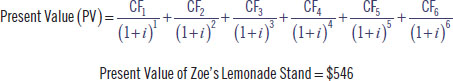
To figure out what Zoe’s Lemonade Stand is worth today (its present value), we need to estimate the cash flows it will generate over its useful life and then discount those cash flows back to the present to account for the time value of money and uncertainty of the cash flow estimates, as we show here
Defining Cash Flow
We first need a definition for the cash flow the business generates. Unfortunately, like many other terms in finance, there is no single definition; rather, there are many. In the interest of simplicity, we defer to Warren Buffett’s definition, which he calls owner earnings, as outlined in the 1986 Berkshire Hathaway Chairman’s Letter:
| Net Income |
| + Depreciation and amortization |
| − Maintenance cap-ex |
| = Owner earnings |
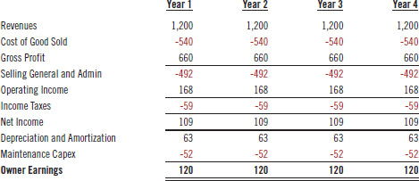
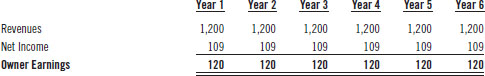
To calculate the net income for Zoe’s Lemonade Stand, we need to build a financial model for her business. This exercise entails forecasting sales, cost of goods sold, SG&A (selling, general, and administrative) expenses, depreciation, and taxes. We must perform this calculation for each year in the forecast period, which in this example is four years, as shown in Table 2.1. To keep the model simple, we will not forecast any growth in revenues in this example.
Table 2.1 Income Statement for Zoe’s Lemonade Stand
How to Calculate Present Value Using a Discounted Cash Flow Model
We use 8.5% as the discount rate (which incorporates both uncertainty and the time value of money) to calculate the present value, or the value in today’s dollars, of Zoe’s Lemonade Stand’s estimated cash flows, as shown in Figure 2.1.
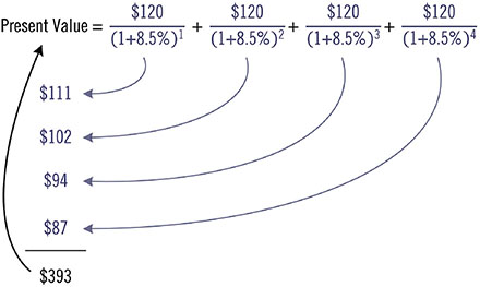
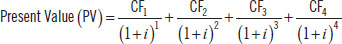

Figure 2.1 Present Value of Four Years of Cash Flows from Zoe’s Lemonade Stand
Although this calculation is relatively straightforward, it raises a couple of obvious questions: Why do we estimate and value only four years of cash flow? Why would the lemonade stand not generate cash flow beyond the four-year forecast period? Unless we are going to operate the business for only four years, it makes sense to include the cash flow from year 5 in the valuation analysis. And the same goes for year 6. We show the calculation with the two additional years included in Figure 2.2.
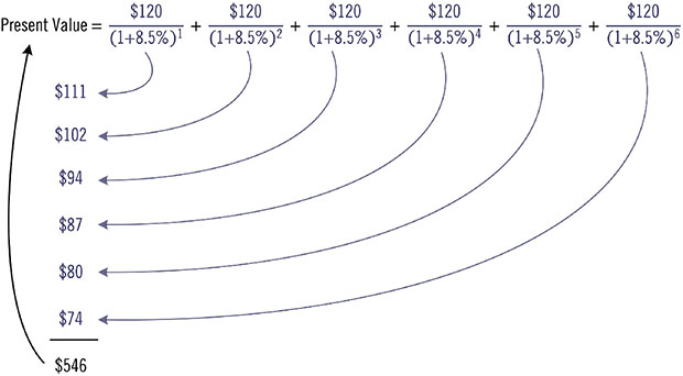
Figure 2.2 Present Value of Six Years of Cash Flows from Zoe’s Lemonade Stand
In fact, it should be apparent that we need to include all of the cash flows the business will generate, over its entire useful life, in the analysis. Therefore, we need to extend the forecast period in the calculation to include all future years, which we designate as year n in the equation shown here:

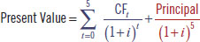
The following formula is the formal way the discounted cash flow (DCF) model is usually presented:
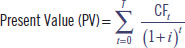
Although more intimidating in this form, the formula merely states that the present value equals the sum of all cash flows the business will generate, over its useful life, discounted back to the current period. It is important to note that the time period in the equation extends from the present until time t, which, in theory, is the end of all time.
While the formula is straightforward, the challenge is estimating the future cash flows to be used as inputs. As we discuss in the previous chapter, there are four subcomponents that we need to consider when estimating future cash flows—timing, duration, magnitude, and growth. Also, it is important to recognize that the formula requires that we estimate cash flows many years into the future. In fact, the formula, in its truest sense, calls for an infinite number of future cash flow estimates.
We also need to consider the time value of money and the level of uncertainty in the cash flow estimates. Unfortunately, the discount rate is not a number one can look up in the newspaper. Although the concept is simple—a dollar today is worth more than a dollar in the future, as we discuss in the prior chapter—the challenge is determining the appropriate discount rate to use.
In practice, most analysts use the interest rate of U.S. government fixed-income securities as a proxy for the time value of money and generally select the rate on a long-dated security, such as a 10-year government note, to match the long duration of the company’s cash flow estimates.
Capturing the uncertainty of future cash flows is more challenging. Less predictable cash flows are less valuable in today’s dollars than are more predictable ones; therefore, we need to discount them at a higher rate. Determining how much higher the discount rate needs to be takes domain-specific knowledge concerning the nature of the business and degree of uncertainty to the future cash flows.
Although using a DCF is the correct way to value future cash flows, the formula is challenging in practice because of the difficulty in estimating all six of the independent components for a time period extended well into the future. Consequentially, few investors use the model in its entirety, with most of them using only an abridged version, which we demonstrate later in the chapter.
Predicting the Future Is Not Easy
Predicting events in the future is difficult and highlights the biggest challenge in using a DCF to value a business. Because the analyst cannot know with certainty what events will transpire, he is forced to make numerous assumptions when predicting future cash flows. For instance, there are a litany of different scenarios that could unfold even with a simple business like Zoe’s Lemonade Stand, each with differing probabilities of occurring, and all resulting in different cash flow predictions.
For example, one future scenario could be that sugar prices increase sharply in a short period of time, without Zoe being able to pass the higher cost on to her customers. As a result, her margins get squeezed (pun intended), which lowers the magnitude of future cash flows. In another scenario, it rains every weekend during the summer, causing lemonade sales to be disappointing because of reduced foot traffic. In yet another scenario, the lemonade stand is damaged in a storm, resulting in higher maintenance expenses to repair the damage. There are an infinite number of such possible scenarios, each with its own probability, making it challenging to predict future cash flows with a high degree of confidence. We show several external factors and their relationship to the four cash flow subcomponents in Figure 2.3.
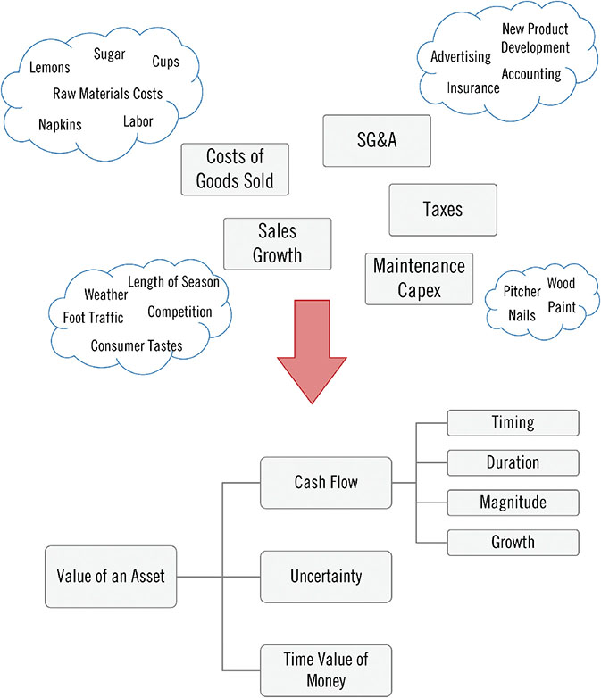
Figure 2.3 External Factors Affecting Cash Flows from Zoe’s Lemonade Stand
Because of the challenges in forecasting future cash flows for even a simple business like a lemonade stand, let alone the significantly greater challenges in forecasting future cash flows for a more complex business, we start with a straight-forward example of valuing a “plain vanilla” bond and then add complexity as we move toward valuing an operating business. The goal is to show how to use a DCF effectively to calculate the value of a business, while recognizing the model’s inherent limitations.
How to Calculate the Present Value of a Bond
We need the following information to value a “plain vanilla” bond using a DCF model:
- Timing—timing of coupon payments and repayment of principal
- Duration—number of payments (time to the bond’s maturity)
- Magnitude—coupon payment amount
- Growth—not applicable since the coupons will not change
- Uncertainty—probability of default (ability to pay)
- Time value of money
Valuing a bond is straightforward because most of the variables are contractually set: the timing of the payments is fixed; duration, which is the number of coupon payments, is fixed; the magnitude, which is the amount of the coupon payment, is fixed; and growth is not applicable since each coupon payment is the same over the life of the bond (in this example). The discount rate used will incorporate the time value of money and capture the uncertainty of the issuing entity’s ability to pay the coupons and repay the principal amount at maturity. We use the following parameters in the example:
- Timing—coupon payments: annual; principal: upon maturity
- Duration—number of payments: five years
- Magnitude—coupon payment rate: 6%
- Growth—not applicable: payments fixed
- Uncertainty—probability of default (ability to pay): low in the example
- Time value of money: 5%2
Because we know each of the components just listed, we can use a five-year DCF to calculate the present value of the cash flows to determine the bond’s value, as shown in Figure 2.4. (NOTE: we will use blue to signify the forecast period and red to signify the principal amount.)
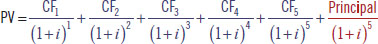
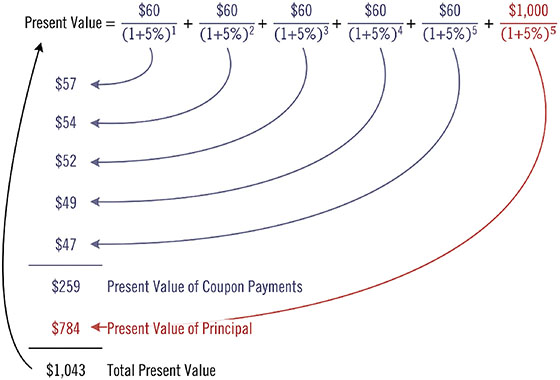
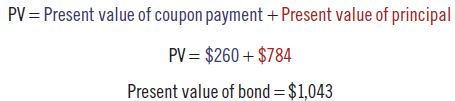
Figure 2.4 Present Value of a “Plain Vanilla” Bond
Or:
The example shows that calculating the present value of a bond is similar to how we calculate the present value of Zoe’s Lemonade Stand in Figure 2.2 above, except the duration is five years instead of six years, and we receive two payments in the final year—the fifth coupon payment and the repayment of the principal amount.
How to Calculate the Present Value of a Perpetuity
Bonds that have no set maturity date are called perpetual bonds, or perpetuities for short. Perpetuities pay regular coupon payments like a bond, except perpetual bonds never mature, as the name implies. As a result, the coupon payments continue forever and the principal is never paid back. Because perpetuities have no maturity date, the duration is infinite. We use the following parameters to value the perpetuity:
- Timing—coupon payments: annual
- Duration—number of payments: infinite
- Magnitude—coupon payment rate: 6%
- Growth—not applicable: payments fixed
- Uncertainty—probability of default (ability to pay): extremely low
- Time value of money: 5%
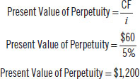
Interestingly, calculating the value of a perpetuity is simpler than the DCF model used to value a standard bond because there is no maturity to the cash flows, as we show with the following formula.
How to Calculate the Present Value of a Business
Valuing a business is similar to valuing a perpetuity because the cash flows the business generates last forever (at least in theory), which matches the duration of the coupon payments from a perpetuity. We will, therefore, use the perpetuity valuation formula as the first step in valuing a business. The main difference between the two entities is that the coupon payments (cash flows) are contractually set with a bond (even with a perpetuity) and are usually the same amount each period. This condition is not the case with a lemonade stand, or any other business, for that matter, because the business’s future cash flows can, and will, vary from year to year—greatly in some cases.
We show the differences in the parameters used in a DCF to value a bond, a perpetuity, and an operating business in Table 2.3.
Table 2.3 Comparison of the Primary Components to the Value of a Bond, Perpetuity, and Zoe’s Lemonade Stand
| "Plain Vanilla" Bond | Perpetuity | Lemonade Stand | |
| Timing: frequency of payments | Annual | Annual | Uncertain |
| Duration: number of payments | 5 years | Infinite | Uncertain |
| Magnitude: coupon payment rate | 6% | 6% | Uncertain |
| Growth | N/A fixed payments | N/A fixed payments | Uncertain |
| Uncertainty: probability of default (ability to pay) | Extremely low | Extremely low | Uncertain |
| Time value of money | 5% | 5% | Uncertain |
While many of the variables in a bond or perpetuity are contractually set, those factors are usually unknown and uncertain in an operating business, as the table shows.
Valuing any asset using the perpetuity formula requires that the cash flows remain constant over time. Although this assumption is unrealistic for an ongoing business, the exercise offers valuable insights and is an important step in ultimately understanding how to value an ongoing operating company. We can use the perpetuity formula to value a business by substituting the coupon payment with the business’s annual cash flows, as we show in the following.
- Where:
- CF = estimated annual cash flow
- i = discount rate
Zoe’s Lemonade Stand generates $120 of cash flow each year, as we show in Table 2.1. The present value of the lemonade stand using the perpetuity formula, with a discount rate of 8.5%, equals $1,412, as shown here:
The calculation captures the six valuation components we discuss in the prior chapter. For instance, because we are using estimated annual cash flows and have set them to be the same each year, the estimates capture timing and magnitude. Also, because we assume the business will generate cash flow every year in the future, the estimates capture duration. And, as with the perpetuity, the discount rate captures the time value of money and uncertainty. What is not captured with this formula is growth, which we discuss in further detail in the next section.
How to Calculate the Present Value of a Growing Cash Flow Stream Using a Two-Stage DCF Model
The valuation process up to this point has been relatively straightforward, mostly because we either knew all the inputs to the DCF model or made simplifying assumptions. And, in all cases, we ignored growth. However, since practically all businesses try to grow over time, growth is an important factor when calculating a company’s present value. Unfortunately, valuing growth is challenging because any formula used to value growth is highly sensitive to the assumptions employed.
A standard method used to value growth is to split the cash flow estimates into multiple stages, which allows the analyst to apply a different growth rate to each stage, and then value each stage separately, with the most common approach using a two-stage model. Using a two-stage model, individual cash flow estimates are made for each year in the first stage, which is called the explicit forecast period, and then each cash flow estimate is discounted back to its present value, as we have done in each example up to this point. The second stage, called the terminal value, captures the value of all cash flows beyond the explicit forecast period, although we then need to discount it back to calculate its present value.
To demonstrate how a two-stage model works, we can use it to value a standard bond. The coupon payments represent the cash flow from the explicit forecast period and the bond’s principal amount represent the terminal value, as we show in Figure 2.5. Not surprisingly, the calculation confirms that we reach the same valuation as when we used the simpler DCF above.
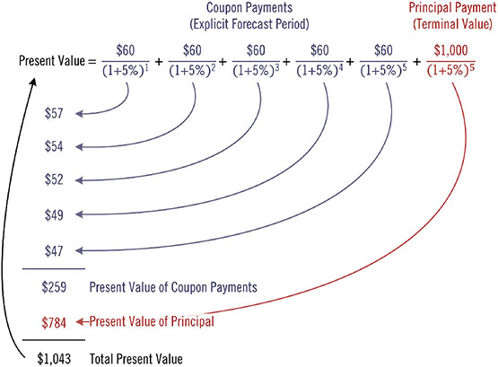
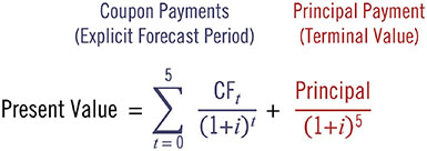
Figure 2.5 Present Value Formula Used to Value a Bond
As we show with the bond valuation in Figure 2.5, it follows that the present value of the present value of the business is the sum of the present value of the cash flows from the explicit forecast period and the present value of the terminal value, as the following equation shows:
The cash flow estimates for the lemonade stand from the explicit forecast period replace the bond’s coupon payments and the lemonade stand’s terminal value replaces the bond’s principal payment. We calculate the present value of the cash flows in the first stage as we have in all the examples and then use the perpetuity formula to represent the lemonade stand’s terminal value as we show in Figure 2.6.
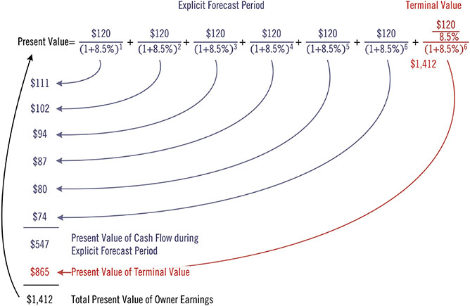
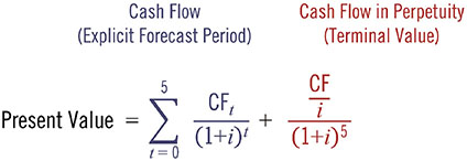
Figure 2.6 Present Value Formula Used to Value a Business
We use a two-stage model to value growth in the next three examples. We vary the growth in the first stage, the explicit forecast period, starting with no growth in the first case, 10% growth in the second case, and 15% growth in the third case. We assume no growth in the terminal value in all three cases.
Two Stage DCF Model with No Growth
The first case assumes no growth during the six-year forecast period, as we show with the explicit cash flow forecasts in Table 2.4.
Table 2.4 Abbreviate Six-Year Forecast of Owner Earnings for Zoe’s Lemonade Stand with No Growth
We can use a DCF model to calculate the present value of the individual cash flows and the terminal value, as demonstrated in Figure 2.7. The calculation shows that the present value of the cash flows from the six-year explicit forecast period totals $547 and the present value of the terminal value equals $865, with the total present value for Zoe’s Lemonade Stand, assuming no growth, totaling $1,412.
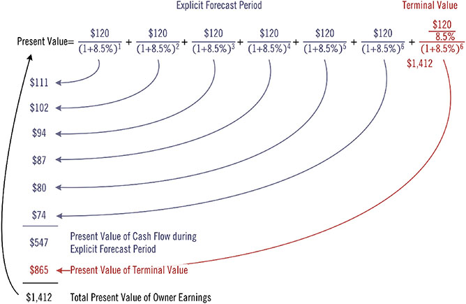
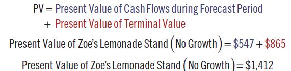
Figure 2.7 Present Value of Zoe’s Lemonade Stand with No Growth
Since the cash flows are constant throughout the company’s life in this example, the value we derive from the two-stage model equals the perpetuity value, as the flowing calculation demonstrates:
Two-Stage DCF Model with 10% Growth
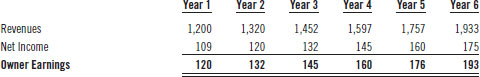
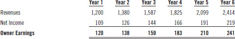
The second case assumes 10% growth in annual cash flow during the explicit forecast period, which we illustrate in Table 2.5, and no growth in perpetuity thereafter.
Table 2.5 Abbreviated Six-Year Forecast of Owner Earnings for Zoe’s Lemonade Stand with 10% Annual Growth
We calculate that the present value of the cash flows from the six-year explicit forecast period equals $687, and the present value of the terminal value equals $1,394. The two values sum to $2,081, which is the total present value of Zoe’s Lemonade Stand in this example, as shown in Figure 2.8.

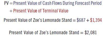
Figure 2.8 Present Value of Zoe’s Lemonade Stand with 10% Annual Growth
Not surprisingly, the present value of the lemonade stand with 10% cash flow growth is higher than the no-growth scenario, as higher growth is more valuable than lower growth, as we outline in Chapter 1.
Two-Stage DCF Model with 15% Growth
The third case assumes 15% growth in annual cash flow during the six-year explicit forecast period, as shown in Table 2.6, and no growth in perpetuity thereafter.
Table 2.6 Abbreviated Six-Year Forecast of Owner Earnings for Zoe’s Lemonade Stand with 15% Annual Growth
We calculate that the present value of the cash flows from the explicit six-year forecast period equals $772 and the present value of the terminal value equals $1,739. The two values sum to $2,511, which is the present value of Zoe’s Lemonade Stand in this example, as shown in Figure 2.9.
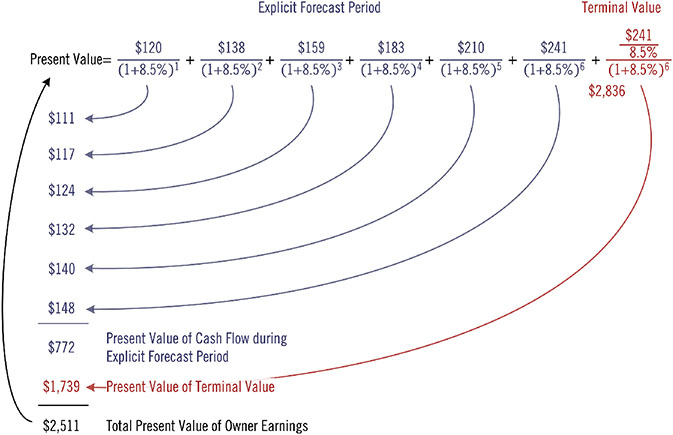
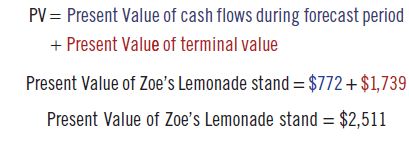
Figure 2.9 Present Value of Zoe’s Lemonade Stand with 15% Annual Growth
The present value of Zoe’s Lemonade Stand with 15% growth is higher than in the two prior examples, which is consistent with the claim that higher growth is more valuable than lower growth, as we discuss in Chapter 1.
How to Think About the Discount Rate
We have used a discount rate of 8.5% in all examples up to this point. We need to address the question, “Is 8.5% the proper discount rate to use?” or what we think is an even better question, “How do we determine what is the appropriate discount rate?”
An in-depth discussion of discount rates is beyond the scope of this book, as academics in finance and investment professionals have published hundreds of books and thousands of journal articles debating the topic. We discuss ways to think about what might be a proper discount rate instead.
Calculating the Cost of Capital
The “correct” rate to use in the discounting process is the company’s cost of capital, which also represents investors’ opportunity cost, making the two returns opposite sides of the same coin. The cost of capital is the rate of return an investor demands to make an investment, while the opportunity cost is the foregone return the investor gives up when he chooses one investment opportunity over another one. A company’s cost of capital has three main components:
- The ratio between debt and equity financing
- The after-tax interest on the company’s borrowings (cost of debt)
- The cost of equity
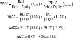
Because the cost of capital is weighted by the ratio of debt to equity, it is called the Weighted Average Cost of Capital, which is known as WACC and calculated using the following formula:
- Where:
- Debt = value of debt
- Equity = market value of equity
- rdebt = cost of debt
- requity = cost of equity
- t = corporate tax rate
Calculating a company’s cost of debt is straightforward, as we show later in the chapter . Calculating a company’s cost of equity, on the other hand, is complicated and requires further explanation. A company’s cost of equity is the return that is required to compensate individuals for investing in the company and is the rate of return investors expect to receive for owning the stock. The return must compensate the individual for the time value of money as well as for the uncertainty of the company’s future financial performance. In other words, the company’s cost of equity is the rate of return necessary to entice investors to purchase the company’s stock.
The Capital Asset Pricing Model3 The basic model used in theoretical finance to calculate a stock’s expected return, and in turn, the company’s cost of equity, is called the capital asset pricing model (CAPM), which was first proposed by William Sharpe and John Litner in the 1960s and is written as follows:
- Where:
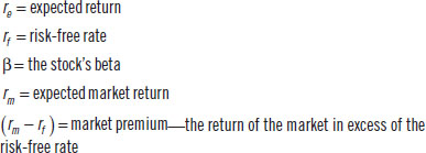
Although a bit intimidating, the CAPM states that the expected return for a security equals the risk-free rate plus a risk premium. The risk-free rate compensates the investor for the time value of money and is customarily represented by the yield on long-term government bonds, such as U.S. Treasuries, while the rest of the equation represents how the investor is compensated for the uncertainty in the business, which requires further explanation.
The Beta Delusion4 A stock’s beta measures its volatility relative to the market and, according to academic finance, represents the stock’s market-related risk. The market premium is the expected market return plus the risk-free rate and is the additional return necessary to compensate investors for holding stocks rather than risk-free assets such as government bonds. The CAPM combines a stock’s beta with the market premium to produce the expected return of the stock given its relative volatility to the market, which is how the capital asset pricing model defines a company’s cost of equity.
Calculating the Weighted Average Cost of Capital for Chemtura
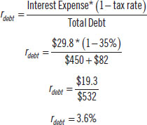
In the following example, we use Chemtura, a specialty chemical company, to show how to calculate a public company’s weighted average cost of capital, using the CAPM. Calculating the company’s cost of debt is relatively easy. At the time of this analysis in 2016, Chemtura had a single bond issue maturing in July 2021 with $450 million outstanding and an interest rate of 5.93%, in addition to a term loan of $82 million, with an interest rate of 3.78%. The cost of debt is calculated after tax6 because interest is tax deductible (all dollar amounts are in millions). Chemtura’s after-tax cost of debt equals 3.6%, as we show in the following calculation:
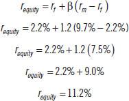
Chemtura’s cost of equity is a bit trickier to calculate. Although there are explicit interest rates with Chemtura’s debt, this is not the case with Chemtura’s equity. We can use the capital asset pricing model to estimate the company’s cost of equity. We selected the 10-year U.S. Treasury Note yielding 2.2% at the time of this writing in May 2016, to represent the risk-free rate; the S&P 500’s long-term historical return of 9.7% for the expected market return; and the number provided on Yahoo! Finance for the stock’s beta.7 We estimate Chemtura’s cost of equity to equal 11.2%, as we show in the following calculation:
We calculate Chemtura’s WACC using the company’s cost of debt of 3.6% and cost of equity of 11.2% (all dollar amounts in billions):
These formulas may seem impressive, particularly in their implied precision, but it is important to note that the only fundamental aspect of the business that is factored into the calculation is Chemtura’s capital structure. The outlook for the business, level of competition, quality of management, and all other fundamental factors are ignored, which is why most professional portfolio managers dismiss using the CAPM to calculate a company’s cost of capital. Although analysts need to understand how companies and investors think about and, in turn, estimate a firm’s weighted average cost of capital, it is important to recognize that the standard approach using CAPM has significant shortcomings.
The Discount Rate Stack
There are numerous factors other than the stock’s relative volatility that should to be considered when determining a company’s cost of capital. These factors are the building blocks of the discount rate stack, which we show in Figure 2.10.
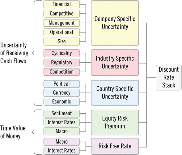
Figure 2.10 Main Factors of the Discount Rate Stack
The discount rate stack is not a formula. It should be viewed more like a checklist of uncertainties that need to be considered when estimating a company’s cost of equity.
When in Doubt, Just Use 10%
Although the cost of capital is vital to every investment decision that an executive must make, calculating a precise cost of equity is probably an impossible task and one that forces investors and business managers alike to settle for an imprecise estimate.
Warren Buffett and Charlie Munger, two of the greatest investors in history, seem to agree with the challenges we outline above, as is reflected in their comments on the topic during the Berkshire Hathaway 2003 annual meeting:
Buffett: Charlie and I don’t know our cost of capital. It’s taught in business schools, but we’re skeptical. We just look to do the most intelligent thing we can with the capital that we have. We measure everything against our alternatives. I’ve never seen a cost of capital calculation that made sense to me. Have you, Charlie?
Munger: Never. If you take the best text in economics by Mankiw, he says intelligent people make decisions based on opportunity costs—in other words, it’s your alternatives that matter. That’s how we make all of our decisions. The rest of the world has gone off on some kick—there’s even a cost of equity capital—perfectly amazing mental malfunction.8
Buffett and Munger acknowledge that calculating a company’s cost of capital, at best, is an inexact art and one that will not result in reaching a precise estimate.
We fear that readers must be asking themselves at this point why we made them suffer through the calculation of Chemtura’s WACC when most professional investors, including Buffett and Munger, feel that beta and the CAPM are inadequate methods for calculating a company’s cost of equity. We presented the example for two reasons. The first was to explain the method taught most often in business schools around the world. The second was to demonstrate that despite the implied precision in the formulas taught, in the end, we calculated Chemtura’s WACC to equal 9.6%, which is essentially the same rate as the S&P’s long-term annual return of 9.7%, and what we believe is an excellent proxy for investors’ long-term opportunity cost.
Professor Bruce Greenwald instructs the students in his value investing class to “Just use 10%. It’s close enough and it makes the math easy.” We agree that it is reasonably safe to use 10% as an estimate for the cost of capital when calculating a company’s value. The analyst can always adjust the rate (up or down) as he gains additional insight into the uncertainties facing the company.
Gems:
- Despite its merits, EBITDA is potentially a poor measure of a company’s true financial performance and can be misleading when used to estimate what a company is worth. Owner earnings is a more accurate metric in both situations.
- Although a DCF is the economically correct way to value future cash flows, the formula is challenging to use in practice because of the difficulty in estimating all six of the independent components for a period of time extended well into the future. Consequentially, few investors use the model in its entirety, with most using an abridged version.
- Despite what portfolio managers claim is their preferred valuation method—enterprise value to EBITDA multiple, P/E ratio, price to sales, caprate, private market value, sum of parts, or liquidation value—they are performing, at the core, a discounted cash flow analysis, either explicitly or implicitly, whether they believe it or not.
- Calculating a company’s cost of debt is straightforward. Calculating a company’s cost of equity, on the other hand, is complicated. A company’s cost of equity is the return required to compensate individuals for investing in the company and is the rate of return investors expect to receive from owning the stock. The return must compensate the individual for the time value of money as well as the uncertainty of the company’s future financial performance. In other words, the company’s cost of equity is the rate of return necessary to entice investors to purchase the company’s stock.
- Professional investors rarely view a stock’s volatility as the primary fundamental risk of investing in a company and, in turn, dismiss the relevancy of beta and CAPM to investing because the methodology ignores important fundamentals of the business.
- Although the cost of capital is vital to every investment decision that an executive must make, calculating a precise cost of equity is probably an impossible goal and one that forces investors and business managers alike to settle for an imprecise estimate.
- At the end of the day, heed the words of Columbia Business School Professor Bruce Greenwald, “Just use 10%. It’s close enough and it makes the math easy.”