
Introducing Gumboot
Gumboot is a fast bootloader and full read/write RWTS. It fits in four sectors on track 0, including a boot sector. It uses only six pages of memory for all its code, data, and scratch space. It uses no zero page addresses after boot. It can start the game from a cold boot in three seconds. That’s twice as fast as the original disk.
qkumba wrote it from scratch, because of course he did. I, um, mostly just cheered.
After boot-time initialization, Gumboot is dead simple and always ready to use:
entry |
command |
parameters |
$BD00 |
read |
A = first track Y = first page X = sector count |
$BE00 |
write |
A = sector Y = page |
$BF00 |
seek |
A = track |
That’s it. It’s so small, there’s $80 unused bytes at $BF80. You could fit a cute message in there! (We didn’t.)
Some important notes:
(1) The read routine reads consecutive tracks in physical sector order into consecutive pages in memory. There is no translation from physical to logical sectors.
(2) The write routine writes one sector, and also assumes a physical sector number.
(3) The seek routine can seek forward or back to any whole track. I mention this because some fastloaders can only seek forward.
I said Gumboot takes six pages in memory, but I’ve only mentioned three. The other three are for data:
$BA00..$BB55 is scratch space for write. Technically this is available so long as you don’t mind them being clobbered during disk write.

$BB00..$BCFF is filled with data tables which are initialized once during boot.
Gumboot Boot0
Gumboot starts, as all disks start, on track $00. Sector $00 (boot0) reuses the disk controller ROM routine to read sector $0E, $0D, and $0C (boot1). Boot0 creates a few data tables, modifies the boot1 code to accommodate booting from any slot, and jumps to it.
Boot0 is loaded at $0800 by the disk controller ROM routine.
0800 [01] Tell the ROM to load only this sector. We’ll
do the rest manually.
0801 4A LSR The accumulator is #$01 after loading sector
$00, #$03 after loading sector $0E, #$05 after
loading sector $0D, and #$07 after loading
sector $0C. We shift it right to divide by 2,
then use that to calculate the load address of
the next sector.
0802 69 BC ADC #$BC Sector $0E → $BD00
Sector $0D → $BE00
Sector $0C → $BF00
0804 85 27 STA $27 Store the load address.
0806 0A ASL Shift the accumulator again now that we’ve
0807 0A ASL stored the load address.
0808 8A TXA Transfer X (boot slot x16) to the accumulator,
which will be useful later but doesn’t affect
the carry flag we may have just tripped with
the two ASL instructions.
0809 B0 0D BCS $0818 If the two ASL instructions set the carry flag, it
means the load address was at least #$C0,
which means we’ve loaded all the sectors we
wanted to load and we should exit this loop.
080B E6 3D INC $3D Set up next sector number to read. The disk
controller ROM does this once already, but
due to quirks of timing, it’s much faster to
increment it twice so the next sector you want
to load is actually the next sector under the
drive head. Otherwise you end up waiting for
the disk to spin an entire revolution, which is
quite slow.
080D 4A LSR Set up the return address to jump to the read
080E 4A LSR sector entry point of the disk controller ROM.
080F 4A LSR This could be anywhere in $Cx00 depending on
0810 4A LSR the slot we booted from, which is why we put
0811 09 C0 ORA #$C0 the boot slot in the accumulator at $0808.
0813 48 PHA Push the entry point on the stack.
0814 A9 5B LDA #$5B
0816 48 PHA
0817 60 RTS Return to the entry point via RTS. The disk
controller ROM always jumps to $0801
(remember, that’s why we had to move it and
patch it to trace the boot all the way back on
page 200), so this entire thing is a loop that
only exits via the BCS branch at $0809.
0818 09 8C ORA #$8C Execution continues here (from $0809) after
081A A2 00 LDX #$00 three sectors have been loaded into memory at
081C BC AF 08 LDY $08AF,X $BD00..$BFFF. There are a number of places in
081F 84 26 STY $26 boot1 that hit a slot-specific soft switch (read
0821 BC B0 08 LDY $08B0,X a nibble from disk, turn off the drive, &c.).
0824 F0 0A BEQ $0830 Rather than the usual form of LDA $C08C,X, we
0826 84 27 STY $27 will use LDA $C0EC and modify the $EC byte in
0828 A0 00 LDY #$00 advance, based on the boot slot. $08A4 is an
082A 91 26 STA ($26),Y array of all the places in the Gumboot code
082C E8 INX that get this adjustment.
082D E8 INX
082E D0 EC BNE $081C
0830 29 F8 AND #$F8 Munge $EC → $E8, used later to turn off the
0832 8D FC BD STA $BDFC drive motor.
0835 09 01 ORA #$01 Munge $E8 → $E9, used later to turn on the
0837 8D 0B BD STA $BD0B drive motor.
083A 8D 07 BE STA $BE07
083D 49 09 EOR #$09 Munge $E9 → $E0, used later to move the drive
083F 8D 54 BF STA $BF54 head via the stepper motor.
0842 29 70 AND #$70 Munge $E0 → $60 (boot slot x16), used during
0844 8D 37 BE STA $BE37 seek and write routines.
0847 8D 69 BE STA $BE69
084A 8D 7F BE STA $BE7F
084D 8D AC BE STA $BEAC
6 + 2
Before I dive into the next chunk of code, I get to pause and explain a little bit of theory. As you probably know if you’re the sort of person who’s read this far already, Apple ][ floppy disks do not contain the actual data that ends up being loaded into memory. Due to hardware limitations of the original Disk II drive, data on disk is stored in an intermediate format called “nibbles.” Bytes in memory are encoded into nibbles before writing to disk, and nibbles that you read from the disk must be decoded back into bytes. The round trip is lossless but requires some bit wrangling.
Decoding nibbles-on-disk into bytes-in-memory is a multi-step process. In “6-and-2 encoding” (used by DOS 3.3, ProDOS, and all “.dsk” image files), there are 64 possible values that you may find in the data field. (In the range $96..$FF, but not all of those, because some of them have bit patterns that trip up the drive firmware.) We’ll call these “raw nibbles.”
Step 1) read $156 raw nibbles from the data field. These values will range from $96 to $FF, but as mentioned earlier, not all values in that range will appear on disk.
Now we have $156 raw nibbles.
Step 2) decode each of the raw nibbles into a 6-bit byte between 0 and 63. (%00000000 and %00111111 in binary.) $96 is the lowest valid raw nibble, so it gets decoded to 0. $97 is the next valid raw nibble, so it’s decoded to 1. $98 and $99 are invalid, so we skip them, and $9A gets decoded to 2. And so on, up to $FF (the highest valid raw nibble), which gets decoded to 63.
Now we have $156 6-bit bytes.
Step 3) split up each of the first $56 6-bit bytes into pairs of bits. In other words, each 6-bit byte becomes three 2-bit bytes. These 2-bit bytes are merged with the next $100 6-bit bytes to create $100 8-bit bytes. Hence the name, “6-and-2” encoding.
The exact process of how the bits are split and merged is… complicated. The first $56 6-bit bytes get split up into 2-bit bytes, but those two bits get swapped such that %01 becomes %10 and vice-versa. The other $100 6-bit bytes each get multiplied by four. (Bit-shifted two places left.) This leaves a hole in the lower two bits, which is filled by one of the 2-bit bytes from the first group.
The diagram on page 272 might help. “a” through “x” each represent one bit.
Tada! Four 6-bit bytes
00abcdef
00ghijkl
00mnopqr
00stuvwx
become three 8-bit bytes
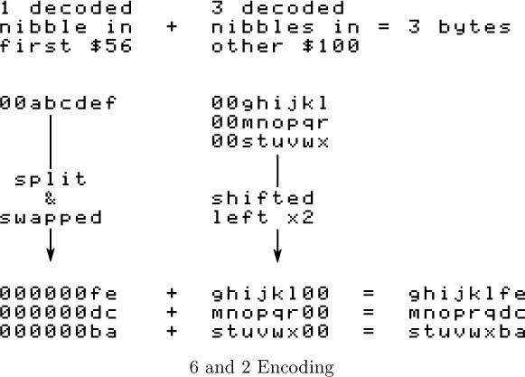
ghijklfe
mnoprqdc
stuvwxba
When DOS 3.3 reads a sector, it reads the first $56 raw nibbles, decoded them into 6-bit bytes, and stashes them in a temporary buffer at $BC00. Then it reads the other $100 raw nibbles, decodes them into 6-bit bytes, and puts them in another temporary buffer at $BB00. Only then does DOS 3.3 start combining the bits from each group to create the full 8-bit bytes that will end up in the target page in memory. This is why DOS 3.3 “misses” sectors when it’s reading, because it’s busy twiddling bits while the disk is still spinning.
Gumboot also uses “6-and-2” encoding. The first $56 nibbles in the data field are still split into pairs of bits that will be merged with nibbles that won’t come until later. But instead of waiting for all $156 raw nibbles to be read from disk, it interleaves the nibble reads with the bit twiddling required to merge the first $56 6-bit bytes and the $100 that follow. By the time Gumboot gets to the data field checksum, it has already stored all $100 8-bit bytes in their final resting place in memory. This means that we can read all 16 sectors on a track in one revolution of the disk. That’s what makes it crazy fast.
To make it possible to twiddle the bits and not miss nibbles as the disk spins,3 we do some of the work in advance. We multiply each of the 64 possible decoded values by 4 and store those values (Since this is done by bit shifting and we’re doing it before we start reading the disk, this is called the “pre-shift” table.) We also store all possible 2-bit values in a repeating pattern that will make it easy to look them up later. Then, as we’re reading from disk (and timing is tight), we can simulate bit math with a series of table lookups. There is just enough time to convert each raw nibble into its final 8-bit byte before reading the next nibble.
The first table, at $BC00..$BCFF, is three columns wide and 64 rows deep. Noting that 3 × 64 is not 256, only three of the columns are used; the fourth (unused) column exists because multiplying by 3 is hard but multiplying by 4 is easy in base 2. The three columns correspond to the three pairs of 2-bit values in those first $56 6-bit bytes. Since the values are only 2 bits wide, each column holds one of four different values. (%00, %01, %10, or %11.)
The second table, at $BB96..$BBFF, is the “pre-shift” table. This contains all the possible 6-bit bytes, in order, each multiplied by 4. (They are shifted to the left two places, so the 6 bits that started in columns 0-5 are now in columns 2-7, and columns 0 and 1 are zeroes.) Like this:
00ghijkl -> ghijkl00
Astute readers will notice that there are only 64 possible 6-bit bytes, but this second table is larger than 64 bytes. To make lookups easier, the table has empty slots for each of the invalid raw nibbles. In other words, we don’t do any math to decode raw nibbles into 6-bit bytes; we just look them up in this table (offset by $96, since that’s the lowest valid raw nibble) and get the required bit shifting for free.
addr |
raw |
decoded 6-bit |
pre-shift |
$BB96 |
$96 |
0 = %00000000 |
%00000000 |
$BB97 |
$97 |
1 = %00000001 |
%00000100 |
$BB98 |
$98 |
[invalid raw nibble] |
|
$BB99 |
$99 |
[invalid raw nibble] |
|
$BB9A |
$9A |
2 = %00000010 |
%00001000 |
$BB9B |
$9B |
3 = %00000011 |
%00001100 |
$BB9C |
$9C |
[invalid raw nibble] |
|
$BB9D |
$9D |
4 = %00000100 |
%00010000 |
. |
|||
. |
|||
. |
|||
$BBFE |
$FE |
62 = %00111110 |
%11111000 |
$BBFF |
$FF |
63 = %00111111 |
%11111100 |
Each value in this “pre-shift” table also serves as an index into the first table with all the 2-bit bytes. This wasn’t an accident; I mean, that sort of magic doesn’t just happen. But the table of 2-bit bytes is arranged in such a way that we can take one of the raw nibbles to be decoded and split apart (from the first $56 raw nibbles in the data field), use each raw nibble as an index into the pre-shift table, then use that pre-shifted value as an index into the first table to get the 2-bit value we need.
Back to Gumboot
This is the loop that creates the pre-shift table at $BB96. As a special bonus, it also creates the inverse table that is used during disk write operations, converting in the other direction.
0850 A2 3F LDX #$3F 0865 B0 10 BCS $0877
0852 86 FF STX $FF 0867 4A LSR
0854 E8 INX 0868 D0 FB BNE $0865
0855 A0 7F LDY #$7F 086A CA DEX
0857 84 FE STY $FE 086B 8A TXA
0859 98 TYA 086C 0A ASL
085A 0A ASL 086D 0A ASL
085B 24 FE BIT $FE 086E 99 80 BB STA $BB80,Y
085D F0 18 BEQ $0877 0871 98 TYA
085F 05 FE ORA $FE 0872 09 80 ORA #$80
0861 49 FF EOR #$FF 0874 9D 56 BB STA $BB56,X
0863 29 7E AND #$7E 0877 88 DEY
0878 D0 DD BNE $0857
And this is the result, where “..” means that the address is uninitialized and unused.
BB90 00 04 BBC8 .. .. .. 6C .. 70 74 78
BB98 .. .. 08 0C .. 10 14 18 BBD0 .. .. .. 7C .. .. 80 84
BBA0 .. .. .. .. .. .. 1C 20 BBD8 .. 88 8C 90 94 98 9C A0
BBA8 .. .. .. 24 28 2C 30 34 BBE0 .. .. .. .. .. A4 A8 AC
BBB0 .. .. 38 3C 40 44 48 4C BBE8 .. B0 B4 B8 BC C0 C4 C8
BBB8 .. 50 54 58 5C 60 64 68 BBF0 .. .. CC D0 D4 D8 DC E0
BBC0 .. .. .. .. .. .. .. .. BBF8 .. E4 E8 EC F0 F4 F8 FC
Next up: a loop to create the table of 2-bit values at $BC00, magically arranged to enable easy lookups later.
087A 84 FD STY $FD 0890 29 03 AND #$03
087C 46 FF LSR $FF 0892 AA TAX
087E 46 FF LSR $FF 0893 C8 INY
0880 BD BD 08 LDA $08BD,X 0894 C8 INY
0883 99 00 BC STA $BC00,Y 0895 C8 INY
0886 E6 FD INC $FD 0896 C8 INY
0888 A5 FD LDA $FD 0897 C0 03 CPY #$03
088A 25 FF AND $FF 0899 B0 E5 BCS $0880
088C D0 05 BNE $0893 089B C8 INY
088E E8 INX 089C C0 03 CPY #$03
088F 8A TXA 089E 90 DC BCC $087C
This is the result:
BC00 00 00 00 .. 00 00 02 .. BC80 01 00 00 .. 01 00 02 ..
BC08 00 00 01 .. 00 00 03 .. BC88 01 00 01 .. 01 00 03 ..
BC10 00 02 00 .. 00 02 02 .. BC90 01 02 00 .. 01 02 02 ..
BC18 00 02 01 .. 00 02 03 .. BC98 01 02 01 .. 01 02 03 ..
BC20 00 01 00 .. 00 01 02 .. BCA0 01 01 00 .. 01 01 02 ..
BC28 00 01 01 .. 00 01 03 .. BCA8 01 01 01 .. 01 01 03 ..
BC30 00 03 00 .. 00 03 02 .. BCB0 01 03 00 .. 01 03 02 ..
BC38 00 03 01 .. 00 03 03 .. BCB8 01 03 01 .. 01 03 03 ..
BC40 02 00 00 .. 02 00 02 .. BCC0 03 00 00 .. 03 00 02 ..
BC48 02 00 01 .. 02 00 03 .. BCC8 03 00 01 .. 03 00 03 ..
BC50 02 02 00 .. 02 02 02 .. BCD0 03 02 00 .. 03 02 02 ..
BC58 02 02 01 .. 02 02 03 .. BCD8 03 02 01 .. 03 02 03 ..
BC60 02 01 00 .. 02 01 02 .. BCE0 03 01 00 .. 03 01 02 ..
BC68 02 01 01 .. 02 01 03 .. BCE8 03 01 01 .. 03 01 03 ..
BC70 02 03 00 .. 02 03 02 .. BCF0 03 03 00 .. 03 03 02 ..
BC78 02 03 01 .. 02 03 03 .. BCF8 03 03 01 .. 03 03 03 ..
And with that, Gumboot is fully armed and operational.
08A0 A9 B2 LDA #$B2 Push a return address on the stack. We’ll come
08A2 48 PHA back to this later. (Ha ha, get it, come back to
08A3 A9 F0 LDA #$F0 it? OK, let’s pretend that never happened.)
08A5 48 PHA
08A6 A9 01 LDA #$01 Set up an initial read of three sectors from
08A8 A2 03 LDX #$03 track 1 into $B000 .. $B2FF . This contains the
08AA A0 B0 LDY #$B0 high scores data, zero page, and a new output
vector that interfaces with Gumboot.
08AC 4C 00 BD JMP $BD00 Read all that from disk and exit via the return
address we just pushed on the stack at $0895.
Execution will continue at $B2F1, once we read that from disk. $B2F1 is new code I wrote, and I promise to show it to you. But first, I get to finish showing you how the disk read routine works.
Read & Go Seek
In a standard DOS 3.3 RWTS, the softswitch to read the data latch is LDA $C08C,X, where X is the boot slot times 16, to allow disks to boot from any slot. Gumboot also supports booting and reading from any slot, but instead of using an index, most fetch instructions are set up in advance based on the boot slot. Not only does this free up the X register, it lets us juggle all the registers and put the raw nibble value in whichever one is convenient at the time (We take full advantage of this freedom.) I’ve marked each pre-set softswitch with ![]() .
.
There are several other instances of addresses and constants that get modified while Gumboot is executing. I’ve left these with a bogus value $D1 and marked them with ![]() .
.
Gumboot’s source code should be available from the same place you found this write-up. If you’re looking to modify this code for your own purposes, I suggest you “use the source, Luke.”
*BD00L
BD00 0A ASL A is the track number to seek to. We multiply
BD01 8D 10 BF STA $BF10 it by two to convert it to a phase, then store it
inside the seek routine which we will call
shortly.
BD04 8E EF BD STX $BDEF X is the number of sectors to read.
BD07 8C 24 BD STY $BD24 Y is the starting address in memory.
BD0A AD E9 C0 LDA $C0E9 ![]() Turn on the drive motor.
Turn on the drive motor.
BD0D 20 75 BF JSR $BF75 Poll for real nibbles (#$FF followed by
non-#$FF) as a way to ensure the drive has
spun up fully.
BD10 A9 10 LDA #$10 Are we reading this entire track?
BD12 CD EF BD CMP $BDEF
BD15 B0 01 BCS $BD18 yes -> branch
BD17 AA TAX no
BD18 8E 94 BF STX $BF94
BD1B 20 04 BF JSR $BF04 seek to the track we want
BD1E AE 94 BF LDX $BF94 Initialize an array of which sectors we’ve read
BD21 A0 00 LDY #$00 from the current track. The array is in
BD23 A9 D1 LDA #$D1 ![]() physical sector order, thus the RWTS assumes
physical sector order, thus the RWTS assumes
BD25 99 84 BF STA $BF84,Y data is stored in physical sector order on each
BD28 EE 24 BD INC $BD24 track. (This saves 18 bytes: 16 for the table
BD2B C8 INY and two for the lookup command!) Values are
BD2C CA DEX the actual pages in memory where that sector
BD2D D0 F4 BNE $BD23 should go, and they get zeroed once the sector
is read, so we don’t waste time decoding the
BD2F 20 D5 BE JSR $BED5 same sector twice.
*BED5L
BED5 20 E4 BE JSR $BEE4 This routine reads nibbles from disk until it
BED8 C9 D5 CMP #$D5 finds the sequence D5 AA, then it reads one
BEDA D0 F9 BNE $BED5 more nibble and returns it in the accumulator.
BEDC 20 E4 BE JSR $BEE4 We reuse this routine to find both the address
BEDF C9 AA CMP #$AA and data field prologues.
BEE1 D0 F5 BNE $BED8
BEE3 A8 TAY
BEE4 AD EC C0 LDA $C0EC ![]()
BEE7 10 FB BPL $BEE4
BEE9 60 RTS
Continuing from $BD32…
BD32 49 AD EOR #$AD If that third nibble is not #$AD, we assume
BD34 F0 35 BEQ $BD6B it’s the end of the address prologue (#$96
would be the third nibble of a standard
BD36 20 C2 BE JSR $BEC2 address prologue, but we don’t actually
check.) We fall through and start decoding the
*BEC2L 4-4 encoded values in the address field.
BEC2 A0 03 LDY #$03 This routine parses the 4-4 encoded values in
BEC4 20 E4 BE JSR $BEE4 the address field. The first time through this
BEC7 2A ROL loop, we’ll read the disk volume number. The
BEC8 8D E0 BD STA $BDE0 second time, we’ll read the track number. The
BECB 20 E4 BE JSR $BEE4 third time, we’ll read the physical sector
BECE 2D E0 BD AND $BDE0 number. We don’t actually care about the disk
BED1 88 DEY volume or the track number, and once we get
BED2 D0 F0 BNE $BEC4 the sector number, we don’t verify the address
field checksum.
BED4 60 RTS On exit, the accumulator contains the physical
sector number.
Continuing from $BD39:
BD39 A8 TAY Use the physical sector number as an index
into the sector address array.
BD3A BE 84 BF LDX $BF84,Y Get the target page, where we want to store
this sector in memory.
BD3D F0 F0 BEQ $BD2F If the target page is #$00, it means we’ve
already read this sector, so loop back to find
the next address prologue.
BD3F 8D E0 BD STA $BDE0 Store the physical sector number later in this
routine.
BD42 8E 64 BD STX $BD64 Store the target page in several places
BD45 8E C4 BD STX $BDC4 throughout this routine.
BD48 8E 7C BD STX $BD7C
BD4B 8E 8E BD STX $BD8E
BD4E 8E A6 BD STX $BDA6
BD51 8E BE BD STX $BDBE
BD54 E8 INX
BD55 8E D9 BD STX $BDD9
BD58 CA DEX
BD59 CA DEX
BD5A 8E 94 BD STX $BD94
BD5D 8E AC BD STX $BDAC
BD60 A0 FE LDY #$FE Save the two bytes immediately after the
BD62 B9 02 D1 LDA $D102,Y target page, because we’re going to use them
BD65 48 PHA for temporary storage We’ll restore them later.
BD66 C8 INY
BD67 D0 F9 BNE $BD62
BD69 B0 C4 BCS $BD2F This is an unconditional branch.
BD6B E0 00 CPX #$00 Execution continues here from $BD34 after
matching the data prologue.
BD6D F0 C0 BEQ $BD2F If X is still #$00, it means we found a data
prologue before we found an address prologue.
In that case, we have to skip this sector,
because we don’t know which sector it is and
we wouldn’t know where to put it. Sad!
Nibble loop #1 reads nibbles $00..$55, looks up the corresponding offset in the preshift table at $BB96, and stores that offset in the temporary two-byte buffer after the target page.
BD6F 8D 7E BD STA $BD7E Initialize rolling checksum to #$00, or update
it with the results from the calculations below.
BD72 AE EC C0 LDX $C0EC![]() Read one nibble from disk.
Read one nibble from disk.
BD75 10 FB BPL $BD72
BD77 BD 00 BB LDA $BB00,X The nibble value is in the X register now. The
lowest possible nibble value is $96 and the
highest is $FF. To look up the offset in the
table at $BB96 , we index off $BB00 + X. Math!
BD7A 99 02 D1 STA $D102,Y Now the accumulator has the offset into the
![]() table of individual 2-bit combinations
table of individual 2-bit combinations
($BC00 .. $BCFF ). Store that offset in a temporary
buffer towards the end of the target page. (It
will eventually get overwritten by full 8-bit
bytes, but in the meantime it’s a useful
$56-byte scratch space.)
BD7D 49 D1 EOR #$D1 ![]() The EOR value is set at $BD6F each time
The EOR value is set at $BD6F each time
through loop #1.
BD7F C8 INY The Y register started at #$AA (set by the TAY
BD80 D0 ED BNE $BD6F instruction at $BD39), so this loop reads a total
of #$56 nibbles.
Here endeth nibble loop #1.
Nibble loop #2 reads nibbles $56..$AB, combines them with bits 0-1 of the appropriate nibble from the first $56, and stores them in bytes $00..$55 of the target page in memory.
BD82 A0 AA LDY #$AA
BD84 AE EC C0 LDX $C0EC ![]()
BD87 10 FB BPL $BD84
BD89 5D 00 BB EOR $BB00,X
BD8C BE 02 D1 LDX $D102,Y
![]()
BD8F 5D 02 BC EOR $BC02,X
BD92 99 56 D1 STA $D156,Y This address was set at $BD5A based on the
![]() target page (minus 1 so we can add Y from
target page (minus 1 so we can add Y from
BD95 C8 INY #$AA..#$FF).
BD96 D0 EC BNE $BD84
Here endeth nibble loop #2.
Nibble loop #3 reads nibbles $AC..$101, combines them with bits 2-3 of the appropriate nibble from the first $56, and stores them in bytes $56..$AB of the target page in memory.
BD98 29 FC AND #$FC
BD9A A0 AA LDY #$AA
BD9C AE EC C0 LDX $C0EC ![]()
BD9F 10 FB BPL $BD9C
BDA1 5D 00 BB EOR $BB00,X
BDA4 BE 02 D1 LDX $D102,Y
![]()
BDA7 5D 01 BC EOR $BC01,X
BDAA 99 AC D1 STA $D1AC,Y This address was set at $BD5D based on the
![]() target page (minus 1 so we can add Y from
target page (minus 1 so we can add Y from
BDAD C8 INY #$AA..#$FF).
BDAE D0 EC BNE $BD9C
Here ends nibble loop #3.
Loop #4 reads nibbles $102..$155, combines them with bits 4-5 of the appropriate nibble from the first $56, and stores them in bytes $AC..$101 of the target page in memory. (This overwrites two bytes after the end of the target page, but we’ll restore then later from the stack.)
BDB0 29 FC AND #$FC
BDB2 A2 AC LDX #$AC
BDB4 AC EC C0 LDY $C0EC ![]()
BDB7 10 FB BPL $BDB4
BDB9 59 00 BB EOR $BB00,Y
BDBC BC 00 D1 LDY $D100,X
![]()
BDBF 59 00 BC EOR $BC00,Y
BDC2 9D 00 D1 STA $D100,X This address was set at $BD45 based on the
![]() target page.
target page.
BDC5 E8 INX
BDC6 D0 EC BNE $BDB4
Here endeth nibble loop #4.
BDC8 29 FC AND #$FC Finally, get the last nibble and convert it to a
BDCA AC EC C0 LDY $C0EC ![]() byte. This should equal all the previous bytes
byte. This should equal all the previous bytes
BDCD 10 FB BPL $BDCA XOR’d together. This is the standard
BDCF 59 00 BB EOR $BB00,Y checksum algorithm shared by all 16-sector
disks.
BDD2 C9 01 CMP #$01 Set carry if value is anything but 0.
BDD4 A0 01 LDY #$01 Restore the original data in the two bytes after
BDD6 68 PLA the target page. This does not affect the carry
BDD7 99 00 D1 STA $D100,Y flag, which we will check in a moment, but we
![]() need to restore these bytes now to balance out
need to restore these bytes now to balance out
BDDA 88 DEY the pushing to the stack we did at $BD65 .
BDDB 10 F9 BPL $BDD6
BDDD B0 8A BCS $BD69 If data checksum failed at $BDD2 , start over.
BDDF A0 D1 LDY #$D1 ![]() This was set to the physical sector number at
This was set to the physical sector number at
BDE1 8A TXA $BD3F , so it is a index into the 16-byte array at
$BF84.
BDE2 99 84 BF STA $BF84,Y Store #$00 at this location in the sector array
to indicate that we’ve read this sector.
BDE5 CE EF BD DEC $BDEF Decrement sector count.
BDE8 CE 94 BF DEC $BF94
BDEB 38 SEC
BDEC D0 EF BNE $BDDD If the sectors-left-in-this-track count in $BF94
isn’t zero yet, loop back to read more sectors.
BDEE A2 D1 LDX #$D1 ![]() If the total sector count in $BDEF , set at $BD04
If the total sector count in $BDEF , set at $BD04
BDF0 F0 09 BEQ $BDFB and decremented at $BDE5 is zero, we’re done.
No need to read the rest of the track. This lets
us have sector counts that are not multiples of
16, i.e. reading just a few sectors from the last
track of a multi-track block.
BDF2 EE 10 BF INC $BF10 Increment phase twice, so it points to the next
BDF5 EE 10 BF INC $BF10 whole block.
BDF8 4C 10 BD JMP $BD10 Jump back to seek and read from the next
track.
BDFB AD E8 C0 LDA $C0E8 ![]() Execution continues here from $BDEF . We’re all
Execution continues here from $BDEF . We’re all
BDFE 60 RTS done, so turn off drive motor and exit.
And that’s all she wrote^H^H^H^Hread.
I make my verse for the universe.
How’s our master plan from page 262 going? Pretty darn well, I’d say.
Step 1) write all the game code to a standard disk. Done.
Step 2) write an RWTS. Done.
Step 3) make them talk to each other.
The “glue code” for this final step lives on track 1. It was loaded into memory at the very end of the boot sector:

That loads three sectors from track 1 into $B000..$B2FF. $B000 contains the high scores that stays at $B000. $B100 is moved to zero page. $B200 is the output vector and final initialization code. This page is never used by the game. (It was used by the original RWTS, but that has been greatly simplified by stripping out the copy protection. I love when that happens!)
Here is my output vector, replacing the code that originally lived at $BF6F:
*B200L
B200 C9 07 CMP #$07 Command or regular character?
B202 90 03 BCC $B207 If a command, branch.
B204 6C 3A 00 JMP ($003A) Regular character, print to screen.
B207 85 5F STA $5F Store command in zero page.
B209 A8 TAY Set up the call to the screen fill.
B20A B9 97 B2 LDA $B297,Y
B20D 8D 19 B2 STA $B219
B210 B9 9E B2 LDA $B29E,Y Set up the call to Gumboot.
B213 8D 1C B2 STA $B21C
B216 A9 00 LDA #$00 Call the appropriate screen fill.
B218 20 69 B2 JSR $B269 ![]()
B21B 20 2B B2 JSR $B22B ![]() Call Gumboot.
Call Gumboot.
B21E A5 5F LDA $5F Find the entry point for this block.
B220 0A ASL
B221 A8 TAY
B222 B9 A6 B2 LDA $B2A6,Y Push the entry point to the stack.
B225 48 PHA
B226 B9 A5 B2 LDA $B2A5,Y
B229 48 PHA
B22A 60 RTS Exit via RTS.
This is the routine that calls Gumboot to load the appropriate blocks of game code from the disk, according to the disk map on page 262. Here is the summary of which sectors are loaded by each block. (The parameters for command #$06 are the same as command #$01.)
cmd |
track (A) |
count (X) |
page (Y) |
$00 |
$02 |
$38 |
$08 |
|
$06 |
$28 |
$60 |
$01 |
$09 |
$38 |
$08 |
$0D |
$50 |
$60 |
|
$02 |
$12 |
$38 |
$08 |
$16 |
$28 |
$60 |
|
$03 |
$19 |
$20 |
$20 |
The lookup at $B210 modified the jsr instruction at $B21B, so each command starts in a different place:
B22B A9 02 LDA #$02 command #$00
B22D 20 56 B2 JSR $B256
B230 A9 06 LDA #$06
B232 D0 1C BNE $B250
B234 A9 09 LDA #$09 command #$01
B236 20 56 B2 JSR $B256
B239 A9 0D LDA #$0D
B23B A2 50 LDX #$50
B23D D0 13 BNE $B252
B23F A9 12 LDA #$12 command #$02
B241 20 56 B2 JSR $B256
B244 A9 16 LDA #$16
B246 D0 08 BNE $B250
B248 A9 19 LDA #$19 command #$03
B24A A2 20 LDX #$20
B24C A0 20 LDY #$20
B24E D0 0A BNE $B25A
B250 A2 28 LDX #$28
B252 A0 60 LDY #$60
B254 D0 04 BNE $B25A
B256 A2 38 LDX #$38
B258 A0 08 LDY #$08
B25A 4C 00 BD JMP $BD00
B25D A9 01 LDA #$01 command #$04: seek to track 1 and write
B25F 20 00 BF JSR $BF00 $B000 ..$B0FF to sector 0
B262 A9 00 LDA #$00
B264 A0 B0 LDY #$B0
B266 4C 00 BE JMP $BE00
B269 A5 60 LDA $60 This is an exact replica of the screen fill code
B26B 4D 50 C0 EOR $C050 that was originally at $BEB0.
B26E 85 60 STA $60
B270 29 0F AND #$0F
B272 F0 F5 BEQ $B269
B274 C9 0F CMP #$0F
B276 F0 F1 BEQ $B269
B278 20 66 F8 JSR $F866
B27B A9 17 LDA #$17
B27D 48 PHA
B27E 20 47 F8 JSR $F847
B281 A0 27 LDY #$27
B283 A5 30 LDA $30
B285 91 26 STA ($26),Y
B287 88 DEY
B288 10 FB BPL $B285
B28A 68 PLA
B28B 38 SEC
B28C E9 01 SBC #$01
B28E 10 ED BPL $B27D
B290 AD 56 C0 LDA $C056
B293 AD 54 C0 LDA $C054
B296 60 RTS
B297 [69 7B 69 69 96 96 69] Lookup table for screen fills.
B29E [2B 34 3F 48 2A 2A 34] Lookup table for Gumboot calls.
B2A5 [9C 0F] Lookup table for entry points.
B2A7 [F8 31]
B2A9 [34 10]
B2AB [57 FF]
B2AD [5C B2]
B2AF [95 B2]
B2B1 [77 23]
Last but not least, a short routine at $B2F1 to move zero page into place and start the game. (This is called because we pushed #$B2/#$F0 to the stack in our boot sector, at $0895.)
*B2F1L
B2F1 A2 00 LDX #$00 Copy $B100 to zero page.
B2F3 BD 00 B1 LDA $B100,X
B2F6 95 00 STA $00,X
B2F8 E8 INX
B2F9 D0 F8 BNE $B2F3
B2FB A9 00 LDA #$00 Print a null character to start the game.
B2FD 4C ED FD JMP $FDED
Quod erat liberand one more thing…
Oops
Heeeeey there. Remember this code from page 250?
0372 A9 34 LDA #$34
0374 48 PHA
…
0378 28 PLP
Here’s what I said about it when I first saw it:
Pop that #$34 off the stack, but use it as status registers. This is weird, but legal; if it turns out to matter, I can figure out exactly which status bits get set and cleared.
Yeah, so that turned out to be more important than I thought. After extensive play testing, Marco V discovered that the game becomes unplayable on level 3.
How unplayable? Gates that are open won’t close, balls pass through gates that are already closed, and bins won’t move more than a few pixels.
So, not a crash, and contrary to our first guess, not an incompatibility with modern emulators. It affects real hardware too, and it was intentional. Deep within the game code, there are several instances of code like this:
T0A, S00
----------- DISASSEMBLY MODE ---------
0021 : 08 PHP
0022 : 68 PLA
0023 : 29 04 AND #$04
0025 : D0 0A BNE $0031
0027 : A5 18 LDA $18
0029 : C9 02 CMP #$02
002B : 90 04 BCC $0031
002D : A9 10 LDA #$10
002F : 85 79 STA $79
0031 : A5 79 LDA $79
0033 : 85 7A STA $7A
PHP pushes the status registers on the stack, but PLA pulls a value from the stack and stores it as a byte, in the accumulator. That’s weird, also it’s the reverse of the weird code we saw at $0372, which took a byte in the accumulator and blitted it into the status registers. Then AND #$04 isolates one status bit in particular: the interrupt flag. The rest of the code is the game-specific way of making the game unplayable.
This is a very convoluted, obfuscated, sneaky way to ensure that the game was loaded through its original bootloader. Which, of course, it wasn’t.
The solution: after loading each block of game code and pushing the new entry point to the stack, set the interrupt flag.
B222 B9 A6 B2 LDA $B2A6,Y Pop that #$34 off the stack, but use it as
B225 48 PHA status registers. This is weird, but legal; if it
B226 B9 A5 B2 LDA $B2A5,Y turns out to matter, I can figure out exactly
B229 48 PHA which status bits get set and cleared.
B22A 78 SEI Set the interrupt flag. (New!)
B22B 60 RTS Exit via RTS.
Many thanks to Marco for reporting this and helping reproduce it; qkumba for digging into it to find the check within the game code; Tom G. for making the connection between the interrupt flag and the weird LDA/PHA/PLP code at $0372.

This is Not the End, Though
This game holds one more secret, but it’s not related to the copy protection, thank goodness. As far as I can tell, this secret has not been revealed in 33 years. qkumba found it because of course he did.
Once the game starts, press Ctrl-J to switch to joystick mode. Press and hold button 2 to activate “targeting” mode, then move your joystick to the bottom-left corner of the screen and also press button 1. The screen will be replaced by this message:
PRESS CTRL-Z DURING THE CARTOONS
Now, the game has five levels. After you complete a level, your character gets promoted: worker, foreman, supervisor, manager, and finally vice president. Each of these is a little cartoon—what kids today would call a cut scene. When you complete the entire game, it shows a final screen and your character retires.
Pressing Ctrl-Z during each cartoon reveals four ciphers.
After level 1, RBJRY JSYRR.
After level 2, VRJJRY ZIAR.
After level 3, ESRB.
After level 4: FIG YRJMYR.
Taken together, they form a simple substitution cipher: ENTER THREE LETTER CODE WHEN YOU RETIRE.
But what is the code? It turns out that pressing Ctrl-Z again, while any of the pieces of the cipher are on screen, reveals another clue: DOUBLE HELIX
Entering the three-letter code DNA at the retirement screen reveals the final secret message! At time of writing, no one has found the “Z0DWARE” puzzle. You could be the first!
AHA! YOU MADE IT!
EITHER YOU ARE AN EXCELLENT GAME-PLAYER
OR (GAH!) PROGRAM-BREAKER !
YOU ARE CERTAINLY ONE OF THE FEW PEOPLE
THAT WILL EVER SEE THIS SCREEN.
THIS IS NOT THE END, THOUGH.
IN ANOTHER BR0DERBUND PRODUCT
TYPE 'Z0DWARE' FOR MORE PUZZLES.
HAVE FUN! BYE!!
R.A.C.
Cheats
I have not enabled any cheats on our release, but I have verified that they work. You can use any or all of them:
Stop the Clock |
Start on Level 2-5 |
T09,S0A,$B1 |
T09,S0C,$53 |
change 01 to 00 |
change 00 to <level-1> |
Acknowledgements
Thanks to Alex, Andrew, John, Martin, Paul, Quinn, and Richard for reviewing drafts of this write-up. And finally, many thanks to qkumba: Shifter of Bits, Master of the Stack, author of Gumboot, and my friend.
15:07 In Which a PDF is a Git Repo Containing its own LATEX Source and a Copy of Itself
by Evan Sultanik
Have you ever heard of the git bundle command? I hadn’t. It bundles a set of Git objects—potentially even an entire repository— into a single file. Git allows you to treat that file as if it were a standard Git database, so you can do things like clone a repo directly from it. Its purpose is to easily sneakernet pushes or even whole repositories across air gaps.
___________________________
Neighbors, it’s possible to create a PDF that is also a Git repository.
$ git clone PDFGitPolyglot.pdf foo
Cloning into ’foo’...
Receiving objects: 100% (174/174), 103.48 KiB, done.
Resolving deltas: 100% (100/100), done.
$ cd foo
$ ls
PDFGitPolyglot.pdf PDFGitPolyglot.tex
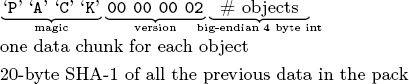
15:07.1 The Git Bundle File Format
The file format for Git bundles doesn’t appear to be formally specified anywhere, however, inspecting bundle.c reveals that it’s relatively straightforward:

Git has another custom format called a Packfile that it uses to compress the objects in its database, as well as to reduce network bandwidth when pushing and pulling. The packfile is therefore an obvious choice for storing objects inside bundles. This of course raises the question: What is the format for a Git Packfile?
Git does have some internal documentation,0 however, it is rather sparse, and does not provide enough detail to fully parse the format. The documentation also has some “observations” that suggest it wasn’t even written by the file format’s creator and instead was written by a developer who was later trying to make sense of the code.
Luckily, Aditya Mukerjee already had to reverse engineer the file format for his GitGo clean-room implementation of Git, and he wrote an excellent blog entry about it.1
Although not entirely required to understand the polyglot, I think it is useful to describe the git packfile format here, since it is not well documented elsewhere. If that doesn’t interest you, it’s safe to skip to the next section. But if you do proceed, I hope you like Soviet holes, dear neighbor, because chasing this rabbit might remind you of ![]() .
.
Right, the next step is to figure out the “chunk” format. The chunk header is variable length, and can be as small as one byte. It encodes the object’s type and its uncompressed size. If the object is a delta (i.e., a diff, as opposed to a complete object), the header is followed by either the SHA-1 hash of the base object to which the delta should be applied, or a byte reference within the packfile for the start of the base object. The remainder of the chunk consists of the object data, zlib-compressed.
The format of the variable length chunk header is pictured in Figure 15.14. The second through fourth most significant bits of the first byte are used to store the object type. The remainder of the bytes in the header are of the same format as bytes two and three in this example. This example header represents an object of type 112, which happens to be a git blob, and an uncompressed length of (1002 << 14) + (10101102 << 7) + 10010012 = 76,617 bytes. Since this is not a delta object, it is immediately followed by the zlib-compressed object data. The header does not encode the compressed size of the object, since the DEFLATE encoding

can determine the end of the object as it is being decompressed.
At this point, if you found The Life and Opinions of Tristram Shandy to be boring or frustrating, then it’s probably best to skip to the next section, ’cause it’s turtles all the way down.
“To come at the exact weight of things in the scientific fteel-yard, the fulchrum, [Walter Shandy] would say, should be almoft invisible, to avoid all friction from popular tenets;—without this the minutiæ of philosophy, which should always turn the balance, will have no weight at all. Knowledge, like matter, he would affirm, was divisible in infinitum;—that the grains and scruples were as much a part of it, as the gravitation of the whole world.”
There are two types of delta objects: references (object type 7) and offsets (object type 6). Reference delta objects contain an additional twenty bytes at the end of the header before the zlib-compressed delta data. These twenty bytes contain the SHA-1 hash of the base object to which the delta should be applied. Offset delta objects are exactly the same, however, instead of referencing the base object by its SHA-1 hash, it is instead represented by a negative byte offset to the start of the object within the pack file. Since a negative byte offset can typically be encoded in two or three bytes, it’s significantly smaller than a 20-byte SHA-1 hash. One must understand how these offset delta objects are encoded if—say, for some strange, masochistic reason—one wanted to change the order of objects within a packfile, since doing so would break the negative offsets. (Foreshadowing!)
One would think that git would use the same multi-byte length encoding that they used for the uncompressed object length. But
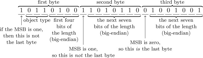
Figure 15.14: Format of the git packfile’s variable length chunk header.
no! This is what we have to go off of from the git documentation:
n bytes with MSB set in all but the last one.
The offset is then the number constructed by
concatenating the lower 7 bit of each byte, and
for n >= 2 adding 2^7 + 2^14 + ... + 2^(7*(n-1))
to the result.
Right. Some experimenting resulted in the following decoding logic that appears to work:
def decode_obj_ref(data):
bytes_read = 0
reference = 0
for c in map(ord, data):
bytes_read += 1
reference <<= 7
reference += c & 0b01111111
if not (c & 0b10000000):
break
if bytes_read >= 2:
reference += (1 << (7 * (bytes_read - 1)))
return reference, bytes_read
The rabbit hole is deeper still; we haven’t yet discovered the content of the compressed delta objects, let alone how they are applied to base objects. At this point, we have more than sufficient knowledge to proceed with the PoC, and my canary died ages ago. Aditya Mukerjee did a good job of explaining the process of applying deltas in his blog post, so I will stop here and proceed with the polyglot.
15:07.2 A Minimal Polyglot PoC
We now know that a git bundle is really just a git packfile with an additional header, and a git packfile stores individual objects using zlib, which uses the DEFLATE compression algorithm. DEFLATE supports zero compression, so if we can store the PDF in a single object (as opposed to it being split into deltas), then we could theoretically coerce it to be intact within a valid git bundle.
Forcing the PDF into a single object is easy: We just need to add it to the repo last, immediately before generating the bundle.
Getting the object to be compressed with zero compression is also relatively easy. That’s because git was built in almost religious adherence to The UNIX Philosophy: It is architected with hundreds of sub commands it calls “plumbing,” of which the vast majority you will likely have never heard. For example, you might be aware that git pull is equivalent to a git fetch followed by a git merge. In fact, the pull code actually spawns a new git child process to execute each of those subcommands. Likewise, the git bundle command spawns a git pack-objects child process to generate the packfile portion of the bundle. All we need to do is inject the --compression=0 argument into the list of command line arguments passed to pack-objects. This is a one-line addition to bundle.c:
argv_array_pushl(
&pack_objects.args,
"pack-objects", "--all-progress-implied",
"--compression=0",
"--stdout", "--thin", "--delta-base-offset",
NULL);
Using our patched version of git, every object stored in the bundle will be uncompressed!
$ export PATH=/path/to/patched/git:$PATH
$ git init
$ git add article.pdf
$ git commit article.pdf -m "added"
$ git bundle create PDFGitPolyglot.pdf --all
Any vanilla, un-patched version of git will be able to clone a repo from the bundle. It will also be a valid PDF, since virtually all PDF readers ignore garbage bytes before and after the PDF.
15:07.3 Generalizing the PoC
There are, of course, several limitations to the minimal PoC given in the previous section:
- Adobe, being Adobe, will refuse to open the polyglot unless the PDF is version 1.4 or earlier. I guess it doesn’t like some element of the git bundle signature or digest if it’s PDF 1.5. Why? Because Adobe, that’s why.
- Leaving the entire Git bundle uncompressed is wasteful if the repo contains other files; really, we only need the PDF to be uncompressed.
- If the PDF is larger than 65,535 bytes—the maximum size of an uncompressed DEFLATE block—then git will inject 5-byte deflate block headers inside the PDF, likely corrupting it.
- Adobe will also refuse to open the polyglot unless the PDF is near the beginning of the packfile.2
The first limitation is easy to fix by instructing LATEX to produce a version 1.4 PDF by adding pdfminorversion=4 to the document.
The second limitation is a simple matter of software engineering, adding a command line argument to the git bundle command that accepts the hash of the single file to leave uncompressed, and passing that hash to git pack-objects. I have created a fork of git with this feature.3
As an aside, while fixing the second limitation I discovered that if a file has multiple PDFs concatenated after one another (i.e., a git bundle polyglot with multiple uncompressed PDFs in the repo), then the behavior is viewer-dependent: Some viewers will render the first PDF, while others will render the last. That’s a fun way to generate a PDF that displays completely different content in, say, macOS Preview versus Adobe.
The third limitation is very tricky, and ultimately why this polyglot was not used for the PDF of this issue of PoC∥GTFO. I’ve a solution, but it will not work if the PDF contains any objects (e.g., images) that are larger than 65,535 bytes. A universal solution would be to break up the image into smaller ones and tile it back together, but that is not feasible for a document the size of a PoC∥GTFO issue.
DEFLATE headers for uncompressed blocks are very simple: The first byte encodes whether the following block is the last in the file, the next two bytes encode the block length, and the last two bytes are the ones’ complement of the length. Therefore, to resolve this issue, all we need to do is move all of the DEFLATE headers that zlib created to different positions that won’t corrupt the PDF, and update their lengths accordingly.
Where can we put a 5-byte DEFLATE header such that it won’t corrupt the PDF? We could use our standard trick of putting it in a PDF object stream that we’ve exploited countless times before to enable PoC∥GTFO polyglots. The trouble with that is: Object streams are fixed-length, so once the PDF is decompressed (i.e., when a repo is cloned from the git bundle), then all of the 5-byte DEFLATE headers will disappear and the object stream lengths would all be incorrect. Instead, I chose to use PDF comments, which start at any occurrence of the percent sign character (%) outside a string or stream and continue until the first occurrence of a newline. All of the PDF viewers I tested don’t seem to care if comments include non-ASCII characters; they seem to simply scan for a newline. Therefore, we can inject “% ” between PDF objects and move the DEFLATE headers there. The only caveat is that the DEFLATE header itself can’t contain a newline byte (0x0A), otherwise the comment would be ended prematurely. We can resolve that, if needed, by adding extra spaces to the end of the comment, increasing the length of the following DEFLATE block and thus increasing the length bytes in the DEFLATE header and avoiding the 0x0A. The only concession made with this approach is that PDF Xref offsets in the deflated version of the PDF will be off by a multiple of 5, due to the removed DEFLATE headers. Fortunately, most PDF readers can gracefully handle incorrect Xref offsets (at the expense of a slower loading time), and this will only affect the PDF contained in the repository, not the PDF polyglot.
As a final step, we need to update the SHA-1 sum at the end of the packfile (q.v. Section 15:07.1), since we moved the locations of the DEFLATE headers, thus affecting the hash.
At this point, we have all the tools necessary to create a generalized PDF/Git Bundle polyglot for almost any PDF and git repository. The only remaining hurdle is that some viewers require that the PDF occur as early in the packfile as possible. At first, I considered applying another patch directly to the git source code to make the uncompressed object first in the packfile. This approach proved to be very involved, in part due to git’s UNIX design philosophy and architecture of generic code reuse. We’re already updating the packfile’s SHA-1 hash due to changing the DEFLATE headers, so instead I decided to simply reorder the objects after-the-fact, subsequent to the DEFLATE header fix but before we update the hash. The only challenge is that moving objects in the packfile has the potential to break offset delta objects, since they refer to their base objects via a byte offset within the packfile. Moving the PDF to the beginning will break any offset delta objects that occur after the original position of the PDF that refer to base objects that occur before the original position of the PDF. I originally attempted to rewrite the broken offset delta objects, which is why I had to dive deeper into the rabbit hole of the packfile format to understand the delta object headers. (You saw this at the end of Section 15:07.1, if you were brave enough to finish it.) Rewriting the broken offset delta objects is the correct solution, but, in the end, I discovered a much simpler way.
“As a matter of fact, G-d just questioned my judgment. He said, Terry, are you worthy to be the man who makes The Temple? If you are, you must answer: Is this [dastardly], or is this divine intellect?”
—Terry A. Davis, creator of TempleOS and self-proclaimed “smartest programmer that’s ever lived”
Terry’s not the only one who’s written a compiler!
In the previous section, recall that we created the minimal PoC by patching the command line arguments to pack-objects. One of the command line arguments that is already passed by default is --delta-base-offset. Running git help pack-objects reveals the following:
A packed archive can express the base object
of a delta as either a 20-byte object name
or as an offset in the stream, but ancient
versions of Git don’t understand the latter.
By default, git pack-objects only uses the
former format for better compatibility. This
option allows the command to use the latter
format for compactness. Depending on the
average delta chain length, this option
typically shrinks the resulting packfile by
3-5 per-cent.
So all we need to do is remove the --delta-base-offset argument and git will not include any offset delta objects in the pack!
__________________________
Okay, I have to admit something: There is one more challenge. You see, the PDF standard (ISO 32000-1) says
“The trailer of a PDF file enables a conforming reader to quickly find the cross-reference table and certain special objects. Conforming readers should read a PDF file from its end. The last line of the file shall contain only the end-of-file marker, %%EOF.”
Granted, we are producing a PDF that conforms to version 1.4 of the specification, which doesn’t appear to have that requirement. However, at least as early as version 1.3, the specification did have an implementation note that Acrobat requires the %%EOF to be within the last 1024 bytes of the file. Either way, that’s not guaranteed to be the case for us, especially since we are moving the PDF to be at the beginning of the packfile. There are always going to be at least twenty trailing bytes after the PDF’s %%EOF (namely the packfile’s final SHA-1 checksum), and if the git repository is large, there are likely to be more than 1024 bytes.
Fortunately, most common PDF readers don’t seem to care how many trailing bytes there are, at least when the PDF is version 1.4. Unfortunately, some readers such as Adobe’s try to be “helpful,” silently “fixing” the problem and offering to save the fixed version upon exit. We can at least partially fix the PDF, ensuring that the %%EOF is exactly twenty bytes from the end of the file, by creating a second uncompressed git object as the very end of the packfile (right before the final twenty byte SHA-1 checksum). We could then move the trailer from the end of the original PDF at the start of the pack to the new git object at the end of the pack. Finally, we could encapsulate the “middle” objects of the packfile inside a PDF stream object, such that they are ignored by the PDF. The tricky part is that we would have to know how many bytes will be in that stream before we add the PDF to the git database. That’s theoretically possible to do a priori, but it’d be very labor intensive to pull off. Furthermore, using this approach will completely break the inner PDF that is produced by cloning the repository, since its trailer will then be in a separate file. Therefore, I chose to live with Adobe’s helpfulness and not pursue this fix for the PoC.
The feelies contain a standalone PDF of this article that is also a git bundle containing its LATEX source, as well as all of the code necessary to regenerate the polyglot.4 Clone it to take a look at the history of this article and its associated code! The code is also hosted on GitHub.5
Thus—thus, my fellow-neighbours and affociates in this great harveft of our learning, now ripening before our eyes; thus it is, by flow fteps of cafual increafe, that our knowledge phyfical, metaphyfical, phyfiological, polemical, nautical, mathematical, ænigmatical, technical, biographical, romantical, chemical, obftetrical, and polyglottical, with fifty other branches of it, (moft of ’em ending as thefe do, in ical) have for thefe four laft centuries and more, gradually been creeping upwards towards that Akme of their perfections, from which, if we may form a conjecture from the advances of thefe laft 15 pages, we cannot poffibly be far off.
POC-1337 Page 307 |
INSTRUMENTS |
|
Cyberencabulator |
||
Jan. 1, 1970 |
||
FUNCTION To measure inverse reactive current in universal phase detractors with display of percent realization. OPERATION Based on the principle of power generation by the modial interaction of magnetoreluctance and capacitative diractance, the Cyberencabulator negates the relative motion of conventional conductors and fluxes. It consists of a baseplate of prefabulated Amulite, surmounted by a malleable logarithmic casing in such a way that the two main spurving bearings are aligned with the parametric fan. Six gyro-controlled antigravic marzelvanes are attached to the ambifacent wane shafts to prevent internal precession. Along the top, adjacent to the panandermic semi-boloid stator slots, are forty-seven manestically spaced grouting brushes, insulated with Glyptalimpregnated, cyanoethylated kraft paper bushings. Each one of these feeds into the rotor slip-stream, via the non-reversible differential tremie pipes, a 5 per cent solution of reminative Tetraethyliodohexamine, the specific pericosity of which is given by The two panel meters display inrush current and percent realization. In addition, whenever a barescent skor motion is required, it may be employed with a reciprocating dingle arm to reduce the sinusoidal depleneration in nofer trunions. Solutions are checked via Zahn Viscosimetry techniques. Exhaust orifices receive standard Blevinometric tests. There is no known Orth Effect. TECHNICAL FEATURES
STANDARD RATINGS  * Included Qty. 6 NO-BLO‡ fuses. † Includes Magnaglas circuit breaker with polykrapolene-coated contacts rated 75A Wolfram. ‡ Reg. T.M. Shenzhen Xiao Baoshi Electronics Co., Ltd. ACCESSORIES
APPLICATION Measuring Inverse Reactive Current—CAUTION: Because of the replenerative flow characteristics of positive ions in unilateral phase detractors, the use of the quasistatic regeneration oscillator is recommended if Cyberencabulator is used outside of an air conditioned server room. Reduction of Sinusoidal Depleneration —Before use, the system should be calibrated with a gyro-controlled Sine-Wave Director, the output of which should be of the cathode follower type. Note: If only Cosine-Wave Directors are available, their output must be first fed into a Phase Inverter with parametric negative-time compensators. Caution: Only Phase Inverters with an output conductance of 17.8 ± 1 millimhos should be employed so as to match the characteristics of the quasistatic regeneration oscillator. Voltage Levels—Above 750V Do Not Use Caged Resistors to get within self-contained rating of Cyberencabulator. Do Use Sequential Transformers. See POC-9001. Multiple Ratings—Optionally available in multiples of π (22/7) and e (19/7). If binary or other number-base systems ratios are required, refer to the fuctoría for availability and pricing. Goniometric Data—Upon request, curves are supplied, at additional charge, for regions wherein the molecular MFP (Mean Free Path) is between 1.6 and 19.62 Angstrom units. Curves, relevant to regions outside the abovelisted range, may be obtained from: Tract Association of PoC∥GTFO and Friends, GmbH Cloud Computing Cyberencabulator Dept. (C3D) Tennessee, ‘Murrica In Canada address request to: Cyberencabulateurs Canaderpien-Français Ltée. 468 Jean de Quen, Quebec 10, P.Q. Reference Texts
SPECIFICATIONS Accuracy: ±1 per cent of point Repeatability: ±¼ per cent Maintenance Required: Bimonthly treatment of Meter covers with Shure Stat. Ratings: None (Standard); All (Optional) Fuel Efficiency: 1.337 Light-Years per Sydharb Input Power: Volts—120/240/480/550 AC Amps—10/5/2.5/2.2 A Watts—1200 W Wave Shape—Sinusoidal, Cosinusoidal, Tangential, or Pipusoidal. Operating Environment: Temperature 32F to 150F (0C to 66C) Max Magnetic Field: 15 Mendelsohns (1 Mendelsohn = 32.6 Statoersteds) Case: Material: Amulite; Tremie-pipes are of Chinesium—(Tungsten Cowhide) Weight: Net 134 lbs.; Ship 213 lbs. DIMENSION DRAWINGS On delivery. EXTERNAL WIRING On delivery. Data subject to change without notice |
||
15:08 Zero Overhead Networking
by Robert Graham
The kernel is a religion. We programmers are taught to let the kernel do the heavy lifting for us. We the laity are taught how to propitiate the kernel spirits in order to make our code go faster. The priesthood is taught to move their code into the kernel, as that is where speed happens.
This is all a lie. The true path to writing high-speed network applications, like firewalls, intrusion detection, and port scanners, is to completely bypass the kernel. Disconnect the network card from the kernel, memory map the I/O registers into user space, and DMA packets directly to and from user-mode memory. At this point, the overhead drops to near zero, and the only thing that affects your speed is you.
Masscan
Masscan is an Internet-scale port scanner, meaning that it can scan the range /0. By default, with no special options, it uses the standard API for raw network access known as libpcap. Libpcap itself is just a thin API on top of whatever underlying API is needed to get raw packets from Linux, macOS, BSD, Windows, or a wide range of other platforms.
But Masscan also supports another way of getting raw packets known as PF_RING. This runs the driver code in user-mode. This allows Masscan to transmit packets by sending them directly to the network hardware, bypassing the kernel completely. No memory copies, no kernel calls. Just put “zc:” (meaning PF_RING ZeroCopy) in front of an adapter name, and Masscan will load PF_RING if it exists and use that instead of libpcap.
In the following section, we are going to analyze the difference in performance between these two methods. On the test platform, Masscan transmits at 1.5 million packets-per-second going through the kernel, and transmits at 8 million packets-per-second when going though PF_RING.
We are going to run the Linux profiling tool called perf to find out where the CPU is spending all its time in both scenarios.
Raw output from perf is difficult to read, so the results have been processed through Brendan Gregg’s FlameGraph tool. This shows the call stack of every sample it takes, showing the total time in the caller as well as the smaller times in each function called, in the next layer. This produces SVG files, which allow you to drill down to see the full function names, which get clipped in the images.
I first run Masscan using the standard libpcap API, which sends packets via the kernel, the normal way. Doing it this way gets a packet rate of about 1.5 million packets-per-second, as shown on page 310.
To the left, you can see how perf is confused by the call stack, with [unknown] functions. Analyzing this part of the data shows the same call stacks that appear in the central section. Therefore, assume all that time is simply added onto similar functions in that area, on top of __libc_send().
The large stack of functions to the right is perf profiling itself. In the section to the right where Masscan is running, you’ll notice little towers on top of each function call. Those are the interrupt handlers in the kernel. They technically aren’t part of Masscan, but whenever an interrupt happens, registers are pushed onto the stack of whichever thread is currently running. Thus, with high enough resolution (faster samples, longer profile duration), perf will count every function as having spent time in an interrupt handler.

1 marks the start of entry_SYSCALL_64_fastpath(), where the machine transitions from user to kernel mode. Everything above this is kernel space. That’s why we use perf rather than user-mode profilers like gprof, so that we can see the time taken in the kernel.
2 marks the function packet_sendmsg(), which does all the work of sending the packet.
3 marks sock_alloc_send_pskb(), which allocates a buffer for holding the packet that’s being sent. (skb refers to sk_buff, the socket buffer that Linux uses everywhere in the network stack.)
4 marks the matching function consume_skb(), which releases and frees the sk_-buff. I point this out to show how much of the time spent transmitting packets is actually spent just allocating and freeing buffers. This will be important later on.
Performance profile of Masscan with libpcap.
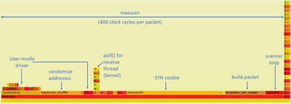
Figure 15.15: Performance profile of Masscan with PF_RING.
The next run of Masscan bypasses the kernel completely, replacing the kernel’s Ethernet driver with the user-mode driver PF_RING. It uses the same options, but adds “zc:” in front of the adapter name. It transmits at 8 million packets-per-second, using an Ivy Bridge processor running at 3.2 GHz (turboed up from 2.5 GHz). Shown in Figure 15.15, this results in just 400 cycles per packet!
The first thing to notice here is that 3.2 GHz divided by 8 mpps equals 400 clock cycles per packet. If we looked at the raw data, we could tell how many clock cycles each function is taking.
Masscan sits in a tight scanner loop called transmit_thread(). This should really be below all the rest of the functions in this flame graph, but apparently perf has trouble seeing the full call stack.
The scanner loop does the following calculations:
- It randomizes the address in blackrock_shuffle()
- It calculates a SYN cookie using the siphash24() hashing function
- It builds the packet, filling in the destination IP/port, and calculating the checksum
- It then transmits it via the PF_RING user-mode driver
At the same time, the receive_thread() is receiving packets. While the transmit thread doesn’t enter the kernel, the receive thread will, spending most of its time waiting for incoming packets via the poll() system call. Masscan transmits at high rates, but receives responses at fairly low rates.
To the left, in two separate chunks, we see the time spent in the PF_RING user-mode driver. Here perf is confused: about a third of this time is spent in the receive thread, and the other two thirds are spent in the transmit thread.
About ten to fifteen percent of the time is taken up inside PF_RING user-mode driver or an overhead 40 clock cycles per packet.
Nearly half of the time is taken up by siphash24(), for calculating the SYN cookie. Masscan doesn’t remember which packets it has sent, but instead uses the SYN cookie technique to verify whether a response is valid. This is done by setting the Initial Sequence Number of the SYN packet to a hash of the IP addresses, port numbers, and a secret. By using a cryptographically strong hash, like siphash, it assures that somebody receiving packets cannot figure out that secret and spoof responses back to Mass-can. Siphash is normally considered a fast hash, and the fact that it’s taking so much time demonstrates how little the rest of the code is doing.
Building the packet takes ten percent of the time. Most of the this is spent needlessly calculating the checksum. This can be offloaded onto the hardware, saving a bit of time.
The most important point here is that the transmit thread doesn’t hit the kernel. The receive thread does, because it needs to stop and wait, but the transmit thread doesn’t. PF_RING’s custom user-mode driver simply reads and writes directly into the network hardware registers, and manages the transmit and receive ring buffers, all memory-mapped from kernel into user mode.
The benefits of this approach are that there is no system call overhead, and there is no needless copying of packets. But the biggest performance gain comes from not allocating and then freeing packets. As we see from the previous profile, that’s where the kernel spends much of its time.
The reason for this is that the network card is normally a shared resource. While Masscan is transmitting, the system may also be running a webserver on that card, and supporting SSH login sessions. Sharing these resources ultimately means allocating and freeing sk_buffs whenever packets are sent or received.
PF_RING, however, wrests control of the network card away from the kernel, and gives it wholly to Masscan. No other application can use the network card while Masscan is running. If you want to SSH into the box in order to run ![]() , you’ll need a second network card.
, you’ll need a second network card.
If Masscan takes 400 clock cycles per packet, how many CPU instructions is that? Perf can answer that question, with a call like perf -a sleep 100. It gives us an IPC (instructions per clock cycle) ratio of 2.43, which means around 1000 instructions per packet for Masscan.
To reiterate, the point of all this profiling is this: when running with libpcap, most of the time is spent in the kernel. With PF_RING, we can see from the profile graphs that the kernel is completely bypassed on the transmit thread. The overhead goes from most of the CPU to very little of the CPU. Any performance issues are in the Masscan, such as choosing a slow cryptographic hash algorithm instead of a faster, non-cryptographic algorithm, rather than in the kernel!
How to Replicate This Profiling
Here is brief guide to reproducing this article’s profile flamegraphs. This would be useful to compare against other network projects, other drivers, or for playing with Masscan to tune its speed. You may skip to page 317 on a first reading, but if, like me, you never trusted a graph you could not reproduce yourself, read on!
Get two computers. You want one to transmit, and another to receive. Almost any Intel desktop will do.
Buy two Intel 10gig Ethernet adapters: one to transmit, and the other to receive and verify the packets have been received. The adapters cost $200 to $300 each. They have to be the Intel chipset; other chipsets won’t work.
Install Ubuntu 16.04, as it’s the easiest system to get perf running on. I had trouble with other systems.
The perf program gets confused by idle threads. Therefore, for profiling, I rebooted the Linux computer with maxcpus=1 on the boot command line. I did this by editing /etc/default/grub, adding maxcpus=1 to the line GRUB_CMDLINE_LINUX_DEFAULT, then running update-grub to save the configuration.
To install perf, Masscan, and FlameGraph:

The pf_ring.ko module should load automatically on reboot, but you’ll need to rerun load_drivers.sh every time. If I ran this in production, rather than just for testing, I’d probably figure out the best way to auto-load it.
You can set all the parameters for Masscan on the command line, but it’s easier to create a default configuration file in /etc/-masscan/masscan.conf:
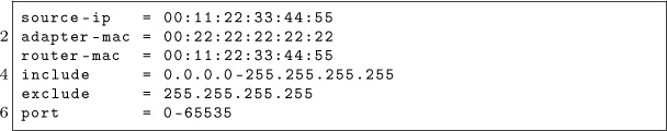
Since there is no network stack attached to the network adapter, we have to fake one of our own. Therefore, we have to configure that source IP and MAC address, as well as the destination router MAC address. It’s really important that you have a fake router MAC address, in case you accidentally cross-connect your 10gig hub with your home network and end up blasting your Internet connection. (This has happened to me, and it’s no fun!)
Now we run Masscan. For the first run, we’ll do the normal adapter without PF_RING. Pick the correct network adapter for your machine. On my machine, it’s enp2s03.
masscan -e enp2s0f1 - rate 100000000
In another window, run the following. This will grab 99 samples per second for 60 seconds while Masscan is running. A minute later, you will have an SVG of the flamegraphs.
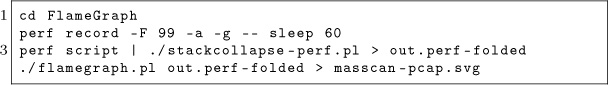
Now, repeat the process to produce masscan-pfring.svg with the following command. It’s the same as the original Mass-can run, except that we’ve prefixed the adapter name with zc:. This disconnects any kernel network stack you might have on the adapter and instead uses the user-mode driver in the libpfring.so library that Masscan will load:
masscan -e zc : enp2s0f1 - rate 100000000
At this point, you should have two FlameGraphs. Load these in any web browser, and you can drill down into the specific functions.
Playing with perf options, or using something else like dtrace, might produce better results. The results I get match my expectations, so I haven’t played with them enough to test their accuracy. I challenge you to do this, though—for reproducibility is the heart and soul of science. Trust no one; reproduce everything you can.
Now back to our regular programming.

How Ethernet Drivers Work
If you run lspci -v for the Ethernet cards, you’ll see something like the following.
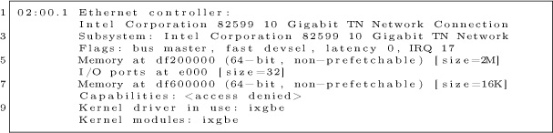
There are five parts to notice.
- There is a small 16k memory region. This is where the driver controls the card, using memory-mapped I/O, by reading and writing these memory addresses. There’s no actual memory here—these are registers on the card. Writes to these registers cause the card to do something, reads from this memory check status information.
- There is a small amount of I/O ports address space reserved. It points to the same registers mapped in memory. Only Intel x86 processors support a second I/O space along with memory space, using the inb/outb instructions to read and write in this space. Other CPUs (like ARM) don’t, so most devices also support memory-mapped I/O to these same registers. For user-mode drivers, we use memory-mapped I/O instead of x86’s “native” inb/outb I/O instructions.
- There is a large 2MB memory region. This memory is used to store descriptors (pointers) to packet buffers in main memory. The driver allocates memory, then writes (via memory-mapped I/O) the descriptors to this region.
- The network chip uses Bus Master DMA. When packets arrive, the network chip chooses the next free descriptor and DMAs the packet across the PCIe bus into that memory, then marks the status of the descriptor as used.
- The network chip can (optionally) use interrupts (IRQs) to inform the driver that packets have arrived, or that transmits are complete. Interrupt handlers must be in kernel space, but the Linux user-mode I/O (UIO) framework allows you to connect interrupts to file handles, so that the user-mode code can call the normal poll() or select() to wait on them. In Masscan, the receive thread uses this, but the interrupts aren’t used on the transmit thread.
There is also some confusion about IOMMU. It doesn’t control the memory mapped I/O; that goes through the normal MMU, because it’s still the CPU that’s reading and writing memory. Instead, the IOMMU controls the DMA transfers, when a PCIe device is reading or writing memory.
Packet buffers/descriptors are arranged in a ring buffer. When a packet arrives, the hardware picks the next free descriptor at the head of the ring, then moves the head forward. If the head goes past the end of the array of descriptors, it wraps around at the beginning. The software processes packets at the tail of the ring, likewise moving the tail forward for each packet it frees. If the head catches up with the tail, and there are no free descriptors left, then the network card must drop the packet. If the tail catches up with the head, then the software is done processing all the packets, and must either wait for the next interrupt, or if interrupts are disabled, must keep polling to see if any new packets have arrived.
Transmits work the same way. The software writes descriptors at the head, pointing to packets it wants to send, moving the head forward. The hardware grabs the packets at the tail, transmits them, then moves the tail forward. It then generates an interrupt to notify the software that it can free the packet, or, if interrupts are disabled, the software will have to poll for this information.
In Linux, when a packet arrives, it’s removed from the ring buffer. Some drivers allocate an sk_buff, then copy the packet from the ring buffer into the sk_buff. Other drivers allocate an sk_buff, and swap it with the previous sk_buff that holds the packet.
Either way, the sk_buff holding the packet is now forwarded up through the network stack, until the user-mode app does a recv()/read() of the data from the socket. At this point, the sk_buff is freed.
A user-mode driver, however, just leaves the packet in place, and handles it right there. An IDS, for example, will run all of its deep-packet-inspection right on the packet in the ring buffer.
Logically, a user-mode driver consists of two steps. The first is to grab the pointer to the next available packet in the ring buffer. Then it processes the packet, in place. The next step is to release the packet. (Memory-mapped I/O to the network card to move the tail pointer forward.)
In practice, when you look at APIs like PF_RING, it’s done in a single step. The code grabs a pointer to the next available packet while simultaneously releasing the previous packet. Thus, the code sits in a tight loop calling pfring_recv() without worrying about the details. The pfring_recv() function returns the pointer to the packet in the ring buffer, the length, and the timestamp.
In theory, there’s not a lot of instructions involved in pfring_-recv(). Ring buffers are very efficient, not even requiring locks, which would be expensive across the PCIe bus. However, I/O has weak memory consistency. This means that although the code writes first A then B, sometimes the CPU may reorder the writes across the PCI bus to write first B then A. This can confuse the network hardware, which expects first A then B. To fix this, the driver needs memory fences to enforce the order. Such a fence can cost 30 clock cycles.
Let’s talk sk_buffs for the moment. Historically, as a packet passed from layer to layer through the TCP/IP stack, a copy would be made of the packet. The newer designs have focused on “zero-copy,” where instead a pointer to the sk_buff is forwarded to each layer. For drivers that allocate an sk_buff to begin with, the kernel will never make a copy of the packet. It’ll allocate a new sk_buff and swap pointers, rewriting the descriptor to point to the newly allocated buffer. It’ll then pass the received packet’s sk_buff pointer up through the network stack. As we saw in the FlameGraphs, allocating sk_buffs is expensive!
Allocating sk_buffs (or copying packets) is necessary in the Linux stack because the network card is a shared resource. If you left the packets in the ring buffer, then one slow app that leaves the packet there would eventually cause the ring buffer to fill up and halt, affecting all the other applications on the system. Thus, when the network card is shared, packets need to be removed from the ring. When the network card is a dedicated resource, packets can just stay in the ring buffer, and be processed in place.
Let’s talk zero-copy for a moment. The Linux kernel went through a period where it obsessively removed all copying of packets, but there’s still one copy left: the point where the user-mode application calls recv() or read() to read the packet’s contents. At that point, a copy is made from kernel-mode memory into user-mode memory. So the term zero-copy is, in fact, a lie whenever the kernel is involved!
With user-mode drivers, however, zero-copy is the truth. The code processes the packet right in the ring buffer. In an application like a firewall, the adapter would DMA the packet in on receive, then out on transmit. The CPU would read from memory the packet headers to analyze them, but never read the payload. The payload will pass through the system completely untouched by the CPU.
Let’s talk about interrupts for a moment. Back in the day, an interrupt was generated per packet. Indeed, at one time, two interrupts could be generated, one after the TCP/IP headers were received, so processing could start immediately, and another after the rest of the packet had been received.
The value of interrupts is that they provide low latency, important for devices that forward packets (firewalls, IPS, routers), or for fast responses to packets. The cost of interrupts, though, is that they cause large CPU overhead. When an interrupts happens, it forces execution of an interrupt handler. Even medium rates of packets can overwhelm the system with interrupts, so that as soon as the system leaves an interrupt handler, it immediately enters another one. In such cases, the system has essentially locked up. The mouse won’t even move on the screen until the packet rate decreases, after which point the system will behave normally.0
The obvious solution to this is to turn off interrupts from the network card. Instead, the software can sit in a tight loop and poll() to see if new packets arrive. Another strategy is to program the timer chip for frequent interrupts. The card can bounce back and forth among these strategies, depending on the current network speed. Polling consumes a lot of CPU time. Using delayed timer interrupts increases latency.
Those writing custom drivers have used these strategies since the 1980s. Around 2006, Linux drivers started doing the same, using the NAPI API to enable polling when packets arrived at high speed. Around that time, network hardware also improved, adding support for coalescing interrupts, so that it generated fewer at high speed, generating only one interrupt after many packets have arrived.
In the graphs, you saw that the libpcap had some small overhead with interrupts, but it’s not overwhelming, because NAPI interrupt moderation kicks in. Using pfring gets rid of this overhead.
Let’s talk system call overhead. A recent paper by Livio Soares and Michael Stumm does a good job measuring it.1 The basic cost of entering or leaving kernel space is around 150 clock cycles. This alone takes more time than all the user-mode driver processing done by PF_RING, according to our measurements.
There are further expenses to the system call. It has to walk through a bunch of kernel data structures. This then pollutes the caches on the chip. According to the Soares paper, it evicts about half the data in the L1 cache. This will cause data access to go from 4 clock cycles (often masked by the out-of-order processing of the CPU) to 12 clocks in L2 cache, or 30 clocks in L3 cache. The effective cost can thus equal hundreds of extra clock cycles.
On the other hand, the cost can easily be amortized by doing multiple packet reads or writes per system call. Linux has a recvmsg() system call that does this, to good effect.
Combining all this together, we see why a user-mode driver has such big gains (or conversely, why the kernel has such big losses): (a) it avoids the allocation/deallocation of memory; (b) it avoids any memory copies; (c) it avoids system call overhead, and (d) it avoids interrupts.
Some History of Ethernet Drivers
Since the dawn of networking there have been people dissatisfied with the standard Ethernet drivers who have written their own.
An example were packet sniffers, like the Network General “Sniffer” product. Back in the day, they wrote custom drivers so they could capture at “wire speed” on an 80286 microprocessor. The major feature was simply disabling interrupts. Portable MS-DOS computers were used as packet sniffers because “real” computers like SPARCstations running Solaris couldn’t handle high traffic rates.
Early drivers were hard, because hardware sucked. There was no bus master DMA in the early ISA bus days, so for DMA, you had to use the motherboard’s DMA controller. Only, it wasn’t really that fast. So instead, drivers used the Programmed I/O (PIO) mode to read packets from the adapter.
There was also the problem of bus bandwidth. Early PCI supported 1 Gbps in theory (32 bits times 33 MHz), but various overheads made that impractical. It wasn’t until wider PCI (64-bit) or/and faster PCI (66 MHz) that true wirespeed gigabit Ethernet was possible.
Also, with PCI, all the slots were shared on the same bus, so other devices impacted yours. This was especially difficult when building firewalls, routers, or IPS applications that needed to both transmit and receive. Luckily, motherboards started supporting multiple independent PCI buses. Still, PCI was still single-plexed, meaning it couldn’t transfer in both directions at the same time.
Virtually all these concerns have gone away now. Even a single lane of PCIe 1.0 is 2 Gbps, bidirectional, with more than enough bandwidth to handle sending and receiving at full 1 Gbps.
The early Intel 1 Gbps card had only 256 descriptors. Timing was tight enough that at full bandwidth; there wasn’t enough time to process packets before the ring buffer would fill up. With BlackICE, we solved this by allocating an effective ring buffer of several thousand descriptors. Then, when packets arrived, we replaced the existing descriptors with new descriptors from the preallocated set. We used two CPUs, one dedicated to running the user-mode driver doing this, and another reading and processing packets from the large virtual ring buffer. I mention this trick because, at the time, Intel engineers told us it wasn’t possible to capture packets at wirespeed, and we were able to prove them wrong.

Historically, and often today, the reality is that few hardware vendors test their hardware at maximum speed. Since operating systems can’t handle it, they don’t test for it. That makes writing drivers for practical hardware much harder than it would seem in theory, as driver writers have to overcome bugs in the hardware.
Today, custom drivers are common. Back in the day, they were black magic.

Core Concept
In 1998, I created BlackICE, an IDS/IPS using a custom driver. A frequent question at the time was why we didn’t write it on Linux, or even BSD, which everyone knew was faster. In particular, some papers at the time “proved” that the BSD networking was the fastest.
This bothered me because I was unable to explain the core concept. If we are completely bypassing the operating system, then the operating system doesn’t matter. As the graphs show, Masscan spends no time in the operating system. Given the same version of GCC, and the same hardware, it’ll run at nearly identical speed, regardless of whether the operating system is Windows, Linux, or BSD. It’s like any other CPU-bound (rather than OS-bound) task.
Yet, people couldn’t appreciate this. They knew in their hearts that some operating system was better, and couldn’t see the concept of bypassing it.
BlackICE used poll mode, instead of interrupts, so it didn’t lock up under high packet rates. Now, with NAPI, and poll-mode drivers like PF_RING, it’s something everyone can play with and understand. Back then, it was some weird black magic that people refused to believe actually worked. My 11-inch laptop computer happened to use 3Com’s 3c905 chip, the only 100 Mbps card we wrote a driver for. Even after demonstrating it handling the maximum rate of 148,800 packets-per-second, people refused to believe it worked.2 Nowadays, cheap notebooks easily handle max 1 Gbps speeds (1,488,000 packets-per-second) using things like PF_RING.
In 2003, Gartner came out with a report that software IDS was dead, because it couldn’t handle line-rate gigabit Ethernet, and that “hardware” was needed. That was based on experience with Snort, which had no custom drivers available at the time. Even when customers explained to Gartner they were successfully using our product at line rate, they refused to believe.
More interesting was the customers who tested our software product side-by-side with “hardware” competitors in the lab, and found our product faster. They still bought the competitors’, because of FUD. Nobody got fired for buying a hardware product that turned out to be slow.
Even today, discussions of these drivers still get questions like “What about Endace?” Endace builds custom cards with FPGAs to accelerate processing. This doesn’t apply. The overhead for Masscan using PF_RING is nearly zero, and would have the identical overhead working with an Endace card, also near zero. The FPGA doesn’t reach outside the card and somehow make Masscan’s code faster.
Yes, Endace does have some advantages. You can push filters to card, so that fewer packets arrive in a system. This is needed in some networks. However, most people use Endace for things that PF_RING would solve just fine, because they believe in the power of hardware.
Finally, the same sorts of prejudices exist with kernel code. Programmers are indoctrinated to believe code runs faster in the kernel, which is not true. The reason you push stuff into the kernel is to avoid the kernel/user transition. There’s otherwise no inherent advantage. Pushing things like the driver to user mode is just doing the same thing, avoiding the kernel/user transition. Indeed, that’s all micorokernels are, operating systems that aggressively push subsystems outside the kernel.
Several Drivers to Choose From
Masscan uses PF_RING because of compile dependencies; there is no actual dependency. You compile Masscan without any dependency on PF_RING, yet that compiled code will go hunt for the pfring.so library and dynamically load it. Thus, in the replication instructions, I have you compile Masscan first, and PF_RING second. But there are two other options of note.
Intel has a system called DPDK, the Data-Plane Development Kit. It contains not only a user-mode driver similar to PF_RING, but a whole toolkit to solve other problems, like multi-CPU synchronization and multi-socket NUMA memory handling. It’s a real awesome toolkit. However, it’s also an enormous dependency for code. That’s why Masscan uses PF_RING—it’s an optional feature that most users will never see. Had I used DPDK, I would’ve forced users into dependency hell trying to build a massive toolkit for my little application.
Another option is netmap. This is a kernel-mode driver that is otherwise identical to the user-mode stuff. It memory maps the packet buffers in user space, so it’s truly zero copy. It also disconnects the driver from the network stack, and gives exclusive access to the application, so there’s no allocation and freeing of sk_buffs. It batches multiple reads and writes with a single system call, amortizing the cost of system calls across many packets.
The great thing about netmap is that it’s built into the latest Linux kernels. Assuming you have Intel Ethernet, or even a Realtek Gigabit card, it should work immediately with no special software. I haven’t gotten around to adding this to Masscan, but the overhead should be comparable to PF_RING—despite being tainted with evil kernel-mode code.
Some notes on IDS design
One place to use these “user-mode no-interrupt zero-copy ringbuffer” drivers is with a network intrusion detection system, or even an inline version called and intrusion prevention system.
None of the existing open-source IDS projects (Snort, Bro, Suricata) are really designed for speed. They were written using libpcap where, at high speed, the kernel consumed most of the CPU power. As a consequence, there were only so much performance improvements that could be made before it wasn’t worth it. Optimizations that made the software infinitely fast would still not even double the practical performance of the IDS, because the kernel would be eating up all the time.
But, with near zero overhead in the drivers, some interesting optimizations become worthwhile.
One problem with the Snort IDS is how it does TCP reassembly. It must copy packets into the same buffer in order to perform regex searches. This adds two things which we know to be bad: memory allocations and memory copies. An alternative is to not do this, to neither do regex as the basis of signatures, nor do reassembly.
This approach is demonstrated in Masscan in several places. Masscan can establish a TCP connection and interact with the service. When it needs to search for patterns, instead of a regex it uses an Aho-Corasick (AC) pattern matcher. Whereas a normal regex needs to have a complete buffer, so that it can do back tracking, an AC pattern matcher does not. It accepts input a
sequence of fragments, saving the state of the search at the end of one fragment and continuing at the start of the next fragment.
This has the same practical ability to search a TCP stream, but without the need to “reassemble” fragments, allocate memory, or do memory copies.
In abstract computer science terms, this is the trade-off between NFAs (non-deterministic finite automata) which can consume a lot of CPU power, and DFAs (deterministic finite automata), which consume a fixed amount of CPU power, but at the expense of using a lot of memory for the tables it builds.
Another thing you’ll see in Masscan is protocol decoders based on state machines. Again, instead of reassembling packets, the protocol decoder saves state at the end of one fragment and continues with that state at the start of the next. An example of this is the X.509 parser, proto-x509.c. The unit test calls this two ways, one with an entire certificate to be parsed, and one where the bytes are processed one at a time, as if they had arrived in fragments over TCP.
Such state-machine parsers are really weird, but by avoiding memory allocations and copies, they become really fast at high network speeds. It’s a difficult optimization to make the code that would add little value when using kernel mode drivers, but becomes an important way of building an IDS if using these zero-overhead drivers.
The kernel is a lie.

15:09 Detecting MIPS16 Emulation
by Ryan Speers and Travis Goodspeed with the kindest of thanks to Thorsten Haas.
Howdy y’all,
Let’s begin with a joke that I once heard at a conference: David Patterson and John Hennessy walk into a bar. Everyone gathers to listen to the two heroes who built legendary machines. The entire bar spends the night multiplying fractions, and then everyone has that terrible hangover you get when you realize you had no fun and learned nothing new, even though your night started out so promising.
But let’s tell the joke differently: Patterson and Hennessy walk into a bar in another town, but this time, Greg Peterson is behind the bar. The two of them begin a long-winded story about weighted averages, lashing out at “RISC-deniers” who aren’t even in the room. Just as folks begin to get bored, and begin to sip their drinks too quickly out of nervousness, Peterson jumps in and saves the day. Because he knows that these fine folks built real machines that really shipped, he redirects the conversation to war stories and practical considerations.
Patterson tells how the two-stage pipeline in the RISC 1 chip was the first design with a branch delay slot, as there’s no point in throwing away the staged instruction that has already finished execution. Hennessy jumps in with a tale of dual instruction sets on MIPS, allowing denser code without abandoning the spirit of the RISC faith. Then Peterson, the bartender, serves up a number of Xilinx devkits to bar patrons, who begin collaborating on a five-stage pipeline design of their own, with advice on specific design choices from David and John. The next morning, they’ve built a working CPU and suffered no hangovers.
If your Computer Architecture class was more like the former than the latter, I hope that this brief article will show you some of the joy of this fine subject.
In PoC∥GTFO 6:6, Craig Heffner discussed a variety of methods for detecting Qemu emulation of MIPS hardware. We’ll be discussing one more way to detect emulation, but we’ll be using the MIPS16 instruction set and a clever trick of delay slots to detect the emulation.
We wanted to craft a capability that is (a) able to differentiate hardware from an emulation environment, and also (b) able to confuse static analysis. We used standard tools: Qemu as an emulation environment and IDA Pro as a disassembler.0
The first criterion leads us to want something that both (a) works in userland, and (b) is not trivial for an emulator developer to patch. Moving to userland meant that hardware registry inspection, as discussed in Section 6.1 of Heffner’s article, would not work. Similarly, the technique of reading cpuinfo in Section 6.2 would be easily patchable, as Craig noted. Here, we instead seek a capability more similar to Section 6.3, where cache incoherency is exploited to differentiate real hardware and Qemu.
MIPS16e
SSH’ing to a newly acquired MIPS box, we find the same nifty line of cpuinfo that struck our fancy in Craig’s article. MIPS16 is an extension to the classic MIPS instruction set that fills the same niche as Thumb2 does on ARM. The instructions word is 16 bits wide, a subset of the full register set is directly available, and a core tenet of RISC is violated: some instructions are more than one word long.
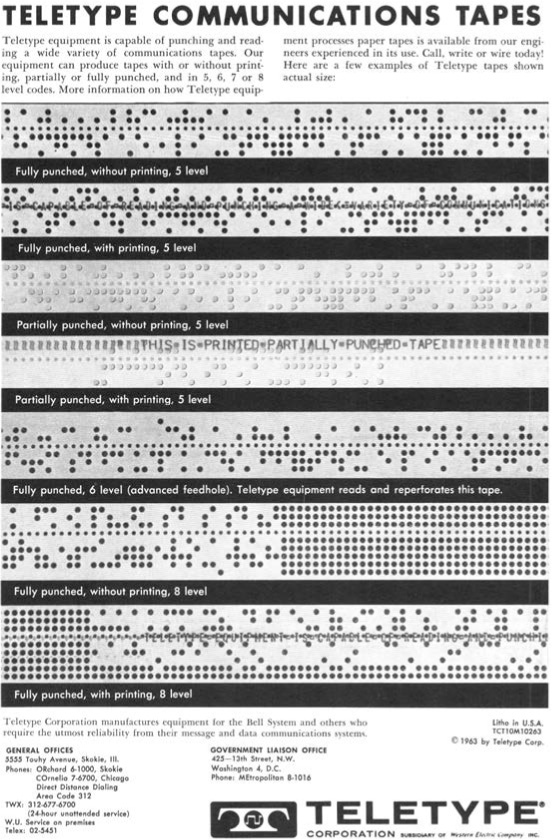
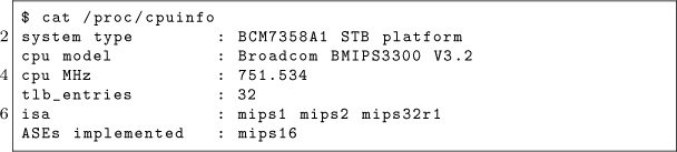
Just like ARM, this alternate instruction set is used whenever the least significant bit of the program counter is set. Function pointers work as expected between the two instruction sets, and the calling conventions are compatible.
Despite careful work to maintain compatibility between MIPS16 and MIPS32, there are inevitable differences. MIPS16 only has direct access to eight registers, rather than the 32 of its larger cousin.
CPU Pipelines
In Hennessy and Patterson’s books, a five-stage pipeline is described and hammered into the poor reader’s head. This classic RISC pipeline isn’t what you’ll find in modern chips, but it’s a lot easier to keep in mind while working on them. The stages in order are Instruction Fetch (IF), Instruction Decode (ID), Execute (EX), Memory Access (MEM), and Write Back (WB).
Each pipeline stage can only hold one instruction at a time, but by passing the instructions through as a queue, multiple instructions can exist in different stages at the same time. When a branch is mis-predicted, the pipeline will be “flushed,” which is to say that the partially-completed instructions from the incorrectly guessed branch are blown to the wind and replaced with harmless NOP instructions, which are sometimes called “bubbles.”
Bubbles are also one way to avoid “data hazards,” which are dependencies between instructions that run at the same time.
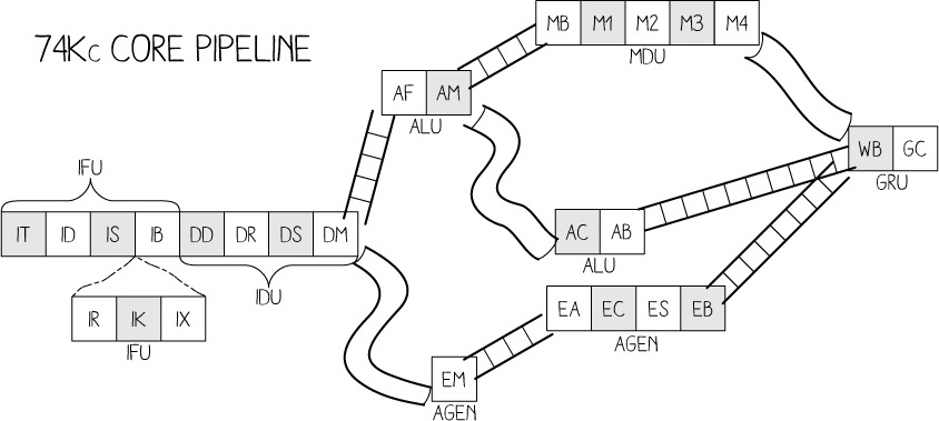
For example, if you were to use a value just after loading it, the CPU would have to either insert a bubble to delay the second instruction until the value is ready or it would “forward” the register result.1
The MIPS 74Kc on one of our target machines has 14 or 15 pipeline stages, depending upon how you count, plus three additional stages for MIPS16e instruction decoding.2 These stages are quite well documented, but to ease the explanation a bit, we won’t bore you with the details of exactly what happens where. The stages themselves are shown on page 336, helpfully illustrated by Ange Albertini.
Extended (Wide) Instructions
We mentioned earlier that MIPS16 instructions are usually just one instruction word, but that sometimes they are two. That’s a bit vague and hand-wavy, so we’d like to clear that up now with a concrete example.
There is an Extend Immediate instruction which allows us to enlarge the immediate field of another MIPS16 instruction, as its immediate field is smaller than that in the equivalent 32-bit MIPS instruction. This instruction is itself two bytes, and is placed directly before the instruction which it will extend, making the “extended instruction” a total of four bytes.
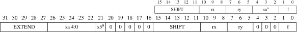
MIPS16 Regular and Extended Shift Instructions
For example, the opcode for adding an immediate value of 1 to r2 is 0x4a01. (r2 is the register for both the first argument to a function and its return value.) Because MIPS16 only encodes room for five immediate bits in this instruction, it allows for an extension word before the opcode to include extra bits. These can of course be zero, so 0xF000 0x4a01 also means addi r2, 1.
Some combinations are illegal. For example, extending the immediate bits of a NOP isn’t quite meaningful, so trying to execute 0xF008 0x6500 (Extended Immediate NOP) will trigger a bus error and the process will crash.
The Extended Shift instruction shown along with a regular Shift on page 337. Now how the prefix word changes the meaning of the subsequent instruction word.
However, thinking of these two words as a single instruction isn’t quite right, as we’ll soon see.
Delay Slots
Unlike ARM and Thumb, but like MIPS32 and SPARC, MIPS16 has a branch delay slot. The way most folks think of this, and the way that it is first explained by Patterson and Hennessy,3 is that the very next instruction after a branch is executed regardless of whether the branch is taken.
Sometimes this is hidden by an assembler, but a disassembler will usually show the instructions in their physical order. IDA Pro helpfully groups the delay-slot instruction into the proper block, so in graph view you won’t mistake it for being conditionally executed.
Extended Instructions in a Delay Slot
So what happens if we put a multi-word instruction into the delay slot? IDA Pro, being first written for X86, assumes that X86 rules apply and the whole chunk is one instruction. Qemu agrees, and a quick test of the following code reveals that the full instruction is executed in the delay slot.
We can test this as we see that on both real hardware and Qemu, extending an instruction like a NOP that shouldn’t be extended will trigger a bus error. However, when we put this combination after a return, it will only crash Qemu. In this case in hardware, only the extension word was fetched, which didn’t cause an issue.
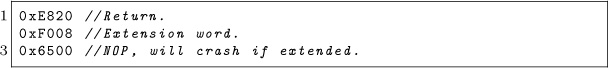
This is a known issue with the MIPS16e instruction set.4 To quote page 30, “There is only one restriction on the location of extensible instructions: They may not be placed in jump delay slots. Doing so causes UNPREDICTABLE results.”

Making Something Useful
We can now crash an emulator while allowing hardware to execute, but let’s improve this technique into something that can be used effectively for evasion. We’ll replace the NOP which caused the crash when extended with an instruction which is intended to be extended, specifically an add immediate, addi.

If we take that shellcode and view the IDA disassembly for it, you will see that, as above, IDA groups the delay-slot instruction into the function block so it looks like one is added to the return value. Take a look at this example, being careful to remember that $v0 means r2.
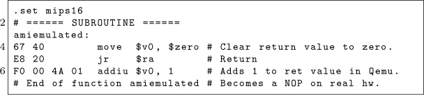
But hang on a minute, that delay slot holds two instruction words, and as we learned earlier, these can be thought of as separate instructions!
In fact, IDA only shows the instruction bytes on the left if you explicitly request a number of bytes from the assembly be shown. Without these being shown, a reverse engineer might forget that the program assembled a double-length instruction and thus that this behavior will occur.
This shows how we can confuse static analysis tools, which disassemble without taking into account this special case. Page 341 uses this handy shellcode to check for emulation.
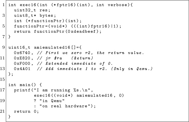
MIPS16 Function to Detect Qemu Emulation
We’ve discussed how IDA sees the extended addition as a single instruction, when in fact they are two separate MIPS instructions. But how is this handled in an emulator, as opposed to real MIPS hardware?
On the real hardware, when the return instruction is processed, the next instruction in the pipeline is 0xF000 (the extension instruction) and this is executed in the branch delay slot. That instruction, however, becomes a NOP in hardware.

The reason this detection works, we hypothesize, is because Qemu doesn’t actually have a pipeline, and thus it is emulated by knowing that it should run the instruction following a branch, to “correctly” handle the branch-delay slot. When it reads that next instruction, it reads the two instructions that it sees as a single extended instruction, instead of just reading the extension.
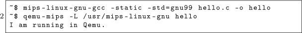
In hardware, we should note, the instruction isn’t exactly tossed away because it’s broken in half. The extension word, as the first half of the pair, never really gets executed on its own; rather, it hangs around in the pipeline to modify the subsequent instruction word. As the pipeline flows, the first word becomes a bubble as the second word becomes the single, unified instruction, but that unified instruction is too late to be executed. Instead, it is cruelly flushed from the MIPS16 pipeline while the bible ahead of it becomes a worthless NOP.
Thus, with just the eight byte function 0x6740 0xe820 0xf000 0x4a01, we can reliably detect emulation of MIPS16. As an added bonus, IDA Pro will agree with the simulation behavior, rather than the hardware’s behavior.
Kind thanks are due to Thorsten Haas for lending us a MIPS shell account on impossibly short notice. If you’d like to play around with more differences between hardware and emulation, we’ll note that in MIPS32, 0x03E00008 0x03E00008 is a clean return to $ra on hardware, but crashes Qemu. To crash on hardware and return normally in Qemu, use 0x03e0f809 0x8fe2-0001.
Cheers from Hanover, New Hampshire,
Travis and Ryan
15:10 Windows Kernel Race Condition Analysis While Accessing User-mode Data
by BSDaemon and NadavCh
In 2013, Google’s researchers Mateusz Jurczyk (J00ru) and Gynvael Coldwind released a paper entitled “Identifying and Exploiting Windows Kernel Race Conditions via Memory Access Patterns.”0 They discussed race conditions in the Windows kernel while accessing user-mode data and demonstrate how to find such conditions using an instrumented emulator. More importantly, they offered a very thorough explanation of how the identification of such issues is possible, specifically listing these conditions of interest:
- At least two reads of the same virtual address;
- Both read operations take place within a short time frame. The authors specifically recommend identifying reads in the handling of a single kernel entrance;
- The reads must execute in kernel mode;
- The virtual address subject to multiple reads must reside in memory writable by Ring-3 threads, in order for the user mode to be able to take advantage of the race.
Interestingly most of these races are exploitable—that is to say, possible for the attacker to win—on modern machines given multiple CPU cores. The exceptions would be in memory areas that are administrator-owned, or in situations that are early boot—and thus not in a memory area that can be mapped by an attacker. Even if the user-mode area is only writable by administrator-owned tasks, it might still be a problem given that it leads to code execution in kernel mode that is prohibited to the administrator and bypasses kernel driver signing. Notably, the early boot cases are only non-exploitable if they are not part of services prohibited after boot.
We reproduced Google’s research using Intel’s SAE1 and got some interesting results. This paper explains our approach in the hope of helping others understand the importance of documenting findings and processes. It also demonstrates other findings and clarifies the threat model for the Windows Kernel, thanks to our discussions with the MSRC. We share all the traces that generated double fetches for Windows 8 (pre and post booting) and Windows 10 (again, pre and post boot).2
We also share our implementation: it contains the parameters we used for our findings, the tracer, and the analyzer—and can be used as reference to audit other areas of the system. It also serves as a good way to understand the instrumentation capabilities of Simics and SAE, even though these are, unfortunately, not open-source tools.
For the findings per se, almost all parameters appear to be probed and copied to local buffers inside of try-except blocks. We flagged them as double-fetches because some of the pointers are probed first and then accessed to copy out actual data, like PUNICODE_STRING->Buffer. One of them is not inside a try-catch block and is a local DoS, but we do not consider it a security issue, since it is in administrator-owned memory. Many of them are not related to Unicode strings and are potential escalations-of-privilege (see Figure 15.16), but once again, for the threat model of the Windows Kernel, administrator-initiated attacks are out of scope.
Microsoft nevertheless fixed some of the reported issues. Obviously, mitigations in kernel mode might still prevent or make exploiting some of those very difficult.
Our findings concern three classes of issues:
Admin ↔ kernel cases: Microsoft did fix these, even though their threat model does not consider this a security issue. They may have considered the possibility of these cases used for a CSP bypass or a sandbox bypass—even though we did not find cases where a sandboxed process had administrator privileges.
Local DoS cases: These were also fixed, considering that a sym-link can be created by anyone and this was a non-admin-only case.
Other cases: The rest of the cases do not appear to be of consequence of security. We are sharing the traces with the community, in case anyone is interested in double-checking. :)
Tool Description
We implemented a Kernel Double Fetch tool (KDF), similar to the tool described in Identifying and Exploiting Windows Kernel Race Conditions via Memory Access Patterns.3 The tool has a runtime phase, in which KDF candidates are identified, and a post-runtime phase, in which these KDF candidates are analyzed based on whether the fetches are actually used by the kernel.
In the runtime phase, there is a ztool that looks for system-call related instructions. When such an instruction is triggered, the tool will dynamically configure itself to enable memory access notifications and instruction execution notifications. Whenever the kernel reads from the same user-space address twice or more, the tool will generate a file that describes the assembly instructions and the memory access addresses. As an optimization, the tool analyzes each system call number only the first time it is called; consecutive calls to the same system call will not be analyzed. As correctly pointed out by J00ru, though, this optimization can hinder the discovery of some potential bugs that are only reached under very specific conditions—and not during the first invocation of the affected system call. The code can be easily changed to address that concern.
After this work has completed, the KDF candidates are filtered, and only if the kernel read the memory twice or more and performed some operation based on the read, a violation will be reported.
We make the KDF ztool source code public. You may get it from under <zsim-kit>/src/ztools and open the Visual Studio solution. Make sure you build an x64 version of the tool. (Look in the Visual Studio configuration.) After that you can load the tool when you boot Win10. The tool generates candidates for KDF in separate log file in the current working directory. After completing the run of the simulation you may use the kdf_analyzer. The real KDF candidates will be located in the results directory.
cd src / ztools / kdf
python3.4 kdf_analyzer -id <zsim - simics - workspace >
-if <kdf - violations - basename > -rd < results - directory >
Approach
The simulation tool is dependent on SAE, and runs as a plugin to it. It works by loading the KDF tool included in this paper, booting the OS, and executing whatever test bench; the plugin will capture suspicious violations. After stopping the simulation, the KDF-analyzer scans the suspected violations recorded by the plugin and outputs the confirmed cases of double-fetches. Note that while these are real double-fetches, they are not necessarily security issues.
The algorithm of the plugin works as follows. It starts the analysis upon a syscall instruction, monitoring kernel reads from user addresses. It reports a violation on two reads from the same user-space address in the same instruction window. It stops the KDF analysis after Instruction-Window is reached in the same syscall scope, or upon a ring transition.
Performance is guaranteed since each syscall is instrumented only once and the instrumentation is enabled only in the system call range, supported by the tool itself.
The analyzer—responsible for post-analysis of the potential violations—is a Python script that manages the data flow dependencies. It adds a reference upon a copy from a suspected address to a register/address. It removes the dependency reference upon a write to a previously referenced register/memory, similar to a taint analysis. It reports a violation only if two or more distinct kernel reads happen from the same user-mode address.
We looked into the system call range 0–5081. We dynamically executed 450 syscalls within that range—meaning that our test bed is far from completely covering the entire range. The number of suspected cases flagged by the plugin was 67 and the number of violations identified was 8.
Interesting Cases
Figure 15.16 shows some of the interesting cases. The Windows version was build number 10240, TH1 RTM candidate.
You will find traces extracted from our tests in directories win10_after_boot/ and win8_after_boot/. As the names imply, they were collected after booting the respective Windows versions by just using the system: opening calc, notepad, and the recycle bin.
The filenames include the system call number and the address of the occurrence, to help identify the repeated cases, e.g., kdf-syscall-4101.log.data_flow_0x7ffe0320, kdf-syscall--4104.log.data_flow_0x7ffe0320, kdf-syscall-4105.log.-data_flow_0x7ffe0320. For example, the address 0x7ffe0320 repeats in both Win10 and Win8 traces. We kept these repeated traces just to facilitate the analysis.
We also include the directories results_win10_boot/ and results_win8_boot/, which show the traces of interest during the boot process. These conditions are less likely to be exploitable, but some addresses in them repeat post-boot as well.
The format of trace files is quite straightforward, with comments inserted for events of interest:
-- START ANALYZING KDF , ADDRESS : 0 x2f7406f390
-- -> Defines the address of interest
Also included are the instructions performed during the analysis/trace:
180: 0xfffff803650acdd4
mov rcx , qword ptr [rbx+0x10]
READ: VA = 0x2f7406f390, LA = 0 x2f7406f390,
PA1 = 0x79644390, SIZE = 0x8,
DATA = 0 x0002f746f3f8

Figure 15.16: Interesting cases.
The KDF detection happens on the following commentary on the trace:
-- Data - flow dependency originated from
-- line 180 is used : rcx
As you can see, the commentary includes the line at which the data-flow dependency was marked.
Our detection process begins when a syscall instruction is issued. While inside the call, we analyze kernel reads from the user address space, and report whenever two reads hit the same address; however, we remove references if a write is issued to the address. We stop the analysis once an instruction threshold is hit, or a ring transition happens.

Future Work
Leveraging our method and the toolset should make the following tasks possible.
First, it should be possible to find multiple writes to the same user-mode memory area in the scope of a single system service. This is effectively the opposite of the current concept of a violation. This may potentially find instances of accidentally disclosed sensitive data, such as uninitialized pool bytes, for a short while, before such data is replaced with the actual system call result.
Second, it should be possible to trace execution of code with CPL=0 from user-mode virtual address space, a condition otherwise detected by the SMEP mechanism introduced in the latest Intel processors. Similarly, it should be possible to trace execution of code from non-executable memory regions that are not subject to Data-Execution-Prevention, such as non-paged pools in Windows.
Third, KDF should be studied on more operating systems.
Last but not least, other cases of cross-privilege mode double fetches should be investigated. There is far more work left to be done in tracing access to find these sorts of bugs.
Acknowledgments
We would like to thank Google researchers Mateusz Jurczyk and Gynvael Coldwind for releasing an awesome paper on the subject with enough details to reproduce their findings. (Mateusz was also kind enough to give feedback on this paper.) MSRC for helping to better define the threat model for Windows Kernel Vulnerabilities, and for their collaboration to triage the issues. We also thank Intel’s Windows OS Team, specially Deepak Gupta and Volodymyr Pikhur, for their help in the analysis of the artifacts.

15:11 X86 is Turing-Complete without Data Fetches
by Chris Domas
One might expect that to compute, we must first somehow access data. Even the most primitive Turing tarpits generally provide some type of load and store operation. It may come as a surprise, then, that most modern architectures are Turing-complete without reading data at all!
We begin with the (somewhat uninspiring) observation that the effect of any traditional data fetch can be accomplished with a pure instruction fetch instead.
data:
.dword 0xdeadc0de
mov eax, [data]
That fetch in pure code would be a move sourced from an immediate value.
mov eax, 0xdeadc0de
With this, let us then model memory as an array of “fetch cells,” which load data through instruction fetches alone.
cell_0:
mov eax, 0xdeadc0de
jmp esi
cell_1:
mov eax, 0xfeedface
jmp esi
cell_2:
mov eax, 0xcafed00d
jmp esi
So to read a memory cell, without a data fetch, we’ll jmp to these cells after saving a return address. By using a jmp, rather than a traditional function call, we can avoid the indirect data fetches from the stack that occur during a ret.
mov esi, mret load return address
jmp cell_2 load cell 2
mret: return
A data write, then, could simply modify the immediate used in the read instruction.
mov [cell_1+1], 0xc0ffee set cell 1
Of course, for a proof of concept, we should actually compute something, without reading data. As is typical in this situation, the BrainFuck language is an ideal candidate for implementation— our fetch cells can be easily adapted to fit the BF memory model.
Reads from the BF memory space are performed through a jmp to the BF data cell, which loads an immediate, and jumps back. Writes to the BF memory space are executed as self modifying code, overwriting the immediate value loaded by the data cell. To satisfy our “no data fetch” requirement, we should implement the BrainFuck interpreter without a stack. The I/O BF instructions (. and ,), which use an int 0x80, will, at some point, use data reads of course, but this is merely a result of the Linux implementation of I/O.
First, let us create some macros to help with the simulated data fetches:
%macro simcall 1 %macro simwrite 2
mov esi, %%retsim mov edi, %2
jmp %1 shl edi, 3
%%retsim: add edi, %1+1
%endmacro mov [edi], eax
%%retsim:
%macro simfetch 2 %endmacro
mov edi, %2
shl edi, 3
add edi, %1
mov esi, %%retsim
jmp edi
%%retsim:
%endmacro
Next, we’ll compose the skeleton of a basic BF interpreter:
_start: je .decrement_dp
.execute: cmp al, ’+’
simcall fetch_ip je .increment_data
simfetch program, eax cmp al, ’-’
je .decrement_data
cmp al, 0 cmp al, ’[’
je .exit je .forward
cmp al, ’>’ cmp al, ’]’
je .increment_dp je .backward
cmp al, ’<’ jmp done

Then, we’ll implement each BF instruction without data fetches.
.increment_dp:
simcall fetch_dp
inc eax .forward.seek:
mov [dp], eax simcall fetch_ip
jmp .done inc eax
mov [ip], eax
simfetch program, eax
cmp al, ’]’
.decrement_dp: je .forward.seek.dec
simcall fetch_dp cmp al, ’[’
dec eax je .forward.seek.inc
mov [dp], eax jmp .forward.seek
jmp .done .forward.seek.inc:
inc ecx
jmp .forward.seek
.forward.seek.dec:
dec ecx
.increment_data: cmp ecx, 0
simcall fetch_dp je .done
mov edx, eax jmp .forward.seek
simfetch data, edx
inc eax
simwrite data, edx
jmp .done
.backward:
simcall fetch_dp
.decrement_data: simfetch data, eax
simcall fetch_dp cmp al, 0
mov edx, eax je .done
simfetch data, edx mov ecx, 1
dec eax .backward.seek:
simwrite data, edx simcall fetch_ip
jmp .done dec eax
mov [ip], eax
simfetch program, eax
cmp al, ’[’
.forward: je .backward.seek.dec
simcall fetch_dp cmp al, ’]’
simfetch data, eax je .backward.seek.inc
cmp al, 0 jmp backward.seek
jne .done
mov ecx, 1
.backward.seek.inc: .done:
inc ecx simcall fetch_ip
jmp .backward.seek inc eax
.backward.seek.dec: mov [ip], eax
dec ecx jmp .execute
cmp ecx, 0 .exit:
je .done mov eax, 1
jmp .backward.seek mov ebx, 0
int 0x80
Finally, let us construct the unusual memory tape and system state. In its data-fetchless form, it looks like this.
fetch_ip:
db 0xb8 mov eax, xxxxxxxx
ip:
dd 0
jmp esi
fetch_dp:
db 0xb8 mov eax, xxxxxxxx
dp:
dd 0
jmp esi
data:
times 30000
db 0xb8, 0, 0, 0, mov eax, xxxxxxxx, jmp esi, nop
0, 0xff, 0xe6, 0x90
program:
times 30000
db 0xb8, 0, 0, 0, mov eax, xxxxxxxx, jmp esi, nop
0, 0xff, 0xe6, 0x90
For brevity, we’ve omitted the I/O functionality from this description, but the complete interpreter source code is available.0
And behold! a functioning Turing machine on x86, capable of execution without ever touching the data read pipeline. Practical applications are nonexistent.
15:12 Nail in the Java Key Store Coffin
by Tobias “Floyd” Ospelt
The Java Key Store (JKS) is Java’s way of storing one or several cryptographic private and public keys for asymmetric cryptography in a file. While there are various key store formats, Java and Android still default to the JKS file format. JKS is one of the file formats for Java key stores, but the same acronym is confusingly also used the general key store API. This article explains the security mechanisms of the JKS file format and how the password protection of the private key can be cracked. Due to the unusual design of JKS, we can ignore the key store password and crack the private key password directly.
By exploiting a weakness of the Password Based Encryption scheme for the private key in JKS, passwords can be cracked very efficiently. As no public tool was available exploiting this weakness, we implemented this technique in Hashcat to amplify the efficiency of the algorithm with higher cracking speeds on GPUs.
The JKS File Format
Examples and API documentation for developers use the JKS file format heavily, without any security warnings. This format has been the default key store since key stores were introduced to Java. As early as 1999, JDK 1.2 introduced the “much stronger” JCEKS format that uses 3DES.0 However, JKS remained the default format. Just to mention some examples, Oracle databases and the Apache Tomcat webserver still use the JKS format to store their private keys.

When building an Android 7 app in the Android Studio IDE, it will create a JKS file with which to self-sign the app. Every application on Android needs to be signed before it can be installed on a device, and the phone will check that an update for an app is signed with the same key again. The private keys generated by Android Studio are valid for 25 years by default. Android does not offer any recovery mechanism to recover a lost private key, so efficient cracking of JKS files also benefits developers who forgot their passwords.
The JKS format is due to be replaced by PKCS12 as the default key store format in the upcoming Java 9.1 When talking to members of the security community who can still remember the nineties, some seem to remember that JKS uses some kind of weak cryptography, but nobody remembers exactly. Let’s explore weaknesses of the JKS file format and what an attacker needs to extract a private key in cleartext.
When a new key store is created and a new keypair generated, the developer has to set at least two passwords. There is not only a password for the key store as a whole (key store password), but each private key in it has its own password as well (private key password), while public keys do not have passwords. Both passwords are used independently. Surprisingly, the key store password is not used to encrypt any parts of the JKS file format, it is only used for integrity protection. This means the encrypted private key bytes and the cleartext bytes of public keys in a key store can be extracted without knowing the key store password.2 The password of the private key however, is used to apply a custom Password Based Encryption to the private key. Having two passwords leads to three possible cases.
In the first case, there is a password on the key store, but no private key password is used. (In practice, the available Java APIs prevent this.) However, in such a key store the private key would not be protected at all.
The second case is when the key store password and the private key password are identical. This is very common in practice and the default behavior of most tools such as Java’s keytool command. If no separate password for the private key is specified, the private key password will be set to the key store password.
In the third case, both passwords are set but the key store password is not the same as the private key password. While not the default behavior, it is still very common that users choose a different password for the private key.
It is important to demonstrate that in the third case some password crackers will crack a password that is useless and cannot be used to access the private key. The Jumbo version of the John the Ripper password cracking tool does this, cracking the (useless) key store password rather than the private key password. Let’s generate a key store with different key store (storepass) and private key password (keypass), then crack it with John:
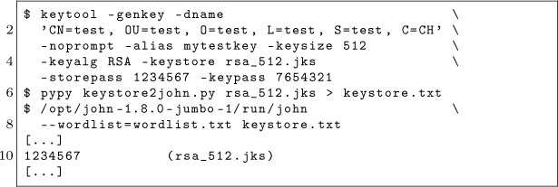
While this reveals the storepass, we cannot access the private key with this password. My proof of concept will crack the private key password instead:3

Naive Password Cracking
If we take the perspective of an attacker, we can conclude that we will not need to crack any password in the first case to get access to the private key. In theory, it also doesn’t matter which password we find out in the second case, as both are the same. And in the third case we can simply ignore the key store password; we only need to crack attack the private key password.
However, when we encounter the second case in practice, we would like to use the most efficient password cracking technique to find the key store password or the private key password. This means we need to explore first how each password can be cracked individually and which one leads to the most efficient cracking method.
There are already several programs that will try to crack the password of the key store:
- John the Ripper (JtR) Jumbo version4 extracts necessary information with a Python script and the cracking is implemented in C;
- KeyStoreBrute5 tries to load the key store via the official Java method in Java;
- KeystoreCracker6 uses the simple official Java way in Java as well;
- keystoreBrute7 uses keytool on the command line with the storepass option (subprocess);
- bruteforcer.py8 uses keytool on the command line with the storepass option (subprocess);
- Patator9 uses keytool on the command line with the store-pass option (subprocess).
All these parse the JKS file format first, which has a SHA-1 checksum at the end. They then calculate a SHA-1 hash consisting of the password, the magic “Mighty![]() Aphrodite” and all bytes of the key store file except for the checksum If the newly calculated hash matches the checksum, it was the correct password.
Aphrodite” and all bytes of the key store file except for the checksum If the newly calculated hash matches the checksum, it was the correct password.
No other operation with the key store password takes place when parsing the JKS file format; therefore, we can conclude that this password is only used for integrity protection. When the correct password is guessed and it is the same as the private key password, an attacker can now decrypt the private key.
From a performance perspective, this means that for every potential password a SHA-1 hash needs to be calculated of nearly all bytes of the key store file. As key stores usually hold private and public keys of at least 512-byte length, the SHA-1 hash is calculated over several thousand bytes of input. To summarize, the effort to check one password for validity is roughly:
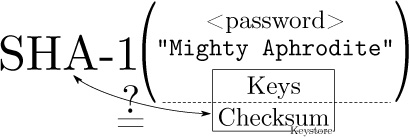
It is also important to emphasize again that these implementations will waste CPU time if the key store password is not identical to the private key password (third case) and are not attempting to crack the password necessary to extract the private key.
_____________
There are also implementations that crack the password of the private key directly:
- android-keystore-recovery10 tries to decrypt the entire private key with each password, in Scala;
- android-keystore-password-recover11 tries to decrypt the entire private key with each password, in Java.
These implementations have in common that they parse the JKS file format, but then only extract the entry of the encrypted private keys. For each private key entry, the first 20 bytes serve as an Initialization Vector and the last 20 bytes are again a checksum. The implementations then calculate a keystream. The keystream starts as the SHA-1 hash of the password plus IV. For every 20 bytes of the encrypted private key, the next 20 bytes of the keystream are calculated as the SHA-1 of the password plus previous keystream block (of 20 bytes). The encrypted private key bytes are then XORed with the keystream to get the private key in cleartext. This is a custom Password Based Encryption (PBE) scheme with chaining. As a last step, the cleartext private key is SHA-1 hashed again and compared to the checksum that was extracted from the JKS private key entry. Therefore, the effort to check one password for validity is roughly:
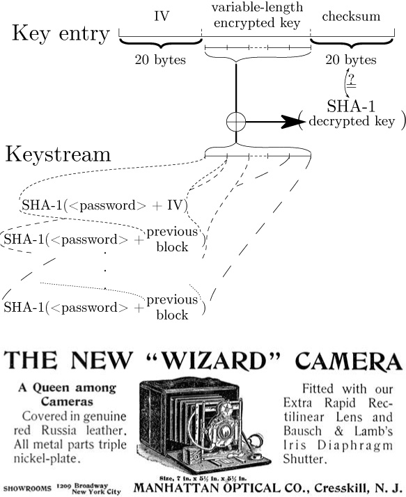
Efficient Password Cracking
From a naive perspective, it was not analyzed which of these algorithms would be more efficient for password cracking.12 However, an article on Cryptosense.com was published in 2016 and didn’t seem to get the attention it deserves.13 It points out that for the private key password cracking method it is not necessary to calculate the entire keystream to reject an invalid password. As the cleartext private key will be a DER encoded file format, the first SHA-1 calculation of password plus IV with the XOR operation is sufficient to check if a password candidate could potentially lead to a valid DER encoded private key. These all miss out on this optimization and therefore do too many SHA-1 calculations for every password candidate.
It turns out, it is even possible to pre-calculate the XOR operation. For each password candidate only one SHA-1 hash needs to be calculated, then some bytes of the result have to be compared to the pre-calculated bytes. If the bytes are identical, this proves that the password might decrypt the key to a DER format. Practical tests showed that a DER encoded RSA private key in cleartext will start with 0x30 and bytes at index six to nineteen will be 0x00300d06092a864886f70d010101. Similar fingerprints exist for DSA and EC keys. These bytes we expect in a DER encoded private key can be XORed with the corresponding encrypted private key bytes to precalculate the SHA-1 output bytes we are looking for.
This means, the cracking can be optimized to use a more efficient two-step cracking algorithm to crack the private key password. After parsing the JKS file format and precalculating the necessary values, we have the following optimized algorithm:
0. Choose a password in pseudo UTF-16, meaning that a null byte is added to every character.
1. keystream = SHA-1(password + STATIC_20_BYTES_IV_-FROM_PRIVKEY_ENTRY)
2. Check if bytes at index 0 and 6 to 19 of the keystream correspond to PRECOMPUTED_15_BYTES_DER_PROOF. If they are not the same, go to step 0.
3. Let keybytes be every 20 bytes of STATIC_VARIABLE_-LEN_ENCRYPTED_BYTES_FROM_PRIVKEY_ENTRY.
4. For each keybytes:
a) key += keystream ⊕ keybytes
b) keystream = SHA-1(password∥keystream)
5. checksum = SHA-1(password∥key)
6. Check if checksum is STATIC_20_BYTES_CHECKSUM_FROM_-PRIVKEY_ENTRY. If they are the same, key is the private key in cleartext and we can stop. Otherwise, go to step 0.
As practical tests will later indicate, step 3 is typically never reached with an incorrect password during cracking and all passwords can be rejected early. In fact, Hashcat only implements steps 0 to 3, as the probability that a wrong candidate is ever found is neglectible (1/2120)!
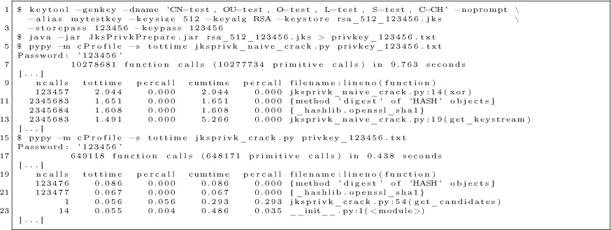
Figure 15.17: Java Key Store with a Short Password
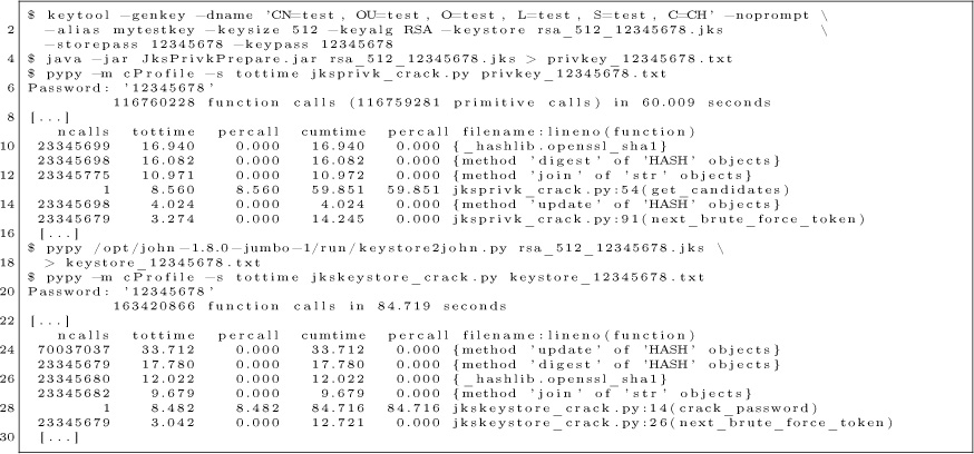
Figure 15.18: Java Key Store with a Longer Password
Implementation
The parsing of the file format and extraction of the precomputed values for cracking were implemented as a standalone JAR Java version 8 command line application JksPrivkPrepare.jar. The script will prepare the precomputed values for a given JKS file and outputs it as asterix separated values.
As a PoC, a Python script jksprivk_crack.py14 was implemented to do the actual cracking of the private key password. To put a final nail in the coffin of the JKS format, it is important to enable the security community to do efficient password cracking.15 To optimize cracking speed, Jens “atom” Steube— developer of the Hashcat password recovery program— implemented the cracking step in GPU optimized code. Hashcat takes the same arguments as the Python cracking script. As hashcat uses a weakness in SHA-1,16 the cracking speed on a single NVidia GTX 1080 GPU reaches around 7.8 (stock clock) to 8.5 (overclocked) billion password tries per second.17 This allows to try all alphanumeric passwords (uppercase, lowercase, numbers) of length eight in about eight hours on a single GPU.

Benchmarking
When doing a benchmark, it is important to try to measure the actual algorithm and not some inefficiency of the implementation. Some simple measurements were done by implementing the described techniques in Python. All the mentioned resources are available in the feelies.18 Let’s first look at the naive implementation of the private key cracker jksprivk_naive_crack.py versus the efficient private key cracking algorithm jksprivk_crack.py. Let’s generate a test JKS file first. We can generate a small 512-byte RSA key pair with the password 123456, then crack it with both implementations. Both implementations only try numeric passwords, starting with length 6 password 000000 and incrementing, as in Figure 15.17.
These measurements show that a lot more calls to the update and digest function of SHA-1 are necessary to crack the password in the naive script. If the keysize of the private key in the JKS store is bigger, the time difference is even greater. Therefore, we conclude that our efficient cracking method is far more suitable.
Now we still have to compare the efficient cracking of the private key password with the cracking of the key store password. The algorithm for key store password cracking was also implemented in Python: jkskeystore_crack.py. It takes a password file as argument like John the Ripper does. As these implementations are more efficient, let’s generate a new JKS with a longer password, as shown in Figure 15.18.
In this profile, we see that the update method of the SHA-1 object when cracking the key store takes much longer to return and is called more often, as more data goes into the SHA-1 calculation. Again, the efficient cracking algorithm for the private key is faster and the difference is even bigger for bigger key sizes.
So far we tried to compare techniques in Python. As they use the same SHA-1 implementation, the benchmarking was kind of fair. Let’s compare two vastly different implementations, the efficient algorithm jksprivk_crack.py to John the Ripper. First, create a wordlist for John with the same numeric passwords as the Python script will try, then run the comparison shown in Figure 15.19.
That figure shows that John is faster for 512-bit keys, but as soon as we grow to 1024-bit keys in Figure 15.20, we see that our humble little Python script wins the race against John. It’s faster, even without John’s fancy C code or optimizations!
As John the Ripper needs to do SHA-1 operations for the entire key store content, the Python script outperforms John the Ripper. For larger key sizes, the difference is even bigger.
These benchmarks were all done with CPU calculations and Hashcat will use performance optimized GPU code and Markov Chains for password generation. Cracking a JKS with private key password POC||GTFO on a single overclocked NVidia GTX 1080 GPU is illustrated on Figure 15.21.
Neighborly greetings go out to atom, vollkorn, cem, doegox, ange, xonox and rexploit for supporting this article in one form or another.![]()

Figure 15.19: John 1.8.0-jumbo-1 is faster for 512-byte keystores.
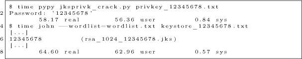
Figure 15.20: For 1024-bit keystores, our script is faster.

Figure 15.21: Cracking session on a NVidia GTX 1080 GPU.

15:13 The Gamma Trick: Two PNGs for the price of one
by Hector ‘Marcan’ Martin
Say you’re browsing your favorite hypertext-encoded, bitmap-containing visuo-lingual information distribution medium. You come across an image which—as we do not yet live in an era of infinitely scalable resolution—piques your interest yet is presented as a small thumbnail. Why are they called thumbnails, anyway?
Despite the clear instructions not to do so, you resolve to click, tap, press enter, or otherwise engage with the image. After all, you have been conditioned to expect that such an action will yield a higher-quality image through some opaque and clearly incomprehensible process.
Yet the image now appearing before your eyes is not the same image that you clicked on. Curses! What is this sorcery? Have I been fooled? Is this alien technology? Did someone hack Reddit?
The first time I came across this technique was a few years ago on a post on 4chan. Despite the fact that the image was not just lewd but downright unsavory to my taste, I have to admit I spent quite some time analysing exactly what was going on in detail. I have since seen this trick used a few times here and there, and indeed I’ve even used a variant of it myself in a CTF challenge. Thanks go to my friend @Miluda for giving me permission to use her art in this article’s examples.

So, do tell, what is going on? It all has to do with the PNG format. Like most image formats, PNG images carry metadata. That metadata includes information about how the image, and in particular color information, is itself encoded. The PNG format can specify how RGB values map to how much light comes out of the pixels on your screen in several ways, but one of the simplest is the ‘gAMA’ chunk which specifies the gamma value of the image, γ.
Intuitively, you’d think that a pixel with 50% brightness would be encoded as a 0.5 value (or about 0x7f, in an 8-bit format), but that is not the case. Due to a series of historical circumstances and practical coincidences too long-winded to be worth going into, pixel brightness values are not linear. Instead, they are stored as the brightness value raised to a power γ. The most common default is γ = 0. 4545. When the image is displayed, the pixels are raised to the inverse gamma, 2.2, to obtain the linear brightness value.0 This is typically done by your monitor. Thus, 50% brightness is actually encoded as 0. 73, or 0xba. PNG images can specify an alternate γ value, and your PNG decoder is responsible for converting it to the correct display gamma.
Like every other optional feature of every other file format, whether this is actually implemented is anyone’s guess. As it turns out, most web browsers implement it properly, and most image processing libraries do not. Many websites use these to create thumbnails: Reddit, 4chan, Imgur, Google Docs. We can use this to our advantage.
Take one source image and darken it by mapping its brightness range to 0%.. 80%. Take the other source image, and lighten it by mapping its brightness range to 80%.. 100%. The two images now occupy distinct portions of the brightness gamut. Now, for every 2 × 2 group of pixels, take 3 pixels of the darker image and 1 pixel of the lighter image. Finally, encode the result as a PNG and apply the gAMA PNG tag, using an extreme value such as γ = 0.0227. (Twenty times lower than the default γ = 0.4545.)
We can do this easily enough with ImageMagick:

When viewed without the specified gamma correction, all of the lighter pixels (25% of the image) approach white and the overall image looks like a washed out version of the darker source image (75% of the image). The 2 × 2 pixel pattern disappears when the image is downscaled to less than half of its original dimensions (if the scaler is any good anyway). When the gamma correction is applied to the original image, however, all the darker pixels are crushed to black, and now the lighter pixels span most of the brightness spectrum, revealing the lighter image as a grid of bright pixels against a black background. If the image is displayed at 1:1 pixel scale, it will look quite clean. Scales between 100% and 50% typically result in moiré artifacts, because most scalers cheat. Scaling down usually darkens the image, because most scalers also don’t do gamma-correct scaling.1

This approach is the one I’ve seen used so far, and it is easy to achieve using the Levels tool in GIMP, but we can do better. The second image is much too dark: we’re mapping the image to a linear brightness range, but then applying a very much non-linear gamma correction. Also, in the first image, we can see a “halo” of the second image, since the information is actually there. We can fix these issues.
Let’s use ImageMagick again. First we’ll apply a true gamma adjustment to the high source image. The -gamma operation in ImageMagick performs an adjustment by the inverse of the supplied value, so to apply an adjustment of γ = 1/20 we’ll pass in 20. We’ll also slightly increase its brightness, to ensure that after gamma adjustment the pixels are close enough to white:

This effectively maps the image range to 0.0350.05 = 0.846.. 1.0, but with a non-linear gamma curve. Next, because the low image will appear washed out, we’ll apply a gamma of 0. 8, then darken it to 77% of its original brightness. 0.7720 = 0.005, which is dark enough to not be noticeable. We’re keeping this in a variable to chain later.
$ low_gamma =" - alpha off - gamma 0.8 + level 0% ,77% "
Now let’s compensate for the halo caused by the high image. For every 2 × 2 output pixels, we’d like an average color of:
υ = 3/4υlow + 1/4
That is, as if the high image was completely white. What we actually have is:
Solving for ![]() gives:
gives:
The -compose Mathematics flag of ImageMagick allows us to implement this.

There will be some slight edge effects, due to aliasing issues between the chosen pixels from both images, but this will remove any blatant solid halo areas. This correction assumes that the thumbnail scaler does not perform gamma-correct scaling, which is the common case. This means it is incorrect if the output image is viewed at 1:1 scale (the halo will be visible), but once scaled down it will disappear. In order to cater for gamma-correct scalers (or 1:1 viewing), we’d have to perform the adjustment in a linear colorspace.
Finally, we just compose both images together with a pattern as before:
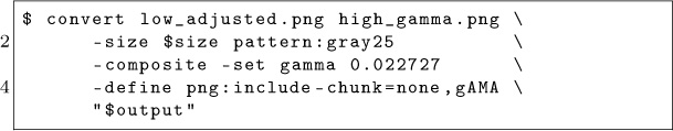

The result is much better!


The previous images in this article have been filtered (2 × 2 box blur) to remove the high-frequency pixel pattern, in order to approximate how they would visually appear in a browser context without relying on the specific scaling/resampling behavior of your PDF renderer. In fact, the filtering method varies: gamma-naive for simulating thumbnailing, gamma-aware for simulating the true response at 1:1 scale. For your amusement, here are the raw images. Their appearance will depend on exactly what kind of filtering, scaling, or other processing is applied when the PDF is rasterized. Feel free to play with your zoom setting.
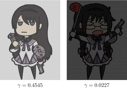
Yup, it’s 2017 and most software still can’t up/downscale images properly. Now don’t get me started on the bane that is non-premultiplied alpha, but that’s a topic for another day.![]()