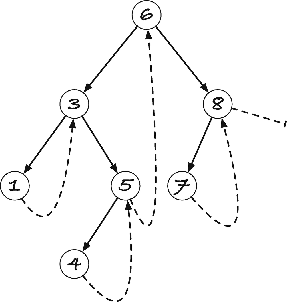
Search trees , or in this chapter specifically binary search trees, are also recursively defined. A binary search tree is either an empty tree or a node containing a value and two trees, a left and a right subtree. Furthermore, we require that the value in a node is larger than all the values in its left subtree and smaller than all the values in its right subtree. It is the last property that makes search trees interesting for many algorithms. If we know that the smaller values are to the left, and the larger values are to the right, we can efficiently search in a tree, as we shall see.

Three different search trees containing the numbers 1, 3, 6, and 8
The time this search takes is proportional to the height of the tree, which can be proportional to the number of elements the tree holds (as is the case in the trees in A) and C) in Figure 12-1). If the tree is balanced, so the depth of the left and right subtrees is roughly the same for all the nodes, then the depth is logarithmic in the number of elements. There are many strategies for keeping a search tree balanced, but I will refer you to a textbook on algorithms and data structures to explore that. In this chapter, we will only look at strategies for implementing the data structure. For simplicity, we will only consider trees that hold integers and without duplications.
Tree Operations
- 1.
Determine if a value is in a tree
- 2.
Insert a new element in a tree
- 3.
Delete a value from a tree
and of course we should have code for freeing a tree once we are done with it.
Contains
- 1.
If t is empty, we report that v is not in it.
- 2.
If the value in t is v, then we report that it is.
- 3.
Otherwise, if v is smaller than the value in t, we look in t’s left subtree, and if it is larger, we look in t’s right subtree.
It is a recursive operation, where we have two base cases: t is empty or it holds the value we are looking for. The recursive case involves searching a subtree, where we can determine which subtree to search from the value in the root of t.
Insert
- 1.
If t is empty, we should create a tree with a single leaf, a node that holds the value v and has empty left and right subtrees.
- 2.
If t has a value, and it is v, then we leave t as it is. It already has the value, and the order property from the definition prevents a search tree from holding more than one of the same value.
- 3.
Otherwise, if v is smaller than the value in t, insert it into t’s left subtree, and if v is greater, insert it into t’s right subtree.
Again, we have a recursive operation. The base cases are again an empty tree or a tree with v in its root, and the recursive cases are insertions into the left or right subtree.
Delete
- 1.
If t is empty, we are done.
- 2.
If t’s value is v, then delete t and replace it with a subtree (see the following).
- 3.
Otherwise, delete v from the left or right subtree, depending on whether v is smaller than or greater than the value in v.
Step 2 is where the operation is more complicated than the others. To delete the value in the root of a tree, we need to construct a tree that still has all the remaining values. There are two cases here. One, when t has at most one non-empty subtree, we can immediately replace it, and two, if both its subtrees are non-empty, we replace the value in t with the largest value in its left subtree and then remove that value from the left subtree.
Consider case one, where t has at least one empty subtree, and consider Figure 12-2. In the figure, t is the tree rooted in the black node, and the gray triangle represents the (possible) non-empty tree. If we replace t with its non-empty subtree, we have deleted the value, since any value appears at most once in a tree. All values in t’s subtree are smaller than the value in t’s parent, if t is a left subtree, or greater than the value in t’s parent, if t is a right subtree. So replacing t with its subtree will satisfy the order property of search trees.

Deleting in a tree with at most one non-empty subtree

Deleting a value in a tree with two non-empty subtrees
The procedure works just as well by getting the leftmost value in the right subtree, but we chose the rightmost in the left more by tradition than anything else.
Free
- 1.
To free an empty tree, do nothing—it is already freed.
- 2.
Otherwise, free the left and the right subtree, and then free the tree.
Recursive Data Structures and Recursive Functions
We didn’t talk about it when we implemented lists because lists are particularly simple to work with. Still, when it comes to recursive data structures, it is often useful to think about operations on them as well in terms of recursion. Recursive solutions are usually much more straightforward than corresponding iterative solutions, as they closely match the data structure. However, they come at a cost. If we solve a problem recursively, the recursive calls can fill the call stack, which will crash our program, if we are lucky, or corrupt our memory. With search trees, this is usually not an issue. If we keep a search tree balanced, then the recursion depth is logarithmic in the number of nodes in the tree. That means that we can double the number of nodes and only have to go one recursive call deeper. Unfortunately, we are not writing balanced trees in this chapter, so that will do us no good. And even if we did have balanced trees, there is some overhead in function calls that we can avoid if we do not use recursion.
So, what can we do when the best solution, from a programming perspective, is clean recursive code, but where execution constraints prevent us from recursion? We will explore this with the operations we need on trees in this chapter, but the short answer is that, sometimes, recursion isn’t a problem, and you can safely use recursive functions. This is the case with so-called tail recursion. If a function calls itself but immediately returns the result of the recursive call—so it doesn’t do any further processing with the result of the recursive call, it just returns it—the function is said to be tail-recursive. Then recursion isn’t necessary at all. Most compilers, if you turn on optimization, will translate such functions into loops, and calling them involves a single stack frame only. You do not risk filling the stack, and you do not get any function call overhead beyond the first call. If your compiler doesn’t do this for you, it is also trivial to rewrite such a function yourself. We will see several examples of such recursions.
We cannot always get tail-recursive solutions.1 In a tree, if we need to recurse on both subtrees of a node, for example, to free memory, then at most one of the recursive calls can be the result of the function itself. When you are in this situation, you might have to allocate an explicit stack on the heap. There is more available memory on the heap than on the stack, so this alleviates the problem with exceeding the stack space. It isn’t always trivial to replace a call stack with an explicit stack, however. Call stacks do more than pushing new calls on the stack; when you are done with a recursive call, you also need to return to the correct position in the calling function. You must emulate function calls in your own code, and while sometimes easy, it can get complicated. We will see a few examples of using explicit stacks and discuss why it isn’t advisable in the cases where we need them for our trees.
If we consider using an explicit stack for something like freeing the nodes in a tree, there is another issue. If the stack requires that we allocate heap memory—which it must, if we should be able to handle arbitrarily large trees—then the operation can fail. Should malloc() return NULL, we have an error. We have to deal with that, but if we need the memory to complete the recursive tree traversal, then we are in trouble. Something like freeing memory should never fail—must never fail—because it is practically impossible to recover from. And even if we can recover from a failure, we likely will leak memory. It is far better to have a solution where we can reuse memory we already have to solve the problem. There is, of course, not a general solution for this. What memory we might be able to reuse and how we can arrange existing memory depend on the data structure we have. There is usually a solution if you work at it a little bit. We will see a way to modify search trees that lets us traverse and delete trees without using recursion, an explicit stack, or any additional memory.
There is much to cover, so read on.
Direct Implementation
We start by implementing a direct translation of the operations into C. It will have some issues, in particular with error handling and efficiency, but we will soon fix those.
There is no particular good reason to prefer one version over the other; I just happen to like the first one.
This is a good solution for that operation, and there is nothing I would change about it. It is simple, it follows the definition of the operation directly, and it is tail-recursive. In the two recursive cases, the return value of contains() is the direct result of the recursive calls to contains(). This means that likely your compiler will translate the recursive calls into a loop in the generated code. If you are not afraid to look at assembler code, you can check the generated code using, for example, godbolt.org, where I have put this function at the link https://godbolt.org/z/3adTr3. There, you can see what different compilers will generate for this function. If you generate code without optimization, the recursive functions will have one or more 'call' instructions in them. If you turn on optimization, that call disappears and you have loops (in various forms, depending on the compiler). Godbolt.org is an excellent resource if you want to know what code your compiler is generating. To check if a tail-recursive function is translated into a loop, you can generally check if it generates code with a call instruction or not. If your compiler isn’t supported by godbolt.org, you will have to generate the assembler yourself—the compiler’s documentation will tell you how—and then you can check. Compilers generally translate tail-recursive functions into loops. The C standard doesn’t require it, but it is usually a safe assumption.
We return a new leaf with the value if t is empty. If val is smaller than t->value, update t’s left subtree with an insertion, and if it is greater, we update t’s right subtree with an insertion. If t->value == val, we don’t do anything; we just return t at the end of the function.
This function is more problematic than contains(). First, we might have an allocation error in leaf(), in which case we return an empty tree that shouldn’t be empty. This is easy to capture if we start out with an empty tree since we will probably notice that adding a value to an empty tree shouldn’t give us an empty tree back. However, if we insert into a non-empty tree, we call recursively down the tree structure, and somewhere down there, we insert an empty subtree that should have been a leaf. We do not get any information about that back from the call. We get a pointer to the input tree back regardless of whether there was an error or not.
Of course, if the value is already in the tree, we have allocated a new node for no reason, but that is the cost of handling allocation errors correctly here. Upfront allocation, even if you risk deleting again, is often an acceptable solution to problems such as these. If you want to avoid an extra allocation, you can always call contains() first (at the cost of an extra search).
Another issue is that the function is not tail-recursive. When we insert val in a subtree, we need to update one of t’s subtrees accordingly. When we have more work to do after a recursive call, we cannot get tail recursion. Consequently, there will be function calls here, with the overhead they incur and the risk of exceeding the stack space.
We will not call it with an empty tree, so we assert that. Otherwise, t->right would be dereferencing a NULL pointer, which we always want to avoid. We test if there is a right subtree, and if there isn’t, we return t’s value. Otherwise, we continue searching in t’s right subtree. The function is tail-recursive, and with an optimizing compiler, you get an efficient looping function.
will give us the left subtree if it isn’t empty and otherwise give us the right subtree. If both trees are empty, we get the right subtree, but that doesn’t matter, since they are both NULL. If t has both subtrees, we get the rightmost value, put it in t->value, and then we delete it from t->left.
Finally, if t->value is greater or smaller than val, we delete recursively, updating the left or right subtree accordingly.
This function, like insert(), is not tail-recursive. Updating the subtrees after the recursive calls prevents this.
This, obviously, isn’t tail-recursive either. We cannot make it tail-recursive because there are two recursive calls involved.
We don’t have recursion issues here, at least not directly. We iteratively call insert() (which does have recursion issues).
Pass by Reference
The problems we have with insertion and deletion are caused by the same design flaw we had in the first list implementation in Chapter 11. We have designed the functions such that they return a new tree instead of modifying an existing one. That means that the recursive calls give us the trees we now need to store in one of t’s subtrees. The changes we made to lists will also work here. We want the functions to take a tree that we can update as input. That means that an empty tree cannot be a NULL pointer, but must be something else, or at least that if it is a NULL pointer, it is passed by reference. We can use either of the solutions from the lists, make a pointer to pointers our representation, or use a dummy node. The first solution will work for us here, so that is what we will do.
We will still have the type stree be a pointer to struct node, but change the operations, so they work with pointers to stree instead of stree. So the functions take pointers to pointers to nodes. An empty tree is a pointer to a NULL pointer.
It allocates an stree * pointer and, if successful, sets the pointed-to value to NULL, making it an empty tree.
To make the code more readable, I cast *tp to an stree so I can refer to the tree with the variable t. Little else changes in the function, but in the recursive calls we must provide an address of a tree, not the tree itself. So, we get the address of t’s left or right subtree when we call contains() recursively. We need to call contains() with an address of a struct node pointer, so we call recursively with &t->left (the address of left subtree) or &t->right (the address of the right subtree). The & operator binds such that &t->left means &(t->left), the address of t’s left member, not (&t)->left, which would be the left member of whatever structure the address of t is. Since &t isn’t a pointer to a structure, it is a pointer to a pointer, and it hasn’t got a left member, the expression (&t)->left would give you a type error.
We, once again, get the tree that target points to, to make the code more readable. If it is NULL, then target is an address that holds an empty tree, and we want that address to hold a new leaf instead. We, therefore, allocate a leaf and put it in *target. An assignment is also an expression, so (*target = leaf(val)) gives us a value. It is the right-hand side of the assignment, which is the new leaf. If the allocation failed, we get NULL. If we turn a pointer into a truth value (with the !! trick we have seen before), then we turn the assignment into a value that is true if the allocation was successful and false otherwise, which we will return to indicate whether the insertion was successful or not.
The recursive cases didn’t change, except that we pass the address of the subtrees along in the call, instead of just the subtrees. That means that we can modify the tree we use in the recursion, so we don’t need to update the tree after the call. The function is now tail-recursive.
Be careful when you use an address as a parameter to a function call. You can get into trouble if it is the address of a stack object. There is nothing wrong with it per se. If we put a tree (an stree object) on the stack, and use it with our operations, then we have a tree on the stack, and as long as we do not use it after we have returned (which we can’t as it is gone by then), then all is well. But if we, for example, took the address of t and passed it along in a recursive call in insert(), we could write into the address, but we would be writing into a local variable. What we put there is lost once the call to insert() is done. Also, the compiler would see that we use the address of a local variable that presumably should change in recursive calls where we get new memory for local variables, so the tail recursion optimization would not be possible. That, though, is a minor problem, since the function would be broken already if we attempt to pass addresses of local variables along in the call. It is not what we do here, of course. The addresses we pass along in the function calls are addresses in heap-allocated nodes.
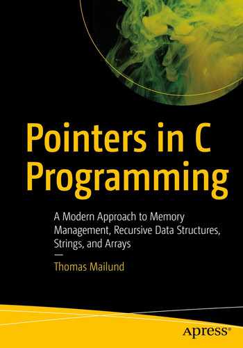
Return value of rightmost()
Our new rightmost() returns the address that holds the pointer to the rightmost tree; see Figure 12-4. We search down a tree’s right trees until we get to a node where right is empty. However, the variable we use in the function is the address that holds the tree, not the tree itself. So, when we reach the rightmost node, the parameter to the rightmost() call is the address in the parent node. Dereferencing the result of the rightmost() call gives us the rightmost node, and writing into the result changes the right tree in the parent. We exploit this to delete the rightmost value from the left tree. We dereference the rightmost reference to put the value into t, and then we replace the rightmost tree with its left child directly, no second call to delete() this time.
In print_stree(), I didn’t bother with a variable that holds the dereferenced value of the parameter. Here, t is the pointer to a tree. That means that I need to dereference t to get a tree, which is why you see expressions such as &(*t)->left. We dereference t to get a tree, *t, then get the left tree in that, (*t)->left, and then we get the address of that tree, &(*t)->left.
Refactoring
Iterative Functions
The contains(), insert(), and delete() operations are no longer recursive, but they rely on find_loc() and rightmost() that are. Both of those, however, are tail-recursive, so the code that the compiler generates, when you enable optimization, will not involve function calls. Of course, if you are not comfortable relying on the mercy of your compiler’s optimization, you can translate the functions into iterative ones yourself. With tail-recursive functions, that is usually straightforward.
Explicit Stacks
Free and print still use recursion. If we want to avoid exceeding the stack space, we can move the recursion from the call stack to an explicit stack. We shall see that it carries its own problems, but let us implement it first.
The push() and pop() functions take the stack by reference, a pointer to a pointer to a stack frame, so they can modify the stack. When we push(), we allocate a new stack frame, initialize it with a node and the top of the stack, and then we point the stack to the new frame so the new frame is now the top of the stack. If the allocation fails, we terminate the program. Freeing data should never fail because we don’t know how to handle such a situation—we are probably leaving the program in an inconsistent state, and we will most likely leak memory. We could attempt to recover, so we don’t crash the entire program, but here I give up and call abort(). In the following printing code, we will recover slightly more gracefully.
When we push the left child first, we process it last, since stacks work in a first-in, first-out fashion. If we wanted to process the left tree first, as we do in the recursion, we would have to push the subtrees in the opposite order. It doesn’t matter when we are deleting the nodes, though, so deleting right subtrees before left subtrees is fine.
The stack is a pointer to a frame as well, but I will also put a jmp_buf to handle allocation errors. This is a buffer in which we can store the program’s state, which in practice means its registers. If we call the function setjmp(), we store the registers. If we later call longjmp(), we restore them. Restoring means that we reset the stack and instruction pointers, so the program goes to the position on the stack where we called setjmp(), and the instruction pointer starts executing right after the call to setjmp(). The only difference between the call to setjmp() when we stored the registers and when/if we returned to it from a longjmp() is that setjmp() returns zero the first time and a value we give to longjmp() the second time.
The setjmp()/longjmp() functions are a crude version of raising and catching exceptions. We can return to an arbitrary point on the stack, with the program’s registers restored, but there is no checking for whether it is a valid state. You can call longjmp() with registers that moves you to a stack frame that is long gone. The mechanism does nothing to clean up resources, and if you lose pointers to heap-allocated memory in a jump, then it is gone. You need to be careful to free resources when you use this mechanism, just as you must be with normal returns from functions. It is highly unsafe, but it will work for our purposes here. We get a way to return to our printing function from nested function calls that push to the stack.
An allocation failure results in a longjmp() which we will catch in the main function. The second argument to longjmp(), here 1, is what setjmp() will have returned in the restored state. As long as it is not zero, we can recognize that we have returned from a longjmp(). We won’t implement a pop() operation because we will deal with popping directly in the printing function.
If we get an allocation error, then the push function will call longjmp(), which results in us returning from setjmp() a second time, but now with a non-zero return value. If that happens, we goto the error label and free the stack. In the while-loop, we must free top before we call handle_print_op(). We might not return from handle_print_op—the longjmp() error handling will send us directly to the setjmp()—so we must leave the function in a state where the code in error can clean up all resources. If we free top before we handle the operation, all the stack frames are on the stack, and the error handling code will free them.
Here, we can handle an error, but we cannot undo the damage we have done by writing parts of the tree to output and then bailing. What we print, we cannot undo. And when we use an explicit stack, we can get allocation errors we will have to recover from (unless we give up and abort, as with free_nodes()). There are many cases where we need to dynamically allocate memory for stacks and queues and whatnot when our programs run, but for freeing memory, or for operations that we cannot undo, we should try hard to avoid allocations. This isn’t always possible, but for traversing trees, there are tricks.
For more complex recursions, though, a node must hold all the information necessary for that algorithm, so the structure can grow in complexity beyond what we are willing to accept.
Morris Traversal
Many algorithms can traverse a tree without using an implicit or explicit stack, and we will see one in this section. This algorithm, Morris traversal, doesn’t require that we add any additional data to the nodes. Instead, it uses a clever way to modify the tree as we traverse it, to simulate recursion, and then restores it to its initial state as the simulated traversal returns.
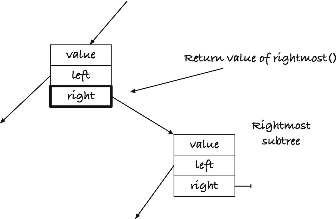
A (right) threaded tree
Imagine that we need to do an in-order traversal of such a tree. We can recurse by following left pointers as long as we have them, which in the example will take us to node 1. Here, we cannot continue further left, so we visit 1 (we have, trivially, visited all its left children). Now we recurse to the right, that is, we follow its right pointer. Node 1 doesn’t have a right child, but we have a “threaded” pointer instead that works like one, so going right from 1 corresponds to returning from the recursion to node 3. When we enter node 3, we would have to recurse to the right, unless we can recognize that we had already been there, so let us, for now, assume that we tag the nodes so we can tell that we have already been to node 3 once. If we can see that, we know that we came back from a left recursion, so we visit node 3 and recurse to the right. In 5, a node we haven’t seen before, we recurse to the left, and we get to node 4, where we cannot go further left. We visit 4 and go right. That takes us back to 5, where we realize that we have been before, so we go right instead of left this time, which takes us up to 6. Recognizing that we have been here before, we go right instead of left, to 8, and recurse from here. We have not been here, so we go left, to 7. We cannot continue left, so we go right, back to 8. Since we have been in 8 once before, we visit the node, and then we go right. This time, there is no right child, threaded or otherwise, so the traversal ends.
If we have a threaded tree, the “recursion” works as follows: If we have a node we haven’t seen before, we go left. If we have a node that we have seen before, we visit it and go right. “Returning” from the recursion happens whenever a step to the right is along a threaded pointer rather than a real subtree.
How can we get the threaded pointers, and how can we recognize that we are in a node that we have seen before? Notice that if you have a node “n”, and another node, m, has a threaded pointer to it, then n is the next value after m in the tree. That means that m is the rightmost node in n’s subtree. So we can go from n to m with our rightmost() function . Once there, we can, of course, write a pointer to n into the right subtree. So when we enter a node the first time, we can run down and find the node where we should insert a threaded pointer. How do we recognize that we have visited a node before? If we search for the rightmost node in the left subtree, and we encounter the node itself, then we have inserted it the first time we visited the node! So the same rightmost search will tell us if we are seeing a node for the first time or for the second time.
The rightmost() macro is there, so we can use rightmost() in deletion, without the weird extra argument.
If you don’t have a left subtree, you visit the node and go right. Otherwise, you figure out if you can find yourself as the rightmost node on the left. If not, you update the rightmost node’s right subtree to point to the current node, and you recurse to the left. If yes, you restore the right subtree in the rightmost node by setting it to NULL, you visit the current node, and then you go right.
The running time is proportional to the size of the tree. You search for the rightmost node in the left subtree twice in every node (that has a left subtree), but the nodes you run through in such searches do not overlap between different nodes, so each node is maximally visited twice in such searches.
You don’t quite get the recursion in print_stree() here, although you visit the nodes in the same order. It is simple to output the left parentheses, the commas, and the node values, but when you return from the recursion by going through a right pointer, you go up a number of recursive calls in one step, and you can’t see how many. You can annotate the nodes with depth information and get print_stree() behavior, but I will not bother here. Traversing the nodes in order suffices for most applications, and we rarely need to know the exact tree structure.
Freeing Nodes Without Recursion and Memory Allocation
It simplifies the algorithm, and we save one rightmost search per node. And we free the tree without using any additional memory, so freeing cannot fail due to stack exhaustion, due to recession, or due to memory allocation errors, if we had used an explicit stack.
Adding a Parent Pointer
A problem with both embedding a stack in the nodes and with Morris traversal is that we can at most run one traversal at a time—because we are using shared memory embedded in the trees. With Morris traversal, we must also complete the traversal before the tree is restored to a consistent state (with the embedded stack, it isn’t a problem as we overwrite the stack in a new traversal). Concurrency is out of the question with these strategies (and with many related strategies that rely on modifying trees for traversal).
If we are willing to add a pointer to the parent of each node (with NULL in the root), then we can traverse a tree without modifying it and without dynamically allocating memory while we do it. This does mean extending the node struct, of course, but for many of the strategies for balancing trees, a parent pointer is necessary in any case, or at least makes the code vastly faster, so it is not a high price to pay.
You can avoid the checks for empty children, before you set the parent pointer, by having a dummy node for empty trees. You can share the same node with all empty trees because you will never need to take the parent of an empty tree. You will just need to replace the tests for NULL empty trees with tests for whether a tree points to the dummy.
There are plenty more algorithms for traversing trees, with or without modifying them, and if you want to get more experience with trees and pointer manipulation, it is a good place to start. For the book, however, it is time to move on to the next topic.