
3 Modelling of multi-conductor overhead lines and cables
3.1 General
In this chapter, we present the modelling of multi-conductor overhead lines and cables both in the phase and sequence frames of reference. Calculations and measurement techniques of the electrical parameters, or constants, of lines and cables are described. Transposition analysis of single-circuit and multiple-circuit overhead lines, and sheaths and cores of cables are presented as well as their π models in the sequence and phase frames of reference.
3.2 Phase and sequence modelling of three-phase overhead lines
3.2.1 Background
The transmission and distribution of three-phase electrical power on overhead lines requires the use of at least three-phase conductors. Most low voltage lines use three-phase conductors forming a single three-phase circuit. Many higher voltage lines consist of a single three-phase circuit or two three-phase circuits strung or suspended from the same tower structure and usually called a double-circuit line. The two circuits may be strung in a variety of configurations such as vertical, horizontal or triangular configurations. Figure 3.1 illustrates typical single-circuit lines and double-circuit lines in horizontal, triangular and vertical phase conductor arrangements. A line may also consist of two circuits running physically in parallel but on different towers. In addition, a few lines have been built with three, four or even six three-phase circuits strung on the same tower structure in various horizontal and/or triangular formations. In England and Wales, almost 99% of the 400 kV and 275 kV overhead transmission system consists of vertical or near vertical double-circuit line configurations.

Figure 3.1 (a) Typical single-circuit and double-circuit overhead lines and (b) double-circuit overhead lines with one earth wire: twin bundle = 2 conductors per phase and quad bundle = 4 conductors per phase
In addition to the phase conductors, earth wire conductors may be strung to the tower top and normally bonded to the top of the earthed tower. Earth wires perform two important functions; shielding the phase conductors from direct lightning strikes and providing a low impedance path for the short-circuit fault current in the event of a back flashover from the phase conductors to the tower structure. The ground itself over which the line runs is an important additional lossy conductor having a complex and distributed electrical characteristics. In the case of high resistivity or lossy earths, it is usual to use a counterpoise, i.e. a wire buried underground beneath the tower base and connected to the footings of the towers. This serves to reduce the effective tower footing resistance. Where a metallic pipeline runs in close proximity to an overhead line, a counterpoise may also be used in parallel with the pipeline in order to reduce the induced voltage on the pipeline from the power line.
Therefore, a practical overhead transmission line is a complex arrangement of conductors all of which are mutually coupled not only to each other but also to earth. The mutual coupling is both electromagnetic (i.e. inductive) and electrostatic (i.e. capacitive). The asymmetrical positions of the phase conductors with respect to each other, the earth wire(s) and/or the surface of the earth cause some unbalance in the phase impedances, and hence currents and voltages. This is undesirable and in order to minimise the effect of line unbalance, it is possible to interchange the conductor positions at regular intervals along the line route, a practice known as transposition. The aim of this is to achieve some averaging of line parameters and hence balance for each phase. However, in practice, and in order to avoid the inconvenience, costs and delays, most lines are not transposed along their routes but transposition is carried out where it is physically convenient at the line terminals, i.e. at substations.
Bundled phase conductors are usually used on transmission lines at 220 kV and above. These are constructed with more than one conductor per phase separated at regular intervals along the span length between two towers by metal spacers. Conductor bundles of two, three, four, six and eight are in use in various countries and in Great Britain, two, three (triangle) and four (square or rectangle) conductor bundles are used at 275 and 400 kV. The purpose of bundled conductors is to reduce the voltage gradients at the surface of the conductors because the bundle appears as an equivalent conductor of much larger diameter than that of the component conductors. This minimises active losses due to corona, reduces noise generation, e.g. radio interference, reduces the inductive reactance and increases the capacitive susceptance or capacitance of the line. The latter two effects improve the steady state power transfer capability of the line. Figure 3.1(a)(ii) shows a typical 400 kV double-circuit line of vertical phase conductor arrangement having four bundled conductors per phase, one earth wire and one counterpoise wire. The total number of conductors in such a multi-conductor system is (4 × 3) × 2 + 1 + 1 = 26 conductors, all of which are mutually coupled to each other and to earth.
3.2.2 Overview of the calculation of overhead line parameters
General
A line is a static power plant that has electrical parameters distributed along its length. The basic parameters of the line are conductor series impedance and shunt admittance. Each conductor has a self-impedance and there is a mutual impedance between any two conductors. The impedance generally consists of a resistance and a reactance. The shunt admittance consists of the conductor’s conductance to ground and the susceptance between conductors and between each conductor and earth. The conductance of the air path to earth represents the leakage current along the line insulators due to corona. This is negligibly small and is normally ignored in short circuit, power flow and transient stability analysis.
Practical calculations of multi-conductor line parameters with series impedance expressed in pu length (e.g. ω/km) and shunt susceptance in μS/km are carried out using digital computer programs. These parameters are then used to form the line series impedance and shunt admittance matrices in the phase frame of reference as will be described later. The line capacitances or susceptances are calculated from the line potential coefficients which are essentially dependent on the line and tower physical dimensions and geometry. The calculations use the method of image conductors, assumes that the earth is a plane at a uniform zero potential and that the conductor radii are much smaller than the spacings among the conductors. The self and mutual impedances depend on the conductor material, construction, tower or line physical dimensions or geometry, and on the earth’s resistivity. Figure 3.2 is a general illustration of overhead line tower physical dimensions and spacings of conductors above the earth’s surface as well as conductor images below earth used for the calculation of line electrical parameters.

Figure 3.2 A general illustration of an overhead line physical dimensions and conductor spacings relative to tower centre and earth
The fundamental theories used in the calculations of resistance, inductance and capacitance parameters of overhead lines are extensively covered in most basic power system textbooks and will not be repeated here. Practical digital computer based calculations used in industry consider the effect of earth as a lossy conducting medium. The equations used in the calculation of line parameters are presented below.
Potential coefficients, shunt capacitances and susceptances
Using Figure 3.2, given a set of N conductors, the potential V of conductor i due to conductor’s own charge and charges on all other conductors is given by
 (3.1)
(3.1)where Pij is the Maxwell’s potential coefficient expressed in km/F and Qj is the charge in C/km. The equations assume an infinitely long perfectly horizontal conductors above earth whose effect is included using the method of electrostatic images. This method is generally valid up to a frequency of about 1 MHz. The potential of a conductor i above earth due to its own charge and an equal but negative charge on its own image enables us to calculate the self-potential coefficient of conductor i as follows:
where yi is the height of conductor i above earth in m and ri is the radius of conductor i in m. Clearly yi is much greater than ri. The potential of conductor i due to a charge on conductor j and an equal but negative charge on the image of conductor j enables us to calculate the mutual potential coefficient between conductor i and conductor j as follows:
where Dij is the distance between conductor i and the image beneath the earth’s surface of conductor j in m, and dij is the distance between conductor i and conductor j in m. Equation (3.1) can be rewritten in matrix form as
where P is a potential coefficient matrix of N × N dimension. Multiplying both sides of Equation (3.3a) by P−1, we obtain
C is line’s shunt capacitance matrix and is equal to the inverse of the potential coefficient matrix P. Under steady state conditions, the current and voltage vectors are phasors and are related by
since the line’s conductance is negligible at power frequency f. The line’s shunt susceptance matrix is given by
Series self and mutual impedances
Self impedance
The equations assume infinitely long and perfectly horizontal conductors above a homogeneous conducting earth having a uniform resistivity ρc(ωm) and a unit relative permeability. Proximity effect between conductors is neglected. Using Figure 3.2, the series voltage drop in V of each conductor due to current flowing in the conductor itself and currents flowing in all other conductors in the same direction is given by
 (3.5a)
where Z is the impedance expressed in Ω/km and I is the current in amps. The self-impedance of conductor i is given by
where subscript c represents the contribution of conductor i resistance and internal reactance, g represents a reactance contribution to conductor i due to its geometry, i.e. an external reactance contribution and e represents correction terms to conductor i resistance and reactance due to the contribution of the earth return path. If skin effect is neglected, i.e. assuming a direct current (dc) condition or zero frequency, the internal dc impedance of a solid magnetic round conductor, illustrated in Figure 3.3(a), is given by

Figure 3.3 Illustration of some conductor types: cross-section of a (a) solid round conductor, (b) tubular round conductor and (c) 30/7 stranded conductor (30 Aluminium, 7 inner steel stands)
where μr and ρc are the relative permeability and resistivity of the conductor, respectively, and rc is the conductor’s radius.
Where skin effect is to be taken into account, the following exact equation for the internal impedance of a solid round conductor can be used
is defined as the complex propagation constant and δ is skin depth or depth of penetration into the conductor and is given by
and Ii are modified Bessel functions of the first kind of order i. For calculation of line parameters close to power frequency, the following alternative equation, suitable for hand calculations using electronic calculators, is found accurate up to about 200 Hz:
Equation (3.8) shows that skin effect causes an increase in the conductor’s effective ac resistance and a decrease in its effective ac internal reactance. Also, at f = 0, Equation (3.8) reduces to Equation (3.6).
In the case of a tubular or hollow conductor, illustrated in Figure 3.3(b), the dc internal impedance is given by
 (3.9)
(3.9)Mathematically, the case of a solid round conductor is a special case of the hollow conductor since by setting ri = 0, Equation (3.9) reduces to Equation (3.6). Aluminium conductor steel reinforced (ACSR) or modern gapped-type conductors can be represented as hollow conductors if the effect of steel saturation can be ignored. Saturation may be caused by the flow of current through the helix formed by each Aluminium strand that produces a magnetic field within the steel.
Where skin effect of a hollow conductor is to be taken into account, the following exact equation for the internal impedance of such a conductor can be used
 (3.10a)
 (3.10b)
where Ii and Ki are modified Bessel functions of the first and second kind of order i, respectively. Mathematical solutions suitable for digital computations that provide sufficient accuracy are available in standard handbooks of mathematical functions and also in modern libraries of digital computer programs. Equation (3.7a) that represents the case of a solid conductor can be obtained from Equation (3.10a) by substituting ri = 0.
The external reactance of conductor i due to its geometry is given by
In practice, the internal reactance of a conductor is much smaller than its external reactance except in the case of very large conductors at high frequencies. Generally, precision improvements in the former would have very small effect on the total reactance.
The contribution of the earth’s correction terms to the self-impedance of conductor i is presented after the next section.
Earth return path impedances
The contributions of correction terms to the self and mutual impedances, due to the earth return path, are generally given as infinite series. The resistance and reactance general correction terms are calculated in terms of two parameters mij and θij as follows
 (3.13a)
 (3.13b)
 (3.14a)
 (3.14b)
and δ is the skin depth defined in Equation (3.7b). The coefficients used in Equation (3.13) are given by

The sign in bn alternates every four terms that is sign = +1 for n = 1, 2, 3, 4 then sign = -1 for n = 5, 6, 7, 8 and so on.
Various forms of Equation (3.13) can be given depending on the value of mij. For short-circuit, power flow and transient stability analysis, the line parameters are calculated at power frequency, i.e. 50 or 60 Hz. For such calculations, mij is normally less than unity and generally one term in the series would be sufficient to give good accuracy. At higher frequencies, two cases are distinguished; the first is for 1 < mij ≤ 5, where the full series is usually used whereas for mij > 5, the series converges to an asymptotic form and simple finite expressions that provide acceptable accuracy may be used provided that θij < 45°. Generally, the number of correction terms required increases with frequency if sufficient accuracy is to be maintained.
Using the skin depth δ of Equation (3.7b), and an earth relative permeability of unity, the effect of earth return path is defined as an equivalent conductor at a depth given by
Therefore, for the self-impedance, the resistance and reactance correction terms are given by
 (3.16a)
 (3.16b)
and for the mutual impedance, the correction terms are given by
 (3.17a)
 (3.17b)
Typical values of earth resistivity are: 1–20 ωm for garden and marshy soil, 10–100 ωm for loam and clay, 60–200 ωm for farmland, 250–500 ωm for sand, 300–1000 ωm for pebbles, 1000–10000 ωm for rock and 109 ωm for sandstone. Resistivity of sea water is typically 0.1–1 ωm. Using an average earth resistivity of a reasonably wet soil of 20 ωm, the depth of the equivalent earth return conductor Derc given in Equation (3.15) is equal to 416.7 m at 50 Hz and 380.4 m at 60 Hz.
Summary of self and mutual impedances
Substituting Equations (3.11), (3.16a) and (3.16b) in Equation (3.5), the self-impedance of conductor i with earth return is given by
 (3.18a)
Substituting Equations (3.12) and (3.17) in Equation (3.12), the mutual impedance between conductor i and conductor j with earth return is given by
 (3.18b)
For non-digital computer calculations of impedances at power frequency, e.g. using electronic hand calculators, the use of the first earth correction term for resistance and reactance is usually sufficient. Assuming that the power frequency inductance of a general tubular conductor does not appreciably reduce below its dc value given in Equation (3.9), Equation (3.18a) reduces to
 (3.19b)
For a non-magnetic solid conductor with μr = 1 and ri = 0, we obtain from Equation (3.19b), f(ro, ri) = 1 giving a value for the internal inductance in Equation (3.19a) of 1/4. Combining this with the logarithmic term, the latter changes to loge [Derc/(0.7788 × ro)] where 0.7788 × ro is known as the geometric mean radius of the conductor.
Similarly, combining its two logarithmic terms, Equation (3.18b) reduces to
When calculating mutual impedances between conductors of circuits that are separated by a distance d, Equation (3.20a) is generally sufficiently accurate for
For an earth resistivity of 20 ωm and f = 50 Hz, Derc = 416.7 m and dij ≤ 57 m.
Stranded conductors
Overhead lines with stranded conductors are extensively used and their effect is important in calculating power frequency line parameters. Figure 3.3(c) illustrates a conductor that consists of N strands. Even a tightly packed bundle of a large number of strands will still leave small unfilled gaps between the strands. The total cross-sectional area of the strands is smaller than the equivalent cross-sectional area of a solid conductor. This reduction factor is the area of the conductors divided by the area of the equivalent solid conductor and can be used to increase the equivalent conductor effective resistivity whilst keeping its overall radius the same. However, for line parameter calculations, the equivalent geometric mean radius of the conductor is calculated and for a general conductor that consists of N strands each having a radius r, this is given by
 (3.21)
The effect of stranding causes a reduction in the outer radius of the equivalent conductor of the bundle of strands. A reduction factor, termed the stranding factor, is defined as the ratio of the geometric mean radius, GMRc, of the conductor to the conductor’s outer radius and this can be calculated for any known stranding arrangement. For example, for a homogeneous conductor that consists of seven strands arranged on a hexagonal array, it can be shown that the area reduction factor is equal to 0.77778 and the stranding factor is equal to 0.72557.
Bundled phase conductors
Figure 3.4 illustrates a general case of a phase bundle consisting of N conductors per phase with asymmetrical spacings between the conductors. Practical examples of such asymmetrical arrangement are rectangular and non-equilateral triangular bundles. Asymmetrical conductor bundles of two or more conductors can be represented by an equivalent single conductor. The radius of the equivalent conductor can be calculated by applying the GMR technique to an arbitrary set of axes and origin as shown in Figure 3.4. The GMR of the equivalent conductor of the entire bundle is given by

 (3.22)
where N is ≥2 and is the number of conductors in the bundle. When impedance calculations are carried out, GMRc is the geometric mean radius of one conductor in the bundle. When potential coefficient calculations are carried out, GMRc is equal to the conductor’s outer radius.
Special cases of symmetrical conductor bundles are shown in Figure 3.5. This shows bundles of two, three, four and six conductors, with circles drawn through the centres of the individual conductors. It can be shown that the general Equation (3.22) of the equivalent GMREq reduces to

where A is the radius of a circle through the centres of the bundled conductors and is given by
and d is the spacing between any two adjacent conductors in the symmetrical bundle.
It should be noted that for N subconductors in a bundle, the internal resistance and inductance included in Equation (3.19a) must be divided by N.
An alternative method of bundling phase conductors is to form the full phase impedance and susceptance matrices from the parameters of all conductors including bundled subconductors and earth wires. For example, for a single-circuit line with one earth wire and four conductors per phase, the dimension of the resultant phase impedance matrix is 13 × 13. The bundled conductors are effectively short-circuited by zero impedance so the voltages are equal for all the subconductors in the bundle and the sum of currents in all subconductors is equal to the equivalent phase current. For example, for phase R, the subconductor voltages are V1 = V2 = V3 = V4 = VR whereas for the subconductor currents, I1 + I2 + I3 + I4 = IR. Using these voltage and current constraints, the bundle conductors can then be combined using standard matrix reduction techniques to produce a 4 × 4 matrix that represents three equivalent phase conductors and one earth wire.
Average height of conductor above earth
The calculation of line parameters is based on the assumption of perfectly horizontal conductors above the earth’s plane. The average sag of phase conductors and earth wires between towers together with the height of the conductor at the tower can be used to calculate an average conductor height for use in the calculation of line’s electrical parameters. Using Figure 3.6, it can be shown that the average height of the earth wire conductor above ground is given by

 (3.24)
where Ht is the conductor height at the tower in m and Sav is the average conductor sag in m measured at mid-span between two suspension towers and usually assumed to apply to the entire line length, i.e. ignoring the effect of angle or tension towers. For span lengths of up to 400 to 500 m, a simple formula can be derived by assuming that the variation of conductor height with distance between the two towers is a parabola, that is
where xms is half the span length. The average height above ground between the two towers is calculated by integrating Equation (3.25) over the span length, i.e.
The calculation of average conductor height should take into account the different sags of phase and earth wire conductors.
3.2.3 Untransposed single-circuit three-phase lines with and without earth wires
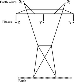
Consider a general case of a multi-conductor single-circuit three-phase overhead line with asymmetrical spacings between the conductors, two earth wires and with earth return as shown in Figure 3.7.
Phase and sequence series impedance matrices
Figure 3.8(a) shows the coupled series inductive circuit of Figure 3.7 where each phase and earth wire conductors, and earth are represented as equivalent self and mutually coupled impedances.

Figure 3.8 Series impedance and shunt susceptance circuits of Figure 3.7: (a) three-phase coupled series impedance circuit; (b) three-phase coupled shunt capacitance circuit; (c) reduced three-phase shunt capacitance circuit with earth wires eliminated and (d) three-phase shunt capacitance circuit in sequence terms
To derive a general formulation of the series phase impedance matrix for such a line, the phase R series impedance voltage drop equation can be written as
With the phases at the receiving end all earthed, IR + IY + IB = IE + IS1 + IS2 and using Equation (3.27b) in Equation (3.27a), we have

where
 (3.28b)
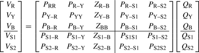
The self and mutual phase impedances defined in Equation (3.28b) as well as those of the earth wires include the effect of earth impedance ZEE. We can write similar equations for ΔVY, ΔVB, ΔVS1, ΔVS2 and combine them all to obtain the following series voltage drop and partitioned series phase impedance matrix:
 (3.29)
In large-scale power system short-circuit analysis, we are interested in the calculation of short-circuit currents on the faulted phases R, Y or B or a combination of these but generally not in the currents flowing in the earth wires. One exception is the calculation of earth fault return currents covered in Chapter 10. For the elimination of the earth wires, the partitioned Equation (3.29) is rewritten as follows:
 (3.30b)
ZAA consists of the self and mutual impedances of phase conductors R, Y and B with earth return. ZAS consists of the mutual impedances between the phase conductors R, Y and B, and earth wires S1 and S2, with earth return. ![]() noting that the individual impedances are symmetric, i.e. ZRS1-E = ZS1R-E. ZSS consists of the self and mutual impedances of the earth wires S1 and S2 with earth return. The earth return effect is shown in Equation (3.28b). Expanding Equation (3.30a), we obtain
noting that the individual impedances are symmetric, i.e. ZRS1-E = ZS1R-E. ZSS consists of the self and mutual impedances of the earth wires S1 and S2 with earth return. The earth return effect is shown in Equation (3.28b). Expanding Equation (3.30a), we obtain
In the majority of line installations, the earth wires are bonded to the tower tops and are only partially earthed by the footing resistance of each tower to which they are connected but solidly earthed at substations. However, it is usual to assume zero tower footing resistances and that the earth wires are at zero voltage at all points. Thus, using ΔVS1S2 = 0 in Equation (3.31b) and substituting the result in Equation (3.31a), we obtain
 (3.32c)
Equation (3.32b) shows that the self and mutual phase impedances of the phase conductors of matrix ZAA are reduced by the presence of the earth wires. Equation (3.32c) indicates the elements of the phase impedance matrix of the single-circuit three-phase line with both earth wires eliminated and including the effect of the earth impedance. It is noted that the mathematical elimination of the earth wires only eliminates their presence from the full matrix but not their effects which are included in the modified elements of the reduced matrix, i.e. ZRR(S-E) –; ZRR–E.
Although far less common, segmented earth wires may be used to prevent circulating currents in earth wires and associated I2R losses. This is a ‘T’ arrangement where the earth wires are bonded to the top of the middle tower but insulated at the adjacent towers on either side. This is equivalent to IS1 = IS2 = 0 in Equation (3.29) and hence the reduced phase impedance matrix ZRYB(S–E) is directly obtained from Equation (3.29) by deleting the last two rows and columns that correspond to the earth wires. This results in ZRYB(S–E) = ZAA. The impedance matrix of Equation (3.32c) is symmetric about the diagonal and in the case of asymmetrical spacings between the conductors, the self or diagonal terms are generally not equal to each other, and neither are the mutual or off-diagonal terms. Currents flowing in any one conductor will induce voltage drops in the other two conductors and these may be unequal even if the currents are balanced. This is because the mutual impedances, which are dependent on the physical spacings of the conductors, are unequal. Rewriting the voltage drop equation using Equation (3.32c) and dropping the S and E notation for convenience, we can write
 (3.33)
Assuming balanced three-phase currents, i.e. IY = h2IR and IB = hIR where h = ej2π/3, we obtain from Equation (3.33)
Equation (3.34) describes the per-phase or single-phase representation of the three-phase system when balanced currents flow. However, the three per-phase equivalent impedances are clearly unequal and a single per-phase representation cannot be used.
The sequence impedance matrix of the phase impedance matrix given in Equation (3.33) can be calculated, assuming a phase rotation of RYB, using VRYB = HVPNZ and IRYB = HIPNZ where H is the sequence to phase transformation matrix given in Chapter 2. Therefore,

where the nine sequence impedance elements of this matrix are as given by Equation (2.26a) in Chapter 2.
The conversion to the sequence reference frame still produces a full and even asymmetric sequence impedance matrix that includes intersequence mutual coupling. Where this intersequence coupling is to be eliminated, the circuit has to be perfectly transposed. Transposition is dealt with in Section 3.2.4.
Phase and sequence shunt susceptance matrices
Figure 3.8(b) shows the shunt capacitance circuit of Figure 3.7 involving phase conductors and earth. To derive the shunt phase susceptance matrix, we use the potential coefficients calculated from the line’s dimensions. Thus, the voltage on each conductor to ground as a function of the electric charges on all the conductors is given by
Again, with the earth wires at zero voltage, they are eliminated from Equation (3.36b) as follows
Again, PRYB(S) is the reduced potential coefficient matrix that includes the effects of the eliminated earth wires. Equation (3.37b) shows that the self and mutual potential coefficients of the phase conductors of the matrix PAA are reduced by the presence of the earth wires. To derive the shunt phase capacitance matrix of the line, multiplying Equation (3.37a) by ![]() , we obtain
, we obtain
and CRYB(S) is the shunt phase capacitance matrix.
Expanding Equation (3.38b), and noting that the capacitance matrix elements include the effect of the eliminated earth wires, we have
 (3.38c)
In Equation (3.38c), the elements of this capacitance matrix are increased by the presence of the earth wires which reduce the potential coefficients. Equation (3.38c) is illustrated in the reduced shunt capacitance equivalent shown in Figure 3.8(c) after the elimination of the earth wires but not their effects. Using Equations (3.4b) and (3.38c) and dropping the S notation for convenience, the nodal admittance matrix of Figure 3.8(c) is given by
 (3.39a)
The negative signs for the off-diagonal capacitance or susceptance terms are due to the matrices being in nodal form. For example, from Figure 3.8(c), and using susceptances instead of capacitances, the injected current into node R is given by
and similarly for IY and IB. The off-diagonal terms represent shunt susceptances between two-phase conductors, e.g. R and Y, etc. The diagonal terms, e.g. that for conductor R, represent the sum of the shunt capacitances between conductor R and all other conductors including earth as shown in Figure 3.8(c).
The shunt susceptance matrix of Equation (3.39a) is symmetric about the diagonal but in the case of asymmetrical spacings between the conductors, the self that is diagonal terms are generally not equal to each other, and neither are the mutual or off-diagonal terms. Therefore, as for the series phase impedance matrix, the sequence shunt susceptance matrix is given by

where the nine sequence susceptance elements of this matrix are as given by Equation (2.26b) in Chapter 2 but with Z replaced by B.
As for the series sequence impedance matrix, the intersequence mutual coupling present can be eliminated by assuming the line to be perfectly transposed. This is dealt with in the Section 3.2.4.
An alternative method to obtain the reduced 3 × 3 capacitance matrix of Equation (3.38c) is to calculate the inverse of the 5 × 5 potential coefficient matrix of Equation (3.36a) which gives a 5 × 5 shunt capacitance matrix. The 3 × 3 shunt capacitance matrix can then be directly obtained by simply deleting the last two rows and columns that correspond to the earth wires. The reader is encouraged to prove this statement.
We have presented in this section the general case of an untransposed single-circuit three-phase line with two earth wires. The cases where the line has only one earth wire or no earth wires become special cases from a mathematical viewpoint. The 5 × 5 matrices of Equations (3.29) and (3.36a) become 4 × 4 matrices in the case of one earth wire and 3 × 3 matrices in the case of no earth wires and the rest of the analysis is similar. If the earth wires are identical and are symmetrical with respect to the three-phase circuit, they can be initially analytically replaced by an equivalent single earth wire whose equivalent impedance is half the sum of the self-impedance of one earth wire and the mutual impedance between the earth wires. However, analytical calculations are not necessary because of the extensive use in industry of digital computer calculations of line parameters or constants.
3.2.4 Transposition of single-circuit three-phase lines
We have shown in Section 3.2.3 that the calculated sequence series impedance and shunt susceptance matrices include full intersequence mutual couplings. However, as presented in Chapter 2, sequence component reference frame analysis is based on separate positive phase sequence (PPS), negative phase sequence (NPS) and zero phase sequence (ZPS) circuits. To eliminate the intersequence mutual couplings, an assumption can be made that the line is perfectly transposed. The objective of transposition is to produce equal series self-impedances, and equal series mutual impedances in the phase frame of reference and similarly for the shunt self-susceptances and shunt mutual susceptances. Perfect phase transposition means that each phase conductor occupies successively the same physical positions as the other two conductors in two successive line sections as shown in Figure 3.9.

Figure 3.9 Transposition of a single-circuit three-phase line: (a) forward successive phase transpositions and (b) reverse successive phase transpositions
Figure 3.9 shows three sections of a transposed line. This represents a perfectly transposed line where the three sections have equal length. Perfect transposition results in the same total voltage drop for each phase conductor and hence equal average series self-impedances of each phase conductor. This effect also applies to the average series phase mutual impedances, average shunt phase self-susceptances and average shunt phase mutual susceptances. Figure 3.9(a) illustrates a complete forward transposition cycle, i.e. three transpositions where the line is divided into three sections and t, m and b are used to designate the conductor physical positions on the tower. If the three conductors of the circuit are designated C1, C2 and C3, then a forward transposition is defined as one where the conductor positions for the three sections are C1C2C3, C3C1C2 then C2C3C1 as shown in Figure 3.9(a).
Using Equation (3.33), the series voltage drops per-unit length across conductors C1, C2 and C3 for each section of the line can be calculated taking into account the changing positions of the three conductors on the tower and hence their changing impedances. With equal section lengths, i.e. l1 = l2 = l3 = ![]() , the voltage drops for each section of the line are given as
, the voltage drops for each section of the line are given as
 (3.42a)
 (3.42b)
 (3.42c)
where Z is a total impedance of the line. Therefore, the voltage drop across each conductor of the line is given by
 (3.43a)
 (3.43b)
ZPhase is the phase impedance matrix of the perfectly transposed line, noting that individual conductor impedances are symmetric.
We have shown how to calculate the phase impedance matrix for each line transposition section from first principles. However, a general matrix analysis approach is more suitable for modern calculations by digital computers. Let us define a transposition matrix that has the following characteristics:
 (3.44)
Using Equation (3.42) and noting the successive changing positions of the three conductors in Figure 3.9(a), Equation (3.42) can be rewritten as
 (3.45)
Using the transposition matrix defined in Equation (3.44), we can write for Section 2


Similarly for Section 3, we can write


In summary, the phase impedance matrices of the first, second and third line transposition sections are given by
 (3.48a)
and the phase impedance matrix of the perfectly transposed line is given by
This analysis approach is straightforward if the effect of the matrix T is recognised. The effect of pre-multiplying matrix ZSection-1 by matrix T is to shift its row 2 elements up to row 1, row 3 elements up to row 2 and row 1 elements to row 3. Also, the effect of post-multiplying matrix ZSection-1 by matrix Tt is to shift its column 2 elements to column 1, column 3 elements to column 2 and column 1 elements to column 3. A reverse successive transposition cycle could also be used to obtain the same result as illustrated in Figure 3.9(b). The reader is encouraged to show that the phase impedance matrix of each transposition section, using transposition matrix T, is given by
 (3.49a)
and the phase impedance is given by
Equation (3.43b) is the phase impedance matrix of our balanced or perfectly transposed single-circuit line. Assuming R, Y, B is the electrical phase rotation of conductors 1, 2 and 3, respectively, the sequence impedance matrix, calculated as shown in Chapter 2, using ZPNZ = H−1 ZPhaseH, is given by
 (3.50a)
 (3.50b)
Combining Equation (3.50a) with sequence voltage and current vectors, the sequence voltage drops are given by
Equation (3.51) shows that the three sequence voltage drop equations are decoupled.
For the shunt phase susceptance matrix, we follow the same method as for the series phase impedance matrix. Therefore, using Figure 3.9(a), we can write
 (3.52a)
and the transposed shunt phase susceptance matrix is given by
The resultant shunt phase susceptance matrix of our perfectly transposed line is given by
 (3.53a)
Using BPNZ = H−1 BPhaseH, the shunt sequence susceptance matrix is given by
 (3.54a)
Combining Equation (3.54a) with sequence voltages and currents, the nodal sequence currents are given by
Equation (3.55) shows that the three sequence current equations are decoupled.
It is instructive to view the capacitance parameters of the three-phase reduced capacitance equivalent of Figure 3.8(c) in sequence terms noting that for the balanced line represented by Equation (3.53), the shunt and mutual terms of Figure 3.8(c) become CS − 2CM and CM, respectively. Using Equations (3.54b) and (3.54c) for capacitance, we obtain
The result is shown in Figure 3.8(d).
We have assumed in this section that the line is perfectly transposed that is each unit length is divided into three sections of equal lengths. In practice, lines are rarely perfectly transposed because of the expense and inconvenience. The general case where the line may be semi-transposed at one or two locations some distance(s) along the line route can be considered as follows. From Figure 3.9(a), we assume that the lengths of the three line sections are l1, l2 and l3 where l1 + l2 + l3 = l and l is the total line unit length. Thus, from Equation (3.42), we can write

 (3.56a)
Therefore, the phase impedance matrix of the general case of a transposed line is
 (3.56b)
 (3.56c)
The matrix of Equation (3.56c) is symmetric but the self or diagonal terms are unequal to each other, and the mutual or off-diagonal terms on a given row or column are unequal to each other. Therefore, the corresponding sequence impedance matrix will be full with intersequence mutual coupling. This result should be expected as the line is no longer perfectly transposed since perfect transposition occurs only when l1 = l2 = l3 = l/3. Similar analysis applies to the susceptance matrix.
3.2.5 Untransposed double-circuit lines with earth wires
For double-circuit three-phase lines with earth wires strung on the same tower, there is mutual coupling between the conductors of the two circuits besides that between the conductors within each circuit. The self-circuit and inter-circuit mutual coupling needs to be defined, together with its significance, in sequence component terms, for use in large-scale power frequency steady state analysis.
Phase and sequence series impedance matrices
Figure 3.10 illustrates a typical double-circuit line with two earth wires. For circuit A, the phase conductors are numbered 1, 2 and 3 and occupy positions t1, m1 and b1. For circuit B, the phase conductors are numbered 4, 5 and 6 and occupy positions t2, m2, b2. The earth wires are numbered 7 and 8.

The general formulation of the series phase impedance matrix for this line can be derived from the voltage drops across each conductor in a manner similar to that presented in Section 3.2.2. Let Zii be the self-impedance of conductor i with earth return and Zij be the mutual impedance between conductors i and j with earth return. The series voltage drops across all phase and earth wire conductors, denoted C1 to C8, are given by

 (3.57b)
 (3.57c)
ZAA consists of the self and mutual impedances of circuit A phase conductors 1, 2 and 3. ZBB consists of the self and mutual impedances of circuit B phase conductors 4, 5 and 6. ![]() consists of the mutual impedances between the phase conductors of circuit A and the phase conductors of circuit B.
consists of the mutual impedances between the phase conductors of circuit A and the phase conductors of circuit B. ![]() consists of the mutual impedances between circuit A phase conductors 1, 2 and 3 and the earth wires 7 and 8.
consists of the mutual impedances between circuit A phase conductors 1, 2 and 3 and the earth wires 7 and 8. ![]() consists of the mutual impedances between circuit B phase conductors 4, 5 and 6 and the earth wires 7 and 8. ZSS consists of the self and mutual impedances of conductors 7 and 8 that represent the earth wires.
consists of the mutual impedances between circuit B phase conductors 4, 5 and 6 and the earth wires 7 and 8. ZSS consists of the self and mutual impedances of conductors 7 and 8 that represent the earth wires.
To eliminate the two earth wires, we set ΔVS = 0 in Equation (3.57b), and after a little matrix algebra, we obtain
 (3.58a)
where

and

Equation (3.58b) is the series phase impedance matrix of the double-circuit line containing the impedance elements of the two circuits A and B with earth return, and with both earth wires eliminated. In the general case of asymmetrical spacings between the conductors within each circuit and between the two circuits, the self-impedance matrices of each circuit, Z′AA of circuit A and Z′BB of circuit B, and the mutual impedance matrices between the two circuits, Z′AB and Z′BA, are not balanced within themselves. Currents flowing in any one conductor will induce voltage drops in the five other conductors and these may be unequal even if the currents are balanced. The sequence impedance matrix of the 6 × 6 phase impedance matrix of Equation (3.58b) can be calculated by applying the phase-to-sequence transformation matrix to each voltage and current matrix vector in Equation (3.58a). Assuming an electrical phase sequence of R, Y, B for conductors 1, 2, 3 of circuit A and similarly for conductors 4, 5, 6 of circuit B, we can apply VRYB = HVPNZ and IRYB = HIPNZ to circuit A and circuit B voltage and current vectors. Therefore, the sequence voltage drop equation is given by
 (3.59a)
 (3.59b)
Equation (3.59b) shows that both the self-impedance matrices of each circuit and the mutual impedance matrices between the two circuits must be pre-and-post multiplied by the appropriate transformation matrix viz ZPNZ = H−1Z′PhaseH. In each case of Equation (3.59b), this conversion will produce, in the general case of asymmetrical spacings, a full asymmetric sequence matrix. Even if the two circuits are identical, the inter-circuit sequence matrices will not be equal (the reader is encouraged to prove this statement). Consequently, in order to derive appropriate sequence impedances for a double-circuit line, including equal inter-circuit parameters, for use in large-scale power frequency steady state analysis, certain transposition assumptions need to be made. This is dealt with in Section 3.2.6.
Phase and sequence shunt susceptance matrices
We now derive the shunt phase susceptance matrix of our double-circuit line using the potential coefficients calculated from the line’s physical dimensions or geometry. The voltage on each conductor to ground is a function of the electric charges on all conductors, thus

 (3.60b)
 (3.60c)
To eliminate the earth wires, we set VS = 0 in Equation (3.60b), and after a little matrix algebra, we obtain
where

and

The Maxwell’s or capacitance coefficient matrix of the double-circuit line is given by ![]() . Dropping the S notation for convenience and remembering that this has the form of a nodal admittance matrix, we have
. Dropping the S notation for convenience and remembering that this has the form of a nodal admittance matrix, we have
or
 (3.62b)
and using BPhase = ωCPhase, the nodal shunt phase susceptance matrix is given by
 (3.62c)
Again, in the general case of asymmetrical spacings between the conductors within each circuit and between the two circuits, the self-susceptance matrices of each circuit, BAA of circuit A and BBB of circuit B, and the mutual susceptance matrices between the two circuits, BAB and BBA, are not balanced within themselves. The sequence susceptance matrix of Equation (3.62c) is calculated by applying the phase-to-sequence transformation matrix to each voltage and current matrix vector. Thus, using VRYB = HVPNZ and IRYB = HIPNZ, we obtain
 (3.63a)
where
 (3.63b)
This conversion will produce, in each case, a full asymmetric sequence matrix and even if the two circuits are identical, the inter-circuit sequence matrices will not be equal. Consequently, in order to derive appropriate sequence susceptances for a double-circuit line, including equal inter-circuit parameters, certain transposition assumptions need to be made. This is dealt with in Section 3.2.6.
An alternative method to obtain the 6 × 6 capacitance or susceptance matrix is to calculate the inverse of the 8 × 8 potential coefficient matrix of Equation (3.60a) giving a 8 × 8 shunt capacitance matrix including, explicitly, the earth wires. The required 6 × 6 shunt phase capacitance matrix can be directly obtained by simply deleting the last two rows and columns that correspond to the earth wires. The reader is encouraged to prove this statement.
3.2.6 Transposition of double-circuit overhead lines
The transformation of a balanced 3 × 3 phase matrix of a single-circuit line to the sequence reference frame produces a diagonal sequence matrix with no inter-sequence mutual coupling. Therefore, when the perfect three-cycle transposition presented in Section 3.2.4 is applied to each circuit of a double-circuit line, we obtain balanced Z′AA and Z′BB in Equation (3.58a) and similarly for each circuit susceptance matrix. However, will such independent circuit transpositions produce balanced inter-circuit Z′AB and Z′BA matrices, as well as balanced inter-circuit susceptance matrices? If not, what should the transposition assumptions be in order to produce balanced inter-circuit phase impedance and susceptance matrices so that following transformation to the sequence reference frame, the inter-circuit sequence mutual coupling is either of like sequence or of zero sequence only? Like sequence coupling means that only PPS mutual coupling exists between the PPS impedances of the two circuits and similarly for the NPS and ZPS impedances. The answer can be illustrated by formulating the inter-circuit mutual impedance matrix for each section and obtaining the average for the total per-unit length of the line. Figure 3.11 shows independent circuit transpositions of a double-circuit line with either triangular or near vertical arrangements of phase conductors for each circuit.

In Figure 3.11, the conductors within each circuit are independently and perfectly transposed by rotating them in a forward direction as in the case of the single-circuit line of Figure 3.9(a). Let us designate t1, m1 and b1 as the conductor positions of circuit A, and t2, m2 and b2 as the conductor positions of circuit B. The self-matrices of each circuit and the inter-circuit matrices can be derived as in the case of a single-circuit line. The average self-phase impedance matrix of circuit A per-unit length is given by
 (3.64a)
where
and similarly for the self-phase impedance matrix of circuit B except that suffices A and 1 change to B and 2, respectively. The inter-circuit series mutual phase impedance matrices in per-unit length for the three line sections can be written by inspection as follows:

 (3.65a)
Therefore, the average inter-circuit mutual impedance matrix per-unit length is given by
or
 (3.65b)
Therefore, using Equations (3.64a) and (3.65b), the 6 × 6 series phase impedance matrix of the double-circuit line with three-phase transpositions shown in Figure 3.11 is

Examining the inter-circuit mutual phase impedance matrix, the self or diagonal terms are all equal, as expected, but the off-diagonal terms are generally not equal. However, these terms will be equal in the special case where circuits A and B are symmetrical with respect to each other and have vertical or near vertical phase conductor arrangement where the spacings within circuit A and B are equal. For the transpositions shown in Figure 3.11, the off-diagonal terms will not be equal in the case of triangular phase conductor arrangements even if the internal spacings of circuit A are equal to the corresponding ones of circuit B. See Example 3.5 for an alternative conductor numbering arrangement.
We will now consider the case where the inter-circuit matrix of Equation (3.65b) is balanced, i.e. ZM(AB) = ZN(AB). The transformation of Equation (3.66) to the sequence reference frame requires knowledge of the electrical phasing of the conductors of both circuits. If conductors 1, 2, 3 of circuit A are phased R, Y, B, and conductors C4, C5, C6 of circuit B are similarly phased, the sequence matrix transformation can be calculated using Equation (3.59b). The result is given as

where
and similarly for circuit B except that the suffices A and 1 are replaced with B and 2, respectively. Also
and
Equation (3.67a) requires a physical explanation. Each three-phase circuit has self-PPS/NPS and ZPS impedances. In addition, there is an equal mutual PPS impedance coupling between circuits A and B. Also, similar NPS and ZPS intercircuit impedance coupling exists. There is no intersequence coupling between the two circuits. In other words, a PPS current flowing in circuit B will induce a PPS voltage only in circuit A and similarly for NPS and ZPS currents. Further, as will be presented in Section 3.4, the PPS, NPS and ZPS mutual impedances between the two circuits create a physical circuit for the double-circuit line that can be represented by an appropriate π equivalent circuit.
In the above analysis, circuits A and B were assumed to be similarly phased, i.e. RYB/RYB. However, will we obtain the same desired result of Equation (3.67a) if the conductors of circuit B were phased differently? In England and Wales 400 kV and 275 kV transmission system, double-circuit overhead lines are generally of vertical or near vertical construction sometimes with an offset middle arm tower. These lines are not transposed between substations and in order to reduce their degree of unbalance, measured in NPS and ZPS voltages and/or currents, it is standard British practice to use electrical phase transposition at substations. That is for RYB phasing of the top, middle and bottom conductors on circuit A, circuit B would be phase BYR of the top, middle and bottom conductors. This means that circuit B has the same middle phase as circuit A but the top and bottom phases are interchanged with respect to circuit A. In order to transform Equation (3.66) to the sequence frame, we need to determine the applicable transformation matrices. For circuit A, using RYB phase sequence of conductors 1, 2, 3, and for circuit B, using BYR phase sequence of conductors 4, 5, 6, we have
 (3.69a)
 (3.69b)
Therefore, applying Equation (3.69) to Equation (3.58a), we obtain
 (3.70a)
where
 (3.70b)
Applying Equation (3.70b) to Equation (3.66), we find that ![]() is clearly diagonal.
is clearly diagonal. ![]() is also diagonal of a form similar to
is also diagonal of a form similar to ![]() .
. ![]() and
and ![]() are obtained through multiplication by different transformation matrices.
are obtained through multiplication by different transformation matrices.
Dropping the prime for convenience and with ZM(AB) = ZN(AB), that is ![]() , the sequence matrices of ZAB and ZBA are given by
, the sequence matrices of ZAB and ZBA are given by
 (3.71a)
where
 (3.71b)
and
Therefore, the full sequence impedance matrix, including voltage and current vectors, is given by

This undesirable result shows that there is PPS to NPS mutual coupling between circuit A and circuit B. This means that a NPS current in circuit B will produce a PPS voltage drop in circuit A by acting on the impedance ![]() . Similarly, a PPS current in circuit B will produce a NPS voltage drop in circuit A by acting on the impedance
. Similarly, a PPS current in circuit B will produce a NPS voltage drop in circuit A by acting on the impedance ![]() . It should be noted that
. It should be noted that ![]() as seen in Equation (3.71b). However, the two self-ZPS impedances of circuit A and B are coupled by the same inter-circuit ZPS mutual impedance and that this is equal to that where both circuits A and B had the same phasing rotation of RYB.
as seen in Equation (3.71b). However, the two self-ZPS impedances of circuit A and B are coupled by the same inter-circuit ZPS mutual impedance and that this is equal to that where both circuits A and B had the same phasing rotation of RYB.
We have shown that three transpositions may be sufficient to produce balanced inter-circuit mutual phase impedance matrices in very special cases of tower geometry, conductor arrangements and conductor electrical phasing. However, in general, the transformation of Equation (3.65b) into the sequence reference frame, after three-phase transpositions, can produce either a full mutual sequence impedance matrix between the two circuits or mutual coupling of unlike sequence terms, as shown in Equation (3.72).
Examination of Equation (3.65b) reveals that this unbalanced matrix can be made balanced if the off-diagonal terms ZM(AB) and ZN(AB) can each be changed to ZM(AB) + ZN(AB). This can be achieved by using three further transpositions, i.e. a total of six transpositions as follows: circuit A fourth, fifth and sixth transpositions retain the same conductor sequence in the middle positions, i.e. C2, C1 and C3. Also, the conductors in the t and b positions of the fourth, fifth and sixth transpositions are obtained by interchanging the conductors of the first, second and third transpositions, respectively. Similar transpositions are also applied to circuit B fourth, fifth and sixth transpositions. The resultant six transpositions are shown in Figure 3.12.

Figure 3.12 Double-circuit line with six-phase transpositions within each circuit; both circuits are phased RYB
The inter-circuit mutual impedance matrices for the first three transposition sections are given in Equation (3.65a) and those for the fourth, fifth and sixth transposition sections can be written by inspection using Figure 3.12 as follows

and
 (3.73)
Therefore, using Equations (3.65a) and (3.73), the series mutual phase impedance matrix per-unit length between circuits A and B for the six-line sections is given by
 (3.74a)
where
and
The 6 × 6 series phase impedance matrices of the double-circuit line with the six-phase transpositions shown in Figure 3.12 are given by

where
 (3.75b)
The corresponding sequence impedance matrix with both circuits A and B having the same electrical phasing RYB is given by

where
 (3.76b)
and similarly for circuit B except suffices A and 1 are replaced by B and 2, respectively. For the inter-circuit parameters
 (3.76c)
Equation (3.76a) shows that each circuit is represented by a self-PPS/NPS impedance and a self-ZPS impedance but with no mutual sequence coupling within each circuit. In addition, there is like sequence PPS/NPS and ZPS mutual impedance coupling between the two circuits. It is important to note that this inter-circuit sequence mutual coupling is of the same sequence type that is only PPS coupling appears in the PPS circuits, NPS coupling in the NPS circuits and ZPS coupling in the ZPS circuits.
The reader is encouraged to show that for the six-phase transpositions shown in Figure 3.12, the transposed 6 × 6 shunt phase susceptance matrix can be obtained as

where
 (3.77b)
and the corresponding shunt sequence susceptance matrix is given by

where
 (3.78b)
and similarly for circuit B except suffices A and 1 are replaced by B and 2, respectively.
 (3.78c)
As for the series sequence impedance matrix, Equation (3.78a) shows that there is inter-circuit mutual sequence susceptance coupling of like sequence only.
We have shown that the six transpositions shown in Figure 3.12 result in diagonal sequence self and inter-circuit mutual impedance/susceptance matrices for the general case of asymmetrical spacing of conductors provided that the two circuits have the same electrical phasing. If one circuit has different phasing from the other, then the sequence inter-circuit mutual impedance/susceptance matrices will result in intersequence coupling as shown in the case of RYB/BYR phasing that resulted in Equation (3.72). Therefore, the six transpositions applied for a double-circuit line of general asymmetrical spacings required to produce like sequence coupling, or diagonal sequence inter-circuit impedance/susceptance matrices, are dependent on the actual electrical phasing used for both circuits. Using the common RYB/BYR phasing arrangement employed on over 90% of 400 and 275 kV double-circuit lines in England and Wales, Figure 3.13 shows the six transpositions required.

Figure 3.13 Double-circuit line with six-phase transpositions within each circuit; circuits are phased RYB/BYR
The general transposition analysis using the matrix analysis method presented for single-circuit lines will now be extended and applied to double-circuit lines.
Using Figure 3.13, the series phase impedance matrix of Section 1 is given as

We note in Figure 3.13 the forward and reverse transpositions at the first junction of circuit A and circuit B, respectively. Therefore, using the transposition matrix T defined in Equation (3.44) for circuit A, and using its transpose for circuit B, we define a new 6 × 6 transposition matrix for our double-circuit line as follows:
Applying the transposition matrix at the first junction in Figure 3.13, we obtain
Applying the transposition matrix again at the second in Figure 3.13 junction, we obtain
 (3.81b)
The impedance matrices for Sections 4, 5 and 6 can be derived in terms of ZSection-1 noting that new transposition matrices need to be defined for junctions 3 and 4. Alternatively, the impedance matrix of one section can be derived in terms of the impedance matrix of the previous section. That is the impedance matrix of section n is derived as a function of that of the (n − 1) section and so on. The reader is encouraged to attempt both derivations and prove that they give the same result.
However, for us, we will follow a third alternative approach. We note that in the first three transpositions, circuit A is phased with a PPS order namely RYB, BRY and YBR whereas circuit B is phased with a NPS order BYR, YRB and RBY Let the impedance matrix resulting from these first three transpositions be Z123. Therefore, using Equation (3.81), we have
To complete the six transpositions, the matrix Z123 is connected in series with a new matrix Z456 so that circuit A is now phased with a NPS order RBY, BYR and YRB whereas circuit B is now phased with a PPS order YBR, RYB and BRY. This means that matrix Z456 has the top and bottom conductors of circuit A, and the top and bottom conductors of circuit B, interchanged with respect to matrix Z123. For this, a new transposition matrix I is defined as follows:

To clarify this approach, we note that the effect of pre-multiplying a column matrix ![]() , or a 3 × 3 square matrix
, or a 3 × 3 square matrix  , by the matrix
  is to produce a new column matrix
 ![]() , or a new 3 × 3 square matrix
, or a new 3 × 3 square matrix  , so that the middle row retains its position but the top and bottom rows interchange their positions. Similarly, the effect of post-multiplying our 3 × 3 matrix by
  is to produce a new 3 × 3 square matrix with the middle column retaining its position but columns 1 and 3 interchange their positions. Therefore, the new impedance matrix of the fourth, fifth and sixth transpositions is given by
Finally, the series phase impedance matrix per-unit length of our double-circuit line with six transpositions and circuit A phased RYB and circuit B phased BYR is given by
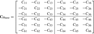
After some algebra, it can be shown that ZPhase is given by

where the elements of ZPhase are as given by Equation (3.75b).
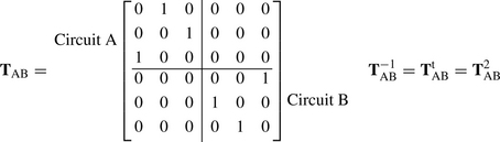
It is interesting to note the positions of the diagonal and off-diagonal elements of the inter-circuit mutual impedance matrix in comparison with those obtained in Equation (3.75a). The sequence impedance matrix of Equation (3.86) is calculated, noting the RYB/BYR phasing of circuits A and B, as follows:
where

and

Hdc is the transformation matrix for a double-circuit or two mutually coupled circuit line. The result takes the form of Equation (3.76a) with diagonal self-circuit and inter-circuit impedance matrices. The value of the sequence elements of the matrices are as given in Equation (3.76).
The above phase and sequence impedance matrix analysis for double-circuit lines applies equally to the line’s shunt phase and sequence susceptance matrices.
We have shown that with the use of six transpositions, the effect of mutual sequence coupling between the two circuits is not entirely eliminated with like sequence coupling between the two circuits remaining and this may indeed be the desired result. However, if required, it is even possible to eliminate the PPS and NPS coupling and retain ZPS coupling only between the two circuits. Because there are two three-phase circuits of conductors, each phase conductor has to be transposed within its circuit and with respect to the parallel circuit. In other words, if one circuit is subject to three transpositions, then for each one of its sections, the other circuit should undergo full three section transpositions. This produces a total of nine transpositions for our double-circuit line as shown in Figure 3.14.

Figure 3.14 Double-circuit line ideal nine transpositions with ZPS inter-circuit mutual coupling only
It can be shown analytically by inspection or by matrix analysis that the effect of this nine transposition assumption is to produce the following 6 × 6 phase impedance matrix:

where ZS(A), ZM(A), ZS(B) and ZM(B) are given in Equation (3.75b) and ZAB is given by
 (3.88b)
The elements of the inter-circuit mutual matrix are all equal to ZAB given in Equation (3.88b). This is equal to the average of all nine mutual impedances between the six conductors of the two circuits. The corresponding sequence matrix of Equation (3.88a) calculated using any electrical phasing of circuits A and B, e.g. RYB/RYB or RYB/BYR, is given by

 (3.89b)
Equation (3.88a) shows that the effect of this ultimate nine transposition assumption is to equalise all nine elements of the inter-circuit phase matrix. In the sequence reference frame, this eliminates the PPS and NPS mutual coupling between the two circuits but not the ZPS mutual coupling which will always be present. It is informative for the reader to derive the mutual phase impedance/susceptance matrices between the two circuits for all nine transpositions and show that the total has the form shown in Equation (3.88a).
3.2.7 Untransposed and transposed multiple-circuit lines
Multiple that is three or more three-phase circuits strung on the same tower or running in parallel in close proximity in a corridor are sometimes used in electrical power networks. Similar to double-circuit lines, mutual inductive and capacitive coupling exists between all conductors in such a complex multi-conductor system. Figure 3.15 illustrates typical three and four circuit tower arrangements. Two double-circuit lines may also run in close physical proximity to each other along the same route or right of way. The coupling between these lines is usually neglected in practice if the lines are electromagnetically coupled for a short distance only relative to the shortest circuit so that the effect on the overall electrical parameters of such a circuit is negligible. Where this is not the case the formulation of the phase impedance and susceptance matrices of the entire multi-conductor system and elimination of the earth wire(s) follows a similar approach to that presented in Section 3.2.5 for double-circuit lines. After the elimination of the earth wire(s), the dimension of the resultant phase matrix would be 3 × N where N is the number of coupled three-phase circuits. As in the case of double-circuit lines, the sequence impedance and susceptance matrices can be derived by introducing appropriate transposition assumptions to retain like sequence PPS, NPS and ZPS inter-circuit coupling but not intersequence coupling. Alternatively, ideal transpositions may be chosen so as to retain ZPS inter-circuit mutual coupling only.

Lines with three coupled circuits
Consider a line with three mutually coupled circuits 1, 2 and 3 erected on the same tower as illustrated in Figure 3.15(a). The transposed and balanced 9 × 9 series phase impedance matrix that retains PPS, NPS and ZPS inter-circuit mutual coupling can be derived using the technique presented for double-circuit lines. Each circuit is perfectly transposed within itself and the inter-circuit mutual impedance matrices between any two circuits result inequal self and equal mutual impedances. However, the inter-circuit mutual coupling impedances between circuits 1 and 2, circuits 1 and 3, and circuits 2 and 3 are assumed unequal to maintain generality. It can be shown that the resultant balanced phase impedance matrix is given by

The elements of this matrix can be calculated as for a double or two mutually coupled circuits given in Section 3.2.6 by averaging the appropriate self and mutual phase impedance terms of the original untransposed matrix.
For the ideal transposition the inter-circuit impedance matrices have all nine elements equal thereby retaining only ZPS inter-circuit mutual coupling. The ideal transposition assumption results in ZS12 = ZM12 = A12 for circuits 1 and 2, ZS13 = ZM13 = A13 for circuits 1 and 3, and ZS23 = ZM23 = A23 for circuits 2 and 3. The sequence impedance matrix can be calculated based on knowledge of the electrical phasings of the three circuits. The above series impedance matrix assumes that all circuits are phased RYB and the corresponding sequence impedance matrix can be calculated using
 (3.91)
giving

where
 (3.92b)
In the ideal transposition case where only ZPS inter-circuit mutual coupling is retained, we have ![]() .
.
The 9 × 9 transposed and balanced shunt phase susceptance matrix that retains PPS, NPS and ZPS inter-circuit mutual coupling, or ZPS inter-circuit mutual coupling only, is similar in form to the series phase impedance matrix. Similarly, the sequence susceptance matrix is similar in form to the sequence impedance matrix.
Lines with four coupled circuits
We now briefly outline for the most interested of readers the balanced phase impedance matrix for an unusual case of identical four circuits or two double-circuit lines running in close proximity to each other. In deriving such a matrix, it is assumed that each circuit is perfectly transposed and hence represented by a self and a mutual impedance. The inter-circuit mutual impedance matrices between any two circuits are also assumed balanced reflecting a transposition assumption similar to that for double-circuit lines. Further, the inter-circuit mutual coupling matrices between any two pair of circuits are assumed unequal to maintain generality. It can be shown that the balanced series phase impedance matrix of such a complex multi-conductor system with transpositions that retain PPS/NPS and ZPS inter-circuit mutual coupling is given by

Alternatively, an ideal transposition assumption results in C = D, E = F, G = H, J = K, L = M and U = W. The sequence impedance matrix that corresponds to Equation (3.93) can be calculated with all circuits phased RYB using
 (3.94)
where
 (3.95b)
In the ideal transposition case where only ZPS inter-circuit mutual coupling is retained, we have ![]() .
.
3.2.8 Examples
Example 3.1
Consider a single-circuit overhead line with solid non-magnetic conductors and no earth wire. Using the self and mutual impedance expressions for the phase conductors, and assuming the line is perfectly transposed, derive expressions for the PPS/NPS and ZPS impedances of the circuit. Ignore the conductor’s internal inductance skin effect.
Using Equation (3.19), the self and mutual impedances with earth return are given by
The nine elements of the original phase impedance matrix are calculated using Equation (3.50). Therefore, the PPS/NPS impedance is given by

where GMD = ![]() and GMR = 0.7788 × ro. It is interesting to note that the earth return resistance and reactance present in the self and mutual impedances with earth return cancel out and are not present in the PPS/NPS impedance. Using Equation (3.50), the ZPS impedance is given by
and GMR = 0.7788 × ro. It is interesting to note that the earth return resistance and reactance present in the self and mutual impedances with earth return cancel out and are not present in the PPS/NPS impedance. Using Equation (3.50), the ZPS impedance is given by

Example 3.2
Consider the double-circuit line shown in Figure 3.16 having a triangular conductor arrangement within each circuit and symmetrical arrangement with respect to the tower.

For the conductor numbering and electrical phasing given, prove that a three-cycle reverse transposition of circuit A and a similar but forward transposition of circuit B is sufficient to produce a balanced inter-circuit phase matrix and a diagonal inter-circuit sequence matrix.
From the geometry of the two circuits, the inter-circuit mutual impedance matrix of the three transposition sections can be written by inspection as follows:

Again, from the geometry of the circuits, we can write Z24 = Z15, Z26 = Z35, Z34 = Z16 and Z16 = Z34. Therefore, the inter-circuit phase impedance matrix is given by

and is balanced, and the corresponding diagonal sequence matrix is given by

Example 3.3
Consider a 275 kV single-circuit overhead line with a symmetrical horizontal phase conductor configuration and two earth wires. The spacing of the conductors relative to the centre of the tower and earth are shown in Figure 3.17. The crosses numbered 1–5 represent the mid span conductor positions due to conductor sag.

The physical data of conductors is as follows:
Phase conductors: 2 × 175 mm2 ACSR per phase, 30/7 strands (30 Aluminium, 7 Steel), conductor stranding factor = 0.82635, conductor outer radius = 9.765 mm, conductor ac resistance = 0.1586 ω/km, height at tower = 19.86 m, average sag = 10.74 m.
Earth wire conductor: 1 × 175 mm2 ACSR, 30/7 strands, outer radius = 9.765 mm, ac resistance = 0.1489 ω/km, height at tower = 25.9 m, average sag = 8.25 m.
Earth resistivity = 20 ωm Nominal frequency f = 50 Hz.
Calculate the potential coefficient and capacitance matrices, phase susceptance matrix with earth wires eliminated, perfectly transposed phase susceptance matrix and corresponding sequence susceptance matrix. Calculate the full phase impedance matrix, reduced phase impedance matrix with earth wires eliminated, perfectly transposed balanced phase impedance matrix, and sequence impedance matrices for the untransposed and balanced phase impedance matrices.
Average height of phase conductors = 19.86 – (2/3) × 10.74 = 12.7 m
Average height of earth wire conductor = 25.9 – (2/3) × 8.25 = 20.4 m
Potential coefficients, capacitance, phase and sequence susceptance matrices The GMR of each stranded conductor is equal to its radius i.e. GMRC = 9.765 mm. We have two subconductors per phase so GMREq = ![]() mm where the radius of a circle through the centres of the two conductors is equal to 300/2 = 150 mm.
mm where the radius of a circle through the centres of the two conductors is equal to 300/2 = 150 mm.


Therefore, the potential coefficient matrix is equal to

and the full phase capacitance matrix is equal to

Eliminating the two earth wires, the phase capacitance and susceptance matrices of the untransposed line are equal to

Assume phase conductors 1, 2 and 3 are phased R, Y and B, respectively,

Thus, the sequence susceptance matrix of the untransposed line is equal to

The self and mutual elements of the susceptance matrix of the perfectly transposed line are equal to
and
Thus, the balanced phase susceptance matrix is equal to

and the corresponding sequence susceptance matrix is equal to

Phase and Sequence impedance matrices
The GMR of each standed conductor is equal to GMRc = 0.82635 × 9.765 = 8.0693 mm. We have to subconductors per phase so GMREq = ![]() . The ac resistance per phase is equal to 0.1586/2 = 0.0793 ω/km. The depth of equivalent earth return conductor Derc = 658.87 ×
. The ac resistance per phase is equal to 0.1586/2 = 0.0793 ω/km. The depth of equivalent earth return conductor Derc = 658.87 × ![]() = 416.7 m. The phase impedances with earth return are equal to
= 416.7 m. The phase impedances with earth return are equal to
Therefore, the full phase impedance matrix is equal to

Eliminating the two earth wires, 4 and 5, the untransposed phase impedance matrix is calculated as follows

The corresponding sequence impedance matrix is equal to

The self and mutual elements of the impedance matrix of the perfectly transposed line are equal to

and

Thus balanced phase and corresponding sequence impedance matrices are

and

Example 3.4
Consider a 400 kV double-circuit overhead line with a near vertical phase conductor configuration and one earth wire. The conductors are numbered 1–7 and their spacings including average conductor sag relative to the centre of the tower and earth are shown in Figure 3.18.

The conductors of the two circuits have the following physical data.
Phase conductors: 4 × 400 mm2 ACSR per phase, 54/7 strands (54 Aluminium, 7 Steel), conductor stranding factor = 0.80987, conductor outer radius = 14.31 mm, conductor ac resistance = 0.0684 ω/km, Figure 3.18 shows average height of the centre of phase conductor bundle including average sag.
Earth wire conductor: 1 × 400 mm2 ACSR, 54/7 strands, outer radius = 9.765 mm, ac resistance = 0.0643 ω/km, Figure 3.18 shows average height of earth wire including average sag.
Earth resistivity = 20 ωm. Nominal frequency f = 50 Hz.
Calculate the 7 × 7 potential coefficient and capacitance matrices, 6 × 6 phase susceptance matrix with earth wire eliminated, the 6 × 6 phase susceptance matrix for six and ideal nine transpositions. Calculate the corresponding 6 × 6 sequence susceptance matrix in each case. Calculate the full 7 × 7 and reduced 6 × 6 phase impedance matrices with earth wire eliminated as well as the 6 × 6 phase matrices for six and ideal nine transpositions. Calculate the corresponding sequence impedance matrices in each case.
Potential coefficients, capacitance, phase and sequence susceptance matrices For each stranded conductor, the GMR is equal to GMRC = 14.31 mm. For the four conductor bundle, GMREq = ![]() = 224.267 mm
= 224.267 mm
where the radius of a circle through the centres of the four conductors is equal to R = 500 mm/![]() = 353.553 mm.
= 353.553 mm.

The rest of the self and mutual potential coefficients are calculated similarly. Therefore, the potential coefficient matrix is equal to

and the full-phase capacitance matrix is equal to C = P−1 or

Eliminating the earth wire, the phase capacitance and susceptance matrices of the untransposed line are equal to

The corresponding sequence susceptance matrix is calculated using BPNZ = ![]() BPhaseHdc. For the similar phasing of the two circuits, i.e. RYB/RYB, as illustrated in Figure 3.18, Hdc can be obtained by modifying Equation (3.87) appropriately giving
BPhaseHdc. For the similar phasing of the two circuits, i.e. RYB/RYB, as illustrated in Figure 3.18, Hdc can be obtained by modifying Equation (3.87) appropriately giving

For the circular phasing of the two circuits of RYB/BYR, as illustrated in Figure 3.18, Hdc is given in Equation (3.87). Therefore,

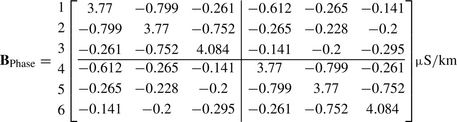
For the circular RYB/BYR phasing, and for a six-phase transposition cycle, the balanced phase susceptance and corresponding sequence susceptance matrices are equal to

and

For the ideal nine transpositions, the balanced phase susceptance and corresponding sequence susceptance matrices are equal to

and

Phase and sequence impedance matrices
The GMR of a stranded phase conductor is GMRC = 0.80987 × 14.31 = 11.589 mm. We have four subconductors per phase so GMREq = ![]() mm. The ac resistance per phase = 0.0684/4 = 0.0171 ω/km. The depth of equivalent earth return conductor Derc = 658.87 ×
mm. The ac resistance per phase = 0.0684/4 = 0.0171 ω/km. The depth of equivalent earth return conductor Derc = 658.87 × ![]() m.
m.
The GMR of the stranded earth wire is GMRC = 0.80987 × 9.765 = 7.91 mm. The phase impedances with earth return are equal to

The rest of the self and mutual phase impedances are calculated similarly. The full phase impedance matrix in Ω/km is equal to
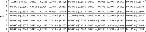
Eliminating the earth wire, the phase impedance matrix of the untransposed double-circuit-line is equal to

The corresponding sequence impedance matrix is ZPNZ = H![]() ZPhaseHdc. For similar phasing of the two circuits, i.e. RYB/RYB, as illustrated in Figure 3.18:
ZPhaseHdc. For similar phasing of the two circuits, i.e. RYB/RYB, as illustrated in Figure 3.18:
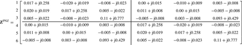
For the circular phasing of the two circuits of RYB/BYR, as illustrated in Figure 3.18, we obtain

For the RYB/BYR phasing, and for a six-phase transposition cycle, the balanced phase impedance and corresponding sequence impedance matrices are
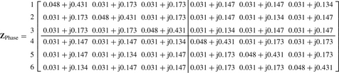

For the ideal nine transpositions, the balanced phase impedance and corresponding sequence impedance matrices are

The reader will benefit from carefully studying the results of the above examples which provide several insights of significant practical importance on natural overhead line unbalance and the effects of transpositions in the practice of electrical power systems engineering.
3.3 Phase and sequence modelling of three-phase cables
3.3.1 Background
Cables are generally classified as underground, submarine or aerial. Underground cables may be buried directly in the ground, laid in trenches, pipes or in underground tunnels. Cables are also classified depending on the type of core insulation, e.g. oil-impregnated paper, ethylene propylene rubber (EPR), or cross-linked polyethylene (XLPE), etc. Some cables may have a protective armour in addition to the metallic sheath or screen. Other classification is based on the number of cores, e.g. single core, two core or three core, etc. Single-core cables are coaxial cables with insulation that can either be extruded, e.g. XLPE or oil-impregnated paper. Self-contained fluid-filled cables consist of three single-core cables each having a hollow copper core which permits the flow of pressurised dielectric. High voltage cables are always designed with a metallic sheath conductor which may be copper, corrugated aluminium or lead. Three-core cables consist of three single-core cables contained within a common shell which may be an insulating shell or a steel pipe. There are a large number of different cable types, designs and layouts in use for the transmission and distribution of electrical energy and operating at voltages from 1 to 500 kV. It is therefore impossible to cover but a few cables focussing on those designs and layouts that are most commonly used. In some countries, e.g. the UK, distribution networks in large cities are almost entirely underground cable networks. Even at transmission voltage levels, increasing environmental and visual amenity pressures are resulting in more undergrounding of cables in addition to some of the usual requirements imposed by wide rivers and sea crossings. At the lower end of distribution voltages, belted-type cables have been used and these are three-core cables usually insulated with solid oil-impregnated paper with the three conductors covered in a single metallic sheath. At operating voltages between 10 and 36 kV, three-core cables are becoming mainly of the screened type with polymeric insulation and outer sheath applied to each core. Above 36 kV, cables have historically been fluid-filled paper-insulated but more recently, the use of such cables has mainly been above 132 kV. In the last few years, XLPE-insulated cables are increasingly being used at voltages up to 500 kV. Cables used at transmission voltages are mostly single-core cables that may be laid in a variety of configurations in the ground, tunnels or pipes.
The ac submarine cables are similar to underground cables except that they invariably have a steel armour for mechanical protection and this consists of a number of steel wires or tapes. Submarine cables may be three-core cables buried underneath the seabed at between 1 to 2 m depth to avoid damage by ships’ anchors, fishing trawlers or possibly physical displacement in areas of high sea currents. Submarine cables may also be single core and buried under the seabed but where this is not the case, e.g. in deep water installations, the individual phases may be laid a significant distance away from each other to minimise the risk of anchors damaging more than one phase. Pipe-type cables consist of three single-core cables each usually having a stranded copper conductor, impregnated paper insulation and a metallic sheath. The three cables may be installed asymmetrically or in a trefoil formation inside a steel pipe which is filled with pressurised low-viscosity oil or gas. The three sheaths are in contact with the pipe inside wall and they may touch each other. The steel pipe is normally coated on the outside to prevent corrosion. In the USA, over 90% of underground cables from 69 kV up to 345 kV are of pipe-type design but many modern replacement and new installations are employing oil-free XLPE cables with forced water cooling inside the pipe. In England and Wales, almost all transmission cables are of the self-contained single-core design laid either directly in trenches underground or in tunnels. At the time of writing, single-core XLPE cables up to 500 kV and three-core XLPE cables up to 245 kV are in use.
3.3.2 Cable sheath bonding and earthing arrangements
Cable sheaths are metallic conductors that perform a variety of important functions. The sheaths prevent moisture ingress into the insulation, contain cable pressure in fluid-filled cables, provide a continuous circuit for short-circuit fault current return and help prevent mechanical damage. Three cables form a three-phase single circuit and two such three-phase circuits may be laid in close proximity to each other. The ac current flowing in the core of one cable, as well as the currents flowing in adjacent cores, induce voltages on the metallic sheath(s) of the cable(s). In order to limit these voltages and prevent cable damage, the conducting sheaths may be bonded in a variety of methods. The three most common methods are briefly described below.
Solidly bonded cables
Solid bonding of cable sheaths is where both ends of the cable are bonded and connected to earth as shown in Figure 3.19.

Under PPS voltage conditions, voltages are induced in the sheaths and because these are solidly bonded and earthed at both ends, circulating currents flow such that the sheaths are at zero voltage along their entire length. However, these currents can cause significant sheath losses and heating which can adversely affect the thermal rating of the cable’s core conductor. This arrangement is most suitable for three-core cables and is not usually used at voltages above 66 kV. Under ZPS conditions, the sheaths provide an excellent path for the earth fault return current.
Single-point bonded cables
Bonding the cable sheaths to earth at one end and using sheath voltage limiters at the other end is a good arrangement for short cable lengths. This limits the sheath voltages and prevents circulation of sheath currents during normal operation because of the absence of a closed sheath circuit. A similar arrangement that provides similar benefits and allows doubling the cable length is bonding and earthing the cable sheath at the cable mid-point and using sheath voltage limiters at the ends. Because no sheath current can flow, no sheath losses occur. However, in practical installations, a transposed earth continuity conductor earthed at both ends is also used in order to provide a return path for the current under ZPS earth fault conditions. Under PPS conditions, the transposed earth continuity conductor carries no current. Figure 3.20 illustrates these three earthing arrangements.

Cross-bonded cables
For long cable circuits, cross-bonding is commonly used. This method aims at minimising the total induced voltages in the sheath in order to minimise circulating currents and losses. The cable circuit is divided into major and minor sections so that each major section consists of three minor sections of equal length. Figure 3.21 illustrates a major section of a cross-bonded cable.
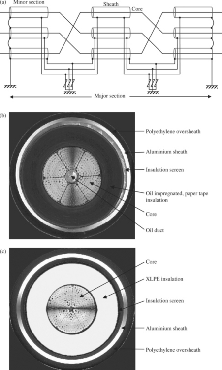
Figure 3.21 (a) Cross-bonded three-phase cable; (b) 275 kV oil-filled paper insulated cable and (c) 400 kV cross-linked polyethylene (XLPE) cable
The best arrangement is where the cores of the three minor sections within each major section are perfectly transposed but the sheaths are not. The sheaths at both ends of the major section are solidly bonded and earthed but at the other two positions within the major section, they are bonded to sheath voltage limiters. The bonding and earthing at the ends of a major section eliminate the need for the earth continuity conductor required in single-point bonded and earthed arrangements.
Under PPS conditions, voltages are induced in the sheaths, but because the cores are perfectly transposed, the resulting voltages in each minor section are separated by 120° and thus sum to zero. Therefore, no sheath currents flow. Under ZPS conditions, e.g. earthed faults, the cross-bonding does not affect the excellent path which the sheaths provide for the return current. The earlier and rather less satisfactory cross-bonding method of transposing the sheaths but not the cores cannot achieve a good balance of induced sheath voltages unless the cables are laid in a trefoil formation. Therefore, the cores of cross-bonded cables laid in flat formations are generally transposed. Cross-bonding with core transposition is a general practice in the UK at 275 and 400 kV.
3.3.3 Overview of the calculation of cable parameters
General
Single-core and three-core cables are characterised by close coupling between the core conductor and the conducting sheath. Also, for buried self-contained single-core cables, there is a conducting earth path between the three adjacent conductors. In pipe-type cables, the steel pipe is also a conducting medium. Therefore, a single circuit self-contained three-phase cable is a multi-conductor system that consists of three cores and three sheaths (six conductors) together with the earth path. If the three cables are in a steel pipe, induced voltages in the pipe will cause currents to circulate. For single-core submarine cables where each has a conducting armour, a three further conductors are present. Therefore, for N three-phase cable circuits, the number of coupled conductors is 6N for core–sheath single–core or three–core cables, and 9N for core–sheath–armour single-core cables. For core–sheath–armour single-circuit three-core cables, the total number of coupled conductors is seven.
Similar to an overhead line, the basic electrical parameters of cables are the self and mutual impedances between conductors, and conductor shunt admittances. For power frequency steady state analysis, the small conductance of the insulation is usually neglected. Practical calculations of multi-conductor cable parameters with series impedance expressed in ω per-unit length and shunt susceptance in μ S unit length, are carried out using digital computer programs. These parameters are then used to form the cable series impedance and shunt admittance matrices in the phase frame of reference as will be described later. The cable capacitances or susceptances are calculated from the cable physical dimensions and geometry. The self and mutual impedances are calculated from the conductor material, construction, physical dimensions and earth resistivity. The significant variety of available cable designs and installations cannot be covered here. The equations of the parameters for some widely used cable designs are presented below.
Shunt capacitances and susceptances
For single-core screened cables where the phases are laid parallel to each other and to the earth’s surface, the earth the screens are connected to acts as an electrostatic shield so that there is no electrostatic coupling between the phases. This also applies to three-phase three-core screened cables where each core is individually screened. Therefore, there is no mutual capacitance among the three phases and the individual cable capacitance is independent of the spacings between the phases. Figure 3.22 is a cross-section of a general cable showing a hollow core conductor, core insulation, sheath/screen conductor, sheath insulation, armour conductor and a further insulation layer such as a plastic sheath.

Using Figure 3.22, the capacitance between the core and sheath of a screened single core or a screened three-core cable is given by
 (3.96a)
and the corresponding susceptance is given by
 (3.96b)
The capacitance between the sheath and armour, where present, is given by
 (3.97a)
and the corresponding susceptance is given by
 (3.97b)
Similarly, the capacitance between the armour and earth is given by
 (3.98a)
and the corresponding susceptance is given by
 (3.98b)
where
ric = inner radius of core tubular conductor
roc = outer radius of core conductor = inner radius of core conductor insulation assuming no core semiconductor tape
ris = outer radius of core conductor insulation = inner radius of metallic sheath assuming no tape over insulation
ros = outer radius of metallic sheath = inner radius of sheath insulation
ria = inner radius of metallic armour = outer radius of sheath insulation
roa = outer radius of metallic armour = inner radius of metallic armour’s plastic sheath
tps = thickness of metallic armour’s plastic sheath
εcs, εsa and εae are the relative permittivities of core-to-sheath, sheath-to-armour and armour-to-earth insulation.
The capacitance between the armour and earth would be redundant if there were no armour insulation or where the armour is directly earthed. Similarly, this capacitance would not exist for cables that have no armour and in this case, the cable would generally be characterised by two capacitances only. The relative permittivity of insulation is in general a complex number with frequency dependent real and imaginary parts, i.e. εr = ε′(f) –jε″(f). However, for power frequency steady state analysis, only the real part of εr is of significance and this is equivalent to assuming zero shunt conductance. Typical values for the real part of εr are: 4 for solid-impregnated paper, 3.5 for oil-filled-impregnated paper, 3.7 for oil-pressure pipe-type, 3.5 for gas-pressure, 4 for butyl rubber (BR), 3 for EPR, 2.5 for XLPE, 2.3 for polyethylene (PE) and 8 for polyvinyl chloride (PVC).
For three-phase pipe-type cables, the cables inside the pipe may be laid in a touching triangular or a cradle formation as illustrated in Figure 3.23. The core-to-sheath capacitance of each cable phase can be calculated using Equation (3.96a).
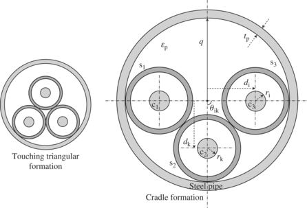
Mutual capacitances between the sheaths of the three phases and between the sheath of each phase and the pipe can be calculated using
 (3.99a)
and
 (3.99b)
where q is the inner radius of the steel pipe, εp is the permittivity of insulation inside the pipe, di is the distance between cable i core centre and pipe centre, ri is the outer radius of cable i core conductor and θik is the angle subtended between the pipe’s centre and the centres of cables i and k. The infinite series term in Equation (3.99a) is usually very small and for most di and q distances encountered in practical installations, it may be neglected with insignificant loss of accuracy. It should be noted that the mutual sheath capacitance would be short-circuited where the sheaths are in contact with each other, and the pipe’s inside wall. This applies for both cradle and triangular formations.
For three-core unscreened or belted cables, there is no simple reasonably accurate formula that can be used because of the effect of two insulation layers that have to be considered namely the core insulation and the belt insulation. For these cables, it is recommended that resort is made either to empirical design data from the manufacturers or better still to field test measurements. This is dealt with in Section 3.6.3.
Series self and mutual impedances
For a three-phase screened cable buried underground and having armour protection, the core, sheath and armour will each have a self-impedance with earth return. Electromagnetic coupling, and hence mutual impedances, exist between the core, sheath and armour within each phase. Even though the three phases are usually laid parallel to each other and the earth’s surface, the earth does not act as an electromagnetic shield between them. Therefore, mutual impedances exist between all the conductors of all the phases. Figures 3.22 and 3.24 are used in the calculation of self and mutual impedances of underground cables for use in steady state power frequency analysis.

The self-impedance of a core conductor with earth return is given by
where
 (3.100b)
and Derc is the depth of equivalent earth return conductor given in Equation (3.15) and μc is the relative permeability of the core conductor.
The self-impedance of a sheath with earth return is given by
 (3.101b)
and μs is the relative permeability of the sheath conductor.
The self-impedance of an armour with earth return is
where
 (3.102b)
and μa is the relative permeability of the armour conductor.
The mutual impedance between core or sheath or armour i, and core or sheath or armour j, with earth return, is given by
where Sij is the distance between the centres of cables i and j if the conductors belong to different cables. If the conductors belong to the same cable, Sij is the geometric mean distance between the two conductors, e.g. the GMD between the core and the sheath of cable j is given by Sjj = (ros + ris)/2 which is sufficiently accurate for practical cable dimensions.
ac resistance
The ac resistance of the core, sheath or armour can be calculated from the dc resistance using the following formula:
where y = 1 for single-core, two-core and three-core cables but y = 1.5 for pipe-type cables. kS and kP are skin and proximity effect factors, respectively. Also,
ρ is the conductor resistivity in ωm, A is conductor nominal cross-sectional area in m2, T is conductor temperature in °C and α20 in °C−1 is the constant mass temperature coefficient at 20°C. Table 3.1 illustrates typical values for α20 and resistivity at 20°C.
Table 3.1 Typical values of α20 and conductor resistivity at 20°C
| Material | Temperature coefficient α20(°C−1) at 20°C | Resistivity ρ20 (Ωm) at 20 °C |
|---|---|---|
| Cores | ||
| Copper | 3.93 × 10⁻³ | 1.7241 × 10⁻⁸ |
| Aluminium | 4.03 × 10⁻³ | 2.8264 × 10⁻⁸ |
| Sheaths or armour | ||
| Lead | 4 × 10⁻³ | 21.4 × 10⁻⁸ |
| Bronze | 3 × 10⁻³ | 3.5 × 10⁻⁸ |
| Steel | 4.5 × 10⁻³ | 13.8 × 10⁻⁸ |
| Stainless steel | 0 | 70 × 10−8 |
The skin effect factor is the incremental resistance factor produced by ac current in an isolated conductor due to skin effect and is given by
 (3.105)
where z = ![]() . For copper conductors, az = 1 for normally stranded circular and sector-shaped conductors but az = 0.43 for segmental or Milliken shaped conductors. For stranded annular conductors, az = [(ro – ri)/(ro + ri)][(ro + 2ri)/(ro + ri)]2, where ri and ro are the conductor’s inner and outer radii, respectively. Generally, z is less than 2.8 for the majority of practical applications. Although based on a simplified approach, Equation (3.105) for the skin effect factor involves an error of less than 0.5% at power frequency.
. For copper conductors, az = 1 for normally stranded circular and sector-shaped conductors but az = 0.43 for segmental or Milliken shaped conductors. For stranded annular conductors, az = [(ro – ri)/(ro + ri)][(ro + 2ri)/(ro + ri)]2, where ri and ro are the conductor’s inner and outer radii, respectively. Generally, z is less than 2.8 for the majority of practical applications. Although based on a simplified approach, Equation (3.105) for the skin effect factor involves an error of less than 0.5% at power frequency.
The proximity effect factor is the incremental resistance factor due to the proximity of other ac current carrying conductors and is given by
 (3.106a)
where
 (3.106b)
dc is conductor diameter and S is the axial spacing between conductors. For both copper and Aluminium, ap is equal to 0.8 for round stranded, sector shaped and annular stranded conductors. ap is equal to 0.37 for round segmental conductors.
The values of the various factors used in Equations (3.104), (3.105) and (3.106) are usually supplied by the cable manufacturer.
For a three-phase submarine cable, the power frequency equations given for underground cables can be used. However, the sea will now predominantly replace earth as the return path and is represented as follows:
where Rsea is the outer radius of sea return represented as an equivalent conductor and ρSea is the resistivity of sea water. This concept is derived from the calculation of sea return impedance where the cable is assumed to be completely surrounded by an indefinite sea that acts as an equivalent return conductor having an outer radius of RSea. For example, for a typical value of sea water resistivity of ρSea = 0.5 ωm, RSea ≅ 40 m at 50 Hz. It is interesting to note that in deep sea water, where the cable phases are laid 100 to 500 m apart, electromagnetic coupling between the phases would be very weak and can be normally ignored. The internal impedance of the sea return represented as an equivalent conductor of radius RSea is given by
where α = 1.123 × D/RSea, D is mean spacing between the cable’s phases in m, r is conductor radius in m, and ker(α) and kei(α) are Kelvin functions with a real argument α.
For pipe-type cables, the calculation of the self and mutual impedances is more complex than for buried underground cables. The calculation of the flux linkages within the wall of the steel pipe and outside the pipe is further complicated by the non-linear permeability of the steel pipe which itself varies with the magnitude of ZPS current flowing through the pipe under earth fault conditions due to pipe saturation. The effect of saturation is to cause a reduction in the effective ZPS impedance of the cable; the larger the ZPS current, the larger the reduction in ZPS impedance. Cable manufacturers are usually required to provide such data to network utilities. For power frequency analysis, a usual assumption is that the pipe’s thickness is greater than the depth of penetration into the pipe wall and that this assumption remains approximately true under increased pipe ZPS current. This means that besides the sheaths of the three cables, the pipe is the only current return path and that no current returns through the earth. The cables inside the pipe can then be considered as three self-contained single-core cables but with the pipe replacing the earth as the current return path. The depth of penetration into the pipe can be calculated using the skin depth formula of Equation (3.7b) ![]() where ρp and μp are the pipe’s resistivity and relative permeability respectively. To illustrate the assumption of infinite pipe thickness, consider a steel pipe of a 132 kV pipe-type cable having a thickness of 6.3 mm, a resistivity of ρp = 3.8 × 10⁻⁸ ωm and a relative permeability μp = 400. The depth of penetration into the pipe at 50 Hz is equal to δ = 1.32 mm. This is smaller than the pipe’s thickness and illustrates that the return current will flow towards the inner wall of the pipe and that the earth return can be ignored. In Figure 3.23, we assume that each cable phase consists of a solid core conductor of radius rc, core insulation and a sheath conductor of inner and outer radii ris and ros, respectively. From Figure 3.23, the self-impedance matrix of cable phase k inside the pipe is given by
where ρp and μp are the pipe’s resistivity and relative permeability respectively. To illustrate the assumption of infinite pipe thickness, consider a steel pipe of a 132 kV pipe-type cable having a thickness of 6.3 mm, a resistivity of ρp = 3.8 × 10⁻⁸ ωm and a relative permeability μp = 400. The depth of penetration into the pipe at 50 Hz is equal to δ = 1.32 mm. This is smaller than the pipe’s thickness and illustrates that the return current will flow towards the inner wall of the pipe and that the earth return can be ignored. In Figure 3.23, we assume that each cable phase consists of a solid core conductor of radius rc, core insulation and a sheath conductor of inner and outer radii ris and ros, respectively. From Figure 3.23, the self-impedance matrix of cable phase k inside the pipe is given by
 (3.109)
where Z1 is as given in Equation (3.7), and
 (3.110a)
 (3.110b)
 (3.110c)
where Z1 to Z6 are in ω/km. Ii and Ki are modified Bessel functions of the first and second kind of order i, respectively. The pipe’s internal impedance with the return path being the inside wall of the pipe is given by
 (3.111)
The mutual impedance in ω/km between the ith and kth conductor with respect to the pipe’s inner wall is given by
 (3.112)
where K′n is the derivative of Kn.
3.3.4 Series phase and sequence impedance matrices of single-circuit cables
General
Having calculated the basic phase parameters in Section 3.3.3, we will now derive the cable’s phase and sequence impedance matrices. We use the suffixes C, S and A to denote core, sheath and armour conductors respectively for cable phases 1, 2 and 3. Figure 3.25 shows six practical cable layouts for three-core and single-core cables. Pipe-type cables were shown in Figure 3.23.

Cables with no armour
A three-phase single-core or shielded three-core cable has a total of six conductors; three cores and three sheaths as shown in Figure 3.26a.

Figure 3.26 Multi-conductor cables with sheaths and armours: (a) cable conductors, no armour and (b) cable conductors, with armour
The series voltage drop per-unit length across the cores and sheaths is calculated from the cable’s full impedance matrix, core and sheath conductor currents and is given by

where ZCC and ZSS are the core and sheath self-impedances with earth return, respectively, and ZCS is the mutual impedance between core and sheath with earth
return. Equation (3.113) can be simplified depending on the cable layout and spacings between the phases as shown in Figure 3.25.
Three-core cables, three single-core cables in touching trefoil layout and three-single-core cables in equilateral layout
These three cable layouts, shown in Figure 3.25 are fully symmetrical. From the configuration of these cables, a number of practical equalities can be deduced as follows:
 (3.114)
Therefore, the cable full impedance matrix of Equation (3.113) can be written as
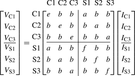
or
 (3.115b)
where
 (3.115c)
It is interesting to observe that the matrices ZCC, ZCS and ZSS are all balanced matrices since all diagonal terms are equal and all off-diagonal terms are equal. This is due to the symmetrical cable layouts. Where the cable sheaths are solidly bonded and earthed at both ends, the sheaths can be eliminated. Therefore, the phase impedance matrix involving the cores only can be calculated by setting VS = 0 in Equation (3.115b). The resultant core or phase impedance matrix is given by
 (3.116)
Because the individual impedance matrices ZCC, ZCS and ZSS are all balanced, the resultant phase impedance matrix ZPhase, that includes the effect of the eliminated sheaths, will also be balanced. The reader is encouraged to prove this statement. Therefore, the sequence impedance matrix is given by ZPNZ = H−1ZPhaseH or
 (3.117a)
where
Single-core cables in a trefoil layout
Using Figure 3.25 and following similar steps, it can be shown that the cable full impedance matrix of Equation (3.113) can be written as

where
 (3.118b)
The calculation of the phase impedance matrix involving the cores only and the corresponding sequence impedance matrix follows the same steps as above. However, in this case, the phase impedance matrix will not be balanced and as a result, the sequence impedance matrix will contain off-diagonal intersequence mutual terms.
Single-core cables in a flat layout
The general asymmetrical flat layout of single-core three-phase cables is shown in Figure 3.25. From the configuration of the cable, we can write the following equalities
 (3.119)
Therefore, the cable full impedance matrix of Equation (3.113) can be written as

For cross-bonded cables shown in Figure 3.21, the cores of the minor sections are transposed so that each occupies the three positions, but the sheaths are not. This is illustrated in Figure 3.27.
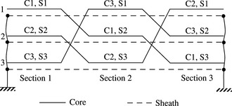
Equation (3.120a) is the full impedance matrix of the first minor section. The full impedance matrices of the second and third minor sections are given by

Using Equation (3.120) and all impedances are in per unit length i.e. ω/km, the full impedance matrix of a cross-bonded cable with transposed cores in each major section is given by

or

or including core and sheath voltage vectors
 (3.121b)
As expected, the core matrix ZCC is balanced, due to the perfect core transpositions assumed but the sheath matrix ZSS is not because the sheaths are untransposed. The mutual impedance matrix between the cores and the sheaths ZCS is also unbalanced.
In both cases of a solidly bonded cable where the sheaths are bonded and earthed at the cable ends, and the case of a cross-bonded cable where the sheaths are bonded and earthed at the ends of major sections, the phase impedance matrix involving the cores only can be calculated by setting VS = 0 in Equation (3.121b). Therefore, the core or phase impedance matrix takes the following general form
 (3.122)
The elements of the matrix ZPhase are the self-impedances of each phase (core) and the mutual impedances between phases (cores) with the sheaths and earth return included. Generally, for solidly bonded cables, the self or diagonal terms of ZPhase are not equal among each other nor are the off-diagonal mutual terms. In other words, the matrix is generally not balanced. This might also be expected to be the case for cross-bonded cables but in practical cable spacings and layouts, the core transposition eliminates the unbalance. The general sequence impedance matrix equation that corresponds to Equation (3.122), calculated using ZPNZ = H−1ZPhaseH, is given by
 (3.123)
where ZPP, ZNN and ZZZ are the PPS, NPS and ZPS impedances of the cable and ZPP = ZNN. The off-diagonal terms are intersequence mutual terms which are normally small in comparison with the diagonal terms for solidly bonded cables and practically negligible for cross-bonded cables.
For a cable that is solidly bonded and earthed at its centre and a transposed earth continuity conductor is used, two full impedance matrices would need to be built for each half of the cable including the earth continuity conductor then combined into a single matrix. The calculation of the phase impedance matrix of such a cable makes use of the fact that no current can flow in the sheath that is IS = 0. The derivation of the phase impedance matrix for such a cable is left for the reader.
Cables with armour
Some land based cables and almost all submarine cables have metallic armour. The armour acts as a third conductor in addition to the core and the sheath.
Single-core armoured cables
Using Figure 3.26(b)(i) for single-core armoured cables, the series voltage drop per-unit length is given by

In order to control the voltages between the sheath and the armour, the sheath is usually bonded to the armour at a number of points along the route. The armour covering is not normally an electric insulation so that the armour, and the sheath bonded to it, are effectively earthed. Therefore, the calculation of the cable’s phase (core) impedance matrix requires the elimination of both sheath and armour. Writing Equation (3.124) in partitioned matrix form, we have

The sheaths and armours are eliminated by setting VS = VA = 0 in Equation (3.125) and combining their matrices as follows:
Therefore, the phase (core) impedance matrix of the cable with sheaths, armours and earth, or sea water in the case of a submarine cable, constituting the current return path, is obtained as follows:
For single-core submarine cables where the individual phases are laid physically far apart from each other, the mutual electromagnetic coupling between the phases may be so weak that it can be neglected. Therefore, from the configuration of such three-phase submarine cables, a number of practical equalities can be deduced as follows:
 (3.127)
and all mutual terms between the three phases of the cables are zero. Therefore, Equation (3.124) simplifies to

Using Equation (3.126b), the phase (cores) impedance matrix is given by
 (3.129a)
where Zα = d – (a2f + b2e − 2abc) or using Equation (3.127),
Zα is the impedance of each core or phase including the effect of the combined sheath, armour and sea water return. The corresponding PPS/NPS and ZPS sequence impedances for the cable are all equal to Zα which is a direct result of the absence of mutual coupling between the three phases.
In the case where the distances between the phases are not so large that the mutual coupling between them cannot be ignored, three further impedance parameters need to be defined to account for the interphase coupling. Let the mutual impedance parameter between phases 1 and 2 be g such that
The mutual impedances between phases 1 and 3, and phase 2 and 3 are similarly defined. The analysis for calculating the cable phase impedance matrix proceeds as above.
Three-core armoured cables
Using Figure 3.26(ii) for three-core armoured cables, there are three cores and three sheaths but only one armour. Thus, the series voltage drop per-unit length is given by

Using the equalities of Equation (3.114) for the case with no armour, and the new equalities
we can write

As for the single-core cable, where the sheaths and armours are bonded and earthed, we can now eliminate the sheaths and armour by combining the matrices that correspond to them by setting VS = VA = 0. Writing Equation (3.131) in partitioned form, we have
 (3.132a)
The phase (core) impedance matrix of the cable with sheath, armour and earth, or sea water in the case of a submarine cable, constituting the current return path, is given by
The phase (core) impedance matrix will virtually be balanced. The corresponding sequence impedance matrix calculated using ZPNZ = H−1ZPhaseH will be a diagonal matrix, i.e. having virtually no intersequence terms. The diagonal terms are the required PPS/NPS and ZPS impedances.
Pipe-type cables
Using Figure 3.23 for a three-phase pipe-type cable, there are three cores, three sheaths and one pipe which represents the return path, i.e. a total of seven conductors. Therefore, the full cable impedance matrix takes the form of Equation (3.130) with armour ‘A’ replaced with pipe ‘P’. The elimination of the pipe only or pipe and sheaths can be carried out as described above.
3.3.5 Shunt phase and sequence susceptance matrices of single-circuit cables
In this section, we derive the cable phase and sequence susceptance matrices using the basic phase parameters calculated in Section 3.3.3.
Screened cables with no armour
For screened three-core and screened single-core cables, we have already established that there is no capacitance between one cable phase and another. From Figure 3.22, we note that there are two capacitances, or susceptances, corresponding to the core insulation and the sheath insulation layers and these are illustrated in Figure 3.28(a).

For each phase, the core and sheath current/voltage equations can be written as IC = jBCS(VC – VS) and IC + IS = jBSEVS where BCS and BSE are the core-to-sheath and sheath-to-earth susceptances, respectively. Therefore, writing similar equations for the three cores and three sheaths, the full shunt susceptance matrix is given by

For solidly bonded and cross-bonded cables, the sheaths can be eliminated using VS1 = VS2 = VS3 = 0. The resultant shunt phase (cores) susceptance matrix is given by
 (3.134)
that is the PPS, NPS and ZPS susceptances are all equal, and equal to BCS.
For cables that are bonded and earthed at one end only or at the cable centre, there will also be a capacitance or susceptance between the earth continuity conductor and earth with IECC = jBECC-EVECC. This increases the dimension of the full admittance matrix given in Equation (3.133) by one row and one column, i.e. from 6 × 6 to 7 × 7. The calculation of the 3 × 3 phase susceptance matrix for such cables, the constraint that no sheath current can flow, i.e. IS1 = IS2 = IS3 = 0 is applied. The resultant phase (cores) susceptance matrix is given by
 (3.135a)
This result shows that the cable-to-sheath capacitance and the sheath-to-earth capacitance of each core are effectively in series as can be seen from Figure 3.28(a).
The corresponding shunt sequence susceptance matrix of Equations (3.134) and (3.135a) is given by
that is the PPS, NPS and ZPS susceptances are all equal to the relevant phase susceptances.
Screened cables with armour
From Figure 3.22, we note that there are three capacitances, or susceptances, corresponding to the core insulation layer, the sheath insulation layer and the armour coating where this is made of insulation material. These are illustrated in Figure 3.28(b). For each phase, the core, sheath and armour current/voltage equations can be written as
and
Therefore, writing similar equations for the three cores, three sheaths and three armours, the full shunt susceptance matrix B is given by

If the sheath and armour are bonded together and earthed at both ends, then circulating currents can flow through the sheath and armour in parallel with earth return, or sea water return in the case of a submarine cable. The phase (core) susceptance matrix is easily obtained by deleting the last six rows and columns that correspond to the sheath and armours. The earthing of the sheath and armour, in effect, short circuits the sheath-to-armour and armour-to-earth capacitances as can be seen in Figure 3.28(b). The PPS, NPS and ZPS susceptances in equal to the phase susceptance BCS. If the sheath and armour are unearthed or earthed at one point only, then no sheath or armour current would flow and the equivalent core or phase capacitance is equal to the three capacitances of Figure 3.28(b) in series that is
Unscreened or belted cables
Belted cables are three-core cables where each core has an insulation layer but no screen or metallic sheath. There is also a belt insulation layer around all three cores and a single metallic sheath cover as illustrated in Figure 3.29(a).
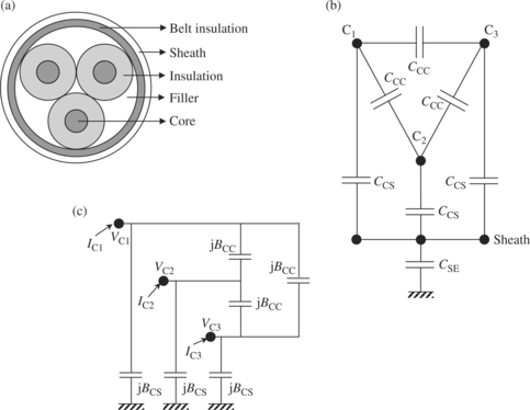
Figure 3.29 Three-core belted cable and capacitance equivalent circuits: (a) cross-section of a three-phase belted cable; (b) capacitance equivalent circuit and (c) capacitance equivalent circuit with earthed sheath
There are capacitances among the three cores, between each core and sheath and between the sheath and earth. Figure 3.29(b) shows the equivalent capacitance circuit of the cable where CCC is the core-to-core capacitance, CCS is the core-to-sheath capacitance and CSE is the sheath-to-earth capacitance. Where the sheath is solidly earthed, as is usually the case, the equivalent capacitance circuit reduces to that shown in Figure 3.29(c). The injected currents into the three cores can be expressed as follows:
and similarly for the two remaining cores. The nodal phase susceptance matrix is
 (3.138a)
and the corresponding sequence susceptance matrix is given by
 (3.138b)
where
It is interesting to note that the ZPS susceptance of a belted cable is smaller than its PPS/NPS susceptance. This contrasts with the equal PPS/NPS and ZPS susceptances of screened three-core and single-core cables. It is useful to calculate the core-to-core cable susceptance in terms of the sequence susceptances giving BCC = (BP – BZ)/3.
3.3.6 Three-phase double-circuit cables
In some installations, double-circuit cables may be laid close to each other. These may be three-core circuits or single-core circuits laid in flat or trefoil arrangements. Near vertical arrangements may be used in tunnels. We will describe the case of single-core unarmoured cables. As each circuit consists of six conductors, three cores and three sheaths, twelve conductors form this complex mutually coupled multi-conductor arrangement. Let the two circuits be designated A and B and let C1, C2, C3, S1, S2 and S3 be the cores and sheaths of circuit A, C4, C5, C6, S4, S5 and S6 be the cores and sheaths of circuit B. The full 12 × 12 impedance matrix is given by

or in concise matrix form, including voltage drop and current vectors

In practical installations, various double-circuit cable earthing arrangements may be used. Some of these are: circuit A and circuit B are solidly bonded, circuit A and circuit B are cross-bonded, circuit A and circuit B are single-point bonded, circuit A is solidly bonded in a trefoil formation and circuit B is single-point bonded in a flat formation, etc. The matrix of Equation (3.139) can be modified for any of these arrangements to calculate the reduced 6 × 6 phase impedance matrix for the two circuits that include their cores only. Figure 3.30 shows one arrangement where circuit A and circuit B are both cross-bonded with identical core transposition arrangements.
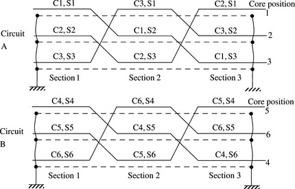
It is instructive for the reader to use the methodology presented in the single-circuit case to calculate the average 12 × 12 impedance matrix for the transposed double-circuit cable from the 12 × 12 matrix of each minor section. Using Equation (3.139b), this average 12 × 12 matrix can be written as follows:
 (3.140a)
The calculation of the 6 × 6 phase impedance matrix of the cores only, with both circuits loaded, makes use of VS(A) = VS(B) = 0 or VS(AB) = 0 in Equation (3.140a) giving
where
Equation (3.140b) can be rewritten as follows:
 (3.141a)
If one circuit, e.g. circuit A, is open-circuited, i.e. the cores carry no currents, IC(A) = 0 and the resultant 3 × 3 matrix for circuit B is directly obtained as ZPhase(B)3 × 3. If circuit A is open and earthed, then the resultant 3 × 3 impedance matrix of circuit B is derived using VC(A) = 0 in Equation (3.141a) giving
These are practical cases that can arise in normal power system design and operation for which the cable impedance parameters would be required.
3.3.7 Examples
Example 3.5
A 275 kV underground self-contained three-phase cable laid out in a symmetrical flat arrangement as shown in Figure 3.31.

The cable’s geometrical and physical data are as follows:
Copper core: inner radius = oil duct radius = 6.8 mm, outer radius = 21.9 mm, relative permeability = 1.0, ac resistance = 0.01665 ω/km.
Core insulation: paper, relative permeability = 1.0, relative permittivity = 3.8.
Lead sheath: inner radius = 37.9 mm, outer radius = 40.9 mm, relative permeability = 1.0, ac resistance = 0.28865 ω/km.
PVC over-sheath: thickness = 3 mm, relative permittivity = 3.5, relative permeability = 1.0.
Earth resistivity = 20 ωm. Nominal frequency f = 50 Hz.
Calculate the phase and sequence susceptance and impedance parameters for a solidly bonded cable and a cross-bonded cable whose cores are perfectly transposed in each major section.
The core insulation susceptance is equal to
and the PVC over-sheath susceptance is
The full susceptance matrix of the cable is equal to

The phase and sequence susceptance matrix for a solidly bonded or cross-bonded cable is given by

Depth of earth return conductor ![]() m. For the tubular core conductor
m. For the tubular core conductor

thus


All mutual impedances between cable phase 1 core and sheath conductors, and cable phase 2 core and sheath conductors are equal, and similarly for those impedances between cable phases 2 and 3. The full impedance matrix is equal to

For a solidly bonded cable, the phase impedance matrix is equal to

and the corresponding sequence impedance matrix is equal to
ZP = ZN = (0.043 + j0.129)ω/km and ZZ = (0.292 + j0.1)ω/km.
For a cross-bonded cable, the full impedance matrix for a major cable section that includes three perfectly transposed minor sections is equal to

The phase impedance matrix is equal to

and the corresponding sequence impedance matrix is equal to
3.4 Sequence π models of single-circuit and double-circuit overhead lines and cables
3.4.1 Background
In Section 3.3, we presented calculations of the PPS/NPS and ZPS impedances and susceptances of overhead lines and cables per km of circuit length. The electrical parameters of lines and cables are distributed over their length. The derivation of T and π equivalent circuits using lumped parameters for the entire length of a line or a cable is covered in most basic power system textbooks and will not be repeated here. The π equivalent circuit is most extensively used in practical applications. Figure 3.32(a) illustrates the distributed nature of the parameters of a line or cable.
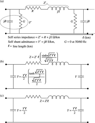
Figure 3.32 Representation of lines and cables: (a) distributed parameter circuit; (b) accurate π lumped parameter equivalent circuit and (c) nominal π lumped parameter equivalent circuit
Figure 3.32(c) is the nominal π lumped parameter equivalent circuit of the line or cable where the total impedance and susceptance are calculate by multiplying the per km parameters by the line/cable length. In Figure 3.32b, the terms in brackets represent correction terms that allow for the distributed nature of the circuit parameters over the entire circuit length. These terms can be represented as infinite series as follows:
 (3.142a)
 (3.142b)
The hyperbolic sine and tangent of a complex argument are equal to the complex argument itself when this has small values. For a lossless line or cable, the complex argument is equal to (2π/λ)l where λ is the wavelength in km and is given by λ; ≅ 3 × 10⁵/(f × ![]() ) where εr is the relative permittivity of the dielectric. For overhead lines (εr = 1 for air), the wavelength is approximately 6000 km at 50 Hz and 5000 km at 60 Hz. The definition of an ‘electrically short’ line or cable for which a nominal π circuit can be used depends on the acceptable error magnitude in the total series impedance and total shunt susceptance, and this determines the physical length in km for such a short line or cable. For an error of less than 1% in these parameters, the physical length should be less than about 3% of the wavelength. For overhead lines, this corresponds to 180 km for 50 Hz and 150 km for 60 Hz systems. For underground cables, with εr being typically between 2.4 and 4.2, the corresponding cable lengths using εr = 4.2 are 88 km for 50 Hz and 73 km for 60 Hz systems. In practice, these cable lengths are not reached above voltages of around 220 kV due to the adverse impact of the cable charging current on the cable thermal rating. For such lines or cables, the first term in the infinite series expansion of Equation (3.142), which is equal to unity, is taken and all other terms are neglected. Therefore, the exact equivalent π circuit of Figure 3.32(b) reduces to that shown in Figure 3.32(c).
) where εr is the relative permittivity of the dielectric. For overhead lines (εr = 1 for air), the wavelength is approximately 6000 km at 50 Hz and 5000 km at 60 Hz. The definition of an ‘electrically short’ line or cable for which a nominal π circuit can be used depends on the acceptable error magnitude in the total series impedance and total shunt susceptance, and this determines the physical length in km for such a short line or cable. For an error of less than 1% in these parameters, the physical length should be less than about 3% of the wavelength. For overhead lines, this corresponds to 180 km for 50 Hz and 150 km for 60 Hz systems. For underground cables, with εr being typically between 2.4 and 4.2, the corresponding cable lengths using εr = 4.2 are 88 km for 50 Hz and 73 km for 60 Hz systems. In practice, these cable lengths are not reached above voltages of around 220 kV due to the adverse impact of the cable charging current on the cable thermal rating. For such lines or cables, the first term in the infinite series expansion of Equation (3.142), which is equal to unity, is taken and all other terms are neglected. Therefore, the exact equivalent π circuit of Figure 3.32(b) reduces to that shown in Figure 3.32(c).
3.4.2 Sequence π models of single-circuit overhead lines and cables
Overhead lines
The PPS, NPS and ZPS impedances and susceptances of perfectly transposed single-circuit overhead lines were derived in Section 3.2.4. Recalling the sequence impedance and susceptance matrices of Equations (3.50a) and (3.54a), denoting 1 and 2 as the sending and receiving ends of the line or cable circuit and connecting 1/2 the susceptance at each end, as shown in Figure 3.33, we can write


and
 (3.143a)
For the PPS, NPS and ZPS circuits, the total injected current at ends 1 and 2 are given by
Therefore, using Equation (3.143), we obtain three separate PPS, NPS and ZPS sequence Π models for the line or cable as follows:
 (3.144)
As the PPS and NPS impedances and susceptances are equal, only two sequence Π models are needed as shown in Figure 3.32. For convenience, we will only refer to the PPS and ZPS sequence parameters and models in subsequent sections.
Cables
The sequence impedance matrices of single-circuit cables of various sheath earthing arrangements were derived in Section 3.3.4. The sequence impedance matrix of Equation (3.123), combined with the circuit sequence currents and voltages, gives
 (3.145)
The mutual intersequence terms are normally much smaller than the self-terms for solidly bonded cables and practically zero for cross-bonded cables. For the former, it is usual practice to ignore the mutual terms and use the self-terms only for the PPS, NPS and ZPS impedances of the cable. In the case of submarine cables where the three phases are laid a significant distance apart, the sequence impedance matrix is diagonal with no mutual intersequence terms. This is also the case for three-core cables, and single-core cables in touching trefoil or equilateral arrangements. The sequence susceptance matrix of all shielded and belted cables is diagonal and hence the PPS, NPS and ZPS susceptances are equal to the phase terms unaffected by any intersequence terms. Therefore, as in the case of single-circuit overhead lines, PPS and ZPS sequence Π models can be derived as shown in Figure 3.33.
3.4.3 Sequence Π models of double-circuit overhead lines
The PPS, NPS and ZPS impedances and susceptances of double-circuit overhead lines were derived in Section 3.2.6. We recall the sequence impedance and susceptance matrices of Equations (3.76a) and (3.78a) and illustrate their physical meaning as shown in Figure 3.34(a). Equation (3.76a) suggests that each circuit has a self PPS, NPS and ZPS impedance. In addition, PPS, NPS and ZPS inter-circuit mutual coupling exists between the PPS, NPS and ZPS impedances of each circuit. Importantly, we note that the three PPS, NPS and ZPS circuits are separate and independent. Equation (3.78a) contains similar information for susceptances. Allocating 1/2 the susceptances to each circuit end, Equations (3.76a) and (3.78b) of circuit 1 and circuit 2 are represented in Figure 3.34 as a Π model.

Figure 3.34 Double-circuit overhead line model in the sequence reference frame using sequence matrices: (a) schematic and (b) sequence π model
Using Figure 3.34 and Equations (3.76a) and (3.78a), we can write
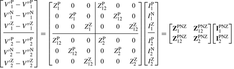


The equivalent admittance matrix can be derived for each sequence circuit independently because the PPS, NPS and ZPS circuits are separate. The form of the admittance matrix is the same for the PPS, NPS and ZPS circuits so the derivation of one would suffice. Collecting the PPS terms from Equation (3.146a), we have

saiyador
 (3.147a)
where ![]() . Similarly, collecting the shunt PPS terms from Equations (3.146b) and (3.146c), we have
. Similarly, collecting the shunt PPS terms from Equations (3.146b) and (3.146c), we have
 (3.147b)
The total injected currents into circuit 1 and circuit 2 at both ends are given by
 (3.148a)
Substituting Equations (3.147a) and (3.147b) into Equation (3.148a), we obtain
 (3.148b)
The NPS and ZPS admittance matrices of the double-circuit line with NPS and ZPS impedance and susceptance coupling between the two circuits are identical to that given in Equation (3.148b) except that the ZPS parameters are different.
The sequence model for a double-circuit overhead line derived above represents the case where the line is assumed to have had six transpositions. However, as we showed in Equation (3.89), when the line is assumed to be ideally transposed with nine transpositions, there would only be ZPS coupling between the two circuits. In this case, the ZPS admittance matrix would be identical to that of Equation (3.148b) but the PPS/NPS admittance matrices would have zero inter-circuit mutual impedances and susceptances as follows:
 (3.149)
3.4.4 Sequence Π models of double-circuit cables
As presented in Section 3.3.3, the series sequence impedance matrix of each cable circuit in a double-circuit cable will effectively be diagonal. There will also be inter-circuit mutual inductive coupling between the two circuits but the inter-circuit phase impedance mutual matrix is in general not balanced. For cross-bonded single-core double circuit cables, there would be very small intersequence mutual coupling between the two circuits in the PPS and NPS but a non-negligible coupling in the ZPS depending on spacing between the two circuits. The same applies for a three-core double-circuit cable. As presented in Section 3.3.4, the shunt sequence susceptance matrix of a single-circuit cable is diagonal, i.e. there is no intersequence mutual coupling. The presence of a second cable circuit has no effect other than introducing a second diagonal shunt sequence susceptance matrix for this circuit. Therefore, the PPS and ZPS sequence Π models shown in Figure 3.33 for a single-circuit cable may also be used for double-circuit cables. Where ZPS impedance coupling between the two cable circuits is significant and needs to be represented, then the approach described in Section 3.4.3 for double-circuit overhead lines can be used.
3.5 Sequence π models of three-circuit overhead lines
Using a similar approach to that of Section 3.4.3, Figure 3.35 illustrates three mutually coupled circuits and their self and mutual sequence impedance and susceptance matrices.

Figure 3.35 Three-circuit overhead line model in the sequence reference frame: (a) schematic and (b) ZPS π model
The sequence Π model represents either the PPS, NPS or ZPS equivalent circuits. Where ideal transposition is used with only ZPS inter-circuit mutual coupling, the PPS and NPS Π model of each circuit is completely independent from the other circuits. We will now derive the admittance matrix for the general case where inter-circuit mutual coupling exists and we will use the ZPS Π model parameters but drop the superscript Z to simplify notation.
From Figure 3.35(b), we can write

or
 (3.150a)
 (3.150b)
The total injected currents into each circuit at both ends are given by
 (3.151)
or written in concise matrix form using Equation (3.150a), we have

or
 (3.152a)
where
 (3.152b)
3.6 Three-phase modelling of overhead lines and cables (phase frame of reference)
3.6.1 Background
In advanced studies such as multiphase loadflow and short-circuit fault analysis where the natural unbalance of untransposed lines and cables is to be taken into account, the modelling and analysis may be carried out in the phase frame of reference. Such analysis allows the calculation of the current distribution on overhead line earth wires and cable sheaths under unbalanced power flow and short-circuit faults.
3.6.2 Single-circuit overhead lines and cables
For single-circuit overhead lines, the series phase impedance matrices with earth wires present and eliminated were given in Equations (3.29) and (3.32c), respectively. The corresponding shunt phase susceptance matrices are obtained from the inverse of Equation (3.36) and from Equation (3.39). Considering the case of an overhead line with one earth wire, the line can be represented by a three-phase equivalent nominal Π model as shown in Figure 3.36(a).

Figure 3.36 Three-phase model of a single-circuit line including earth wire(s): (a) Π equivalent circuit and (b) π model (matrices)
In Figure 3.36, the line is represented by its series phase impedance matrix and 1/2 its shunt phase susceptance matrix connected at each end. We denote as 1 and 2 the two ends of the line, and we use ‘ph’ for ‘phase’ quantities, which also include the earth wires if these have not been eliminated. From Figure 3.36(b), we have
Therefore, the nodal phase admittance matrix is given by
 (3.153b)
If the earth wire has already been eliminated, then it is simply removed from Figure 3.36(a) and the dimension of the series phase impedance and shunt phase susceptance matrices is reduced accordingly. The series phase impedance and shunt phase admittance matrices for cables, with their sheaths present or eliminated, can be represented using a similar approach taking into account the particular sheath earthing arrangement. Figure 3.37 shows a three-phase model for a single-circuit underground cable with a solidly bonded sheath.

3.6.3 Double-circuit overhead lines and cables
For double-circuit overhead lines, the series phase impedance matrices with earth wires present and eliminated are given in Equations (3.57a) and (3.58b), respectively. The corresponding shunt phase susceptance matrices are obtained from the inverse of Equation (3.60a) and (3.62c), respectively. Using the π matrix model shown in Figure 3.36(b) together with the inter-circuit mutual impedance and susceptance matrices, we obtain the π model representation of a double-circuit overhead line in the phase frame of reference as shown in Figure 3.38.

Figure 3.38 Three-phase model of a double-circuit line including earth wire(s): (a) π equivalent circuit and (b) π model (matrices)
We denote 1 and 1′, and 2 and 2′ as the two ends of circuit 1 and circuit 2, respectively. We assume that the inter-circuit mutual coupling is bilateral, i.e. B21 = Bt12. From Figure 3.38, the series voltage drop across the two circuits is given by

or
 (3.154)
The shunt susceptance currents are given by
 (3.155)
Since the total current injected into each circuit end is the sum of the series and shunt currents, it can be shown that the nodal phase admittance matrix equation of the mutually coupled double-circuit line is given by
 (3.156)
All quantities in Equation (3.156) are matrices. Where the earth wires are eliminated, the dimensions of the impedances and susceptances are 3 × 3 and those of the current and voltage vectors are 3 × 1. Therefore, the dimension of the nodal current and voltage vectors are 12 × 1 and the dimension of the admittance matrix of the double-circuit line is 12 × 12. The same approach presented above can be followed in the case of double-circuit cables although the dimensions of the matrices will be increased to a greater extent by the number of sheaths and armours as appropriate.
3.7 Computer calculations and measurements of overhead line and cable parameters
3.7.1 Computer calculations of overhead line and cable parameters
The days of hand or analytical calculations of overhead line and cable phase and sequence impedances and susceptances have long gone together with, unfortunately, some of the great insight such methods provided. The calculations of overhead line and cable electrical parameters at power frequency, i.e. 50 or 60 Hz, as well as higher frequencies, are nowadays efficiently carried out using digital computer programs. For overhead lines, the input data are phase conductor and earth wire material and resistivity, physical dimensions, dc or ac resistance, conductor bundle data, tower geometry, i.e. spacing between conductors and conductor height above ground, average conductor sag and earth resistivity. The output information usually comprises the line’s ac resistance matrix, inductance matrix, series phase reactance matrix, series phase impedance matrix, potential coefficient matrix, shunt capacitance matrix and shunt susceptance matrix, all including and excluding the earth wires. Assumptions of phase transpositions can be easily implemented using efficient matrix analysis techniques. The sequence data calculated consists of the series sequence impedance and shunt sequence susceptance matrices. The dimension of these sequence matrices is 3N where N is the number of three-phase circuits. The output information is usually calculated in physical units, e.g. μF/km/phase or ω/km/phase and in pu or % on some defined voltage and MVA base.
For cables, the input data are core, sheath and, where applicable, armour conductor material and resistivity, their physical dimensions, dc or ac resistance, the cable layout or spacing between phases, relative permittivity of core, sheath and, where applicable, armour insulation, as well as earth resistivity. The output information usually comprises the cable’s full and reduced series phase impedance shunt susceptance matrices, i.e. including and excluding the sheaths and armour(s). The sequence data calculated consists of the sequence series impedance matrix and sequence shunt susceptance matrix.
3.7.2 Measurement of overhead line parameters
General
Measurements of overhead lines power frequency electrical parameters or constants can be made at the time of commissioning when the line construction has been completed so that the tests replicate the line in normal service operation. The parameters that may be measured are phase conductor self and mutual impedances with earth return, and self and mutual susceptances. The series phase impedance and shunt phase susceptance matrices are then constructed and the sequence impedances and susceptances calculated. There are numerous designs of overhead lines used in practical installations but we will illustrate the techniques that can be used for single-circuit line with one earth wire and double-circuit line with one earth wire. The technique can be extended for application to any other line construction.
Single-circuit overhead lines with one earth wire
Figures 3.39(a) illustrates a technique for phase impedance measurements where the three-phase conductors are earthed at the far end of the line but kept free from earth at the near measurement end.

Figure 3.39 Measurement of the electrical parameters of a single-circuit overhead line: measurement of self and mutual (a) series phase impedances with earth return and (b) shunt phase susceptances
A test voltage is applied to one-phase conductor and the current flowing through it is measured. The induced voltages to earth on the remaining conductors are also measured. In addition to the calculation of the impedances from the measured voltages and currents, a wattmeter or phase angle meter can be used to find the phase angle of these voltages with respect to the injected current. This allows the calculation of the resistance and reactance components of the impedance using R = P/I2 (P is measured phase power in Watts) and X = ![]() in the case of a wattmeter, but R = Z × cos φ and X = Z × sin φ in the case of a phase angle meter measurement. The process is repeated for all other conductors. Where earth wire(s) are present, the measured impedances should represent values with the earth wire in parallel with earth return path to represent normal service operation.
in the case of a wattmeter, but R = Z × cos φ and X = Z × sin φ in the case of a phase angle meter measurement. The process is repeated for all other conductors. Where earth wire(s) are present, the measured impedances should represent values with the earth wire in parallel with earth return path to represent normal service operation.
Using the single-circuit phase impedance matrix including the effect of earth wire that is with the earth wire mathematically eliminated, we have
With the voltage source applied to conductor 1, V1 is known and the measured values are I1, V2 and V3 with I2 = I3 = 0. Using the measured values in Equations (3.157), we obtain
Applying the voltage source to conductor 2 then conductor 3, we obtain
For sequence impedance calculations, and with the line assumed to be perfectly transposed, the self and mutual impedances per phase are calculated as the average of the measured self and mutual impedances as follows:
and
Therefore, the PPS and ZPS impedances are given by
Figure 3.39(b) illustrates a technique for phase susceptance measurements where the three-phase conductors are earthed through milliammeters at the near measurement end of the line but kept free from earth, i.e. open circuit at the far end. A test voltage is applied in series with one-phase conductor and the currents flowing through all conductors are measured. The process is repeated for all other conductors. As in the case of impedance measurements the measured susceptances should include the effect of the earth wire. Using the single-circuit phase susceptance matrix including the effect of earth wire that is with the earth wire mathematically eliminated, we have
With the test voltage source applied to conductor 1, V1 is known and the measured values are I1, I2 and I3 with V2 = V3 = 0. Using the measured values in Equations (3.161), we obtain
Applying the test voltage source to conductor 2 then conductor 3, we obtain
and
For sequence susceptance calculations and with the line assumed to be perfectly transposed, the self and mutual susceptances perphase are calculated as the average of the measured self and mutual susceptances as follows:
and
Therefore, the PPS and ZPS impedances are given by
The measured voltages and currents inherently take into account the distributed nature of the line’s impedances and susceptances. However, we have used lumped linear impedance and susceptance matrix models for the line which will introduce small errors in the calculated impedances and susceptances depending on line length. The calculated impedances and susceptances can be corrected for the line length effect if the equivalent Π circuit of a distributed multi-conductor line derived in Appendix 1 is used. The impedance and susceptance constants now become impedance and susceptance matrices and the general nodal admittance equations for a multi-conductor line are given by
and IS and IR are the line’s sending and receiving end current vectors, respectively; and VS and VR are the line’s sending and receiving end voltage vectors, respectively.
In the impedance measurement technique, the voltage and current vectors VS and IS are known from the measurements, VR = 0 but IR is unknown. Therefore, from Equation (3.165), we can write ![]() Expanding the hyperbolic tangent into an infinite series, we obtain
Expanding the hyperbolic tangent into an infinite series, we obtain
In the susceptance measurement technique, the voltage and current vectors VS and Is are known from the measurements, IR = 0 but VR is unknown. Therefore, from Equation (3.165), we can write ![]() Using the values of A and B from Equation (3.165) and expanding the hyperbolic tangent into an infinite series, we obtain
Using the values of A and B from Equation (3.165) and expanding the hyperbolic tangent into an infinite series, we obtain
We can use the voltages and currents obtained from the test measurements to calculate to a first approximation of the elements of the impedance and susceptance matrices using the approximate lumped parameter equations as follows:
Z1 and Y1 can now be equated to the series impedance and susceptance values of Equations (3.166) and (3.167) and used to obtain a second approximation as follows:
Similarly, the new values of the impedance and susceptance matrices can again be used to obtain an improved approximation and the process can be repeated until the desired level of accuracy is obtained. In general, we can write
Double-circuit overhead lines
The technique presented above for a single-circuit overhead line with one earth wire can be extended to double-circuit overhead lines with any number of earth wires. Figure 3.40 shows the impedance and susceptance test arrangements.

Figure 3.40 Measurement of electrical parameters of a double-circuit overhead line: measurement of self and mutual (a) series phase impedances with earth return and (b) shunt phase susceptances
The measured phase impedance and susceptance matrices are given as

 (3.171b)
In Figure 3.40(a), we apply a voltage source V1 to conductor 1 and measure I1, V2, V3, V4, V5 and V6. In Figure 3.40(b), we apply a voltage source V1 to conductor 1 and measure I1, I2, I3, I4, I5 and I6. From these tests, and using Equation (3.171), the self and mutual phase impedances and susceptances are calculated as follows:
 (3.172b)
In both impedance and susceptance tests, the voltage source is applied to each phase conductor in turn in order to measure all the self and mutual impedances and susceptances of Equation (3.171). The balanced phase and resultant sequence impedances can be calculated assuming an appropriate number of phase transpositions such as three, six or ideal nine transpositions. The reader is encouraged to derive the balanced phase and sequence parameters. The sequence susceptance parameters can be similarly calculated.
3.7.3 Measurement of cable parameters
General
Measurements of power frequency electrical parameters or constants of cables can be made at the time of commissioning when the cable installation has been completed so that the tests replicate the cable in normal service operation. The relevant parameters that are usually measured are the conductor dc resistances at prevailing ambient temperature, the PPS/NPS and ZPS impedances and sometimes the PPS/NPS/ZPS susceptances. As there are numerous designs and layouts of cables in use in practical installations, we will illustrate the techniques that can be used for a typical single-circuit single-core three-phase coaxial cable with core and sheath conductors. An illustration of the PPS/NPS susceptance and ZPS susceptance measurement of a three-core belted cable is also presented.
Measurement of dc resistances
The dc resistances of the cores and sheaths (screens) are measured using a dc voltage source as illustrated in Figure 41.3(a) and (b). In the first case, the dc voltage source V is applied between cores 1 and 2 with the third core floating and remote ends of the three cores short-circuited. The dc source V is next applied between cores 1 and 3, then 2 and 3. The measured core loop resistance in each case is calculated from RCc(loop) = V/I and the three measured loop resistances are given by
Therefore, the individual core resistances are given by
The test procedure for the sheath or screen dc resistances is similar to that for the core dc resistances but the dc voltage source is now applied between two sheaths at a time as shown in Figure 3.41(b).

Measurement of PPS/NPS impedance
The measurement of the cable’s PPS/NPS impedance per phase requires a three-phase power frequency source. On each of the single cores, measurements of voltage, current and phase power or phase angle are made. The sheath’s bonding and earthing must correspond to that in actual circuit operation. Figure 3.42(a) illustrates the PPS/NPS impedance measurement for a cable with a sheath that is solidly bonded at both ends. From the measurements, the following calculations for each phase are made.

If a wattmeter is used to measure input power, we have
If a phase angle meter is used to measure the angle between the input voltage and current
where PP is the measured phase power in Watts. The three values obtained for each phase are then averaged and this is particularly important in the case of untransposed cable systems. The final PPS/NPS cable parameters are given as
 (3.176)
Measurement of ZPS impedance
The measurement of the cable’s ZPS impedance per phase requires a single-phase power frequency source. The three cores at the test end are bonded together and at the remote end are bonded together and to the sheaths. Single-phase currents are injected into the cable cores to return via the sheath and earth. Figure 3.42(b) illustrates the test circuit. The sheaths are solidly bonded at both ends as in actual cable operation. The calculations of the ZPS impedance, resistance and reactance use similar equations to those used for the PPS/NPS impedance except that the current should now be divided by 3, i.e. the impedance equation becomes
Measurement of earth loop impedances
As in the case of an overhead line, and if required, the earth loop impedances for each core and sheath may also be measured using a single-phase power frequency source. The technique is similar to that presented in Section 3.7.2.
Measurement of PPS/NPS/ZPS susceptance
The measurement of a screened cable core-to-sheath, and if required, sheath-to-earth susceptances uses a single-phase power frequency source. The three cores at the remote end are left floating, i.e. open circuit. The applied voltage V, charging current I and phase angle φ between applied voltage and current, the latter measured using a low power factor meter, are measured. This is usually called the power factor and capacitance test of the dielectric. The calculations made are
B is the PPS/NPS/ZPS susceptance per phase. G is very small and is usually neglected in power frequency steady state analysis.
For three-core belted cables, the core-to-core and core-to-sheath capacitances can be calculated from two measurements. The core to sheath, i.e. ZPS susceptance can be measured by short-circuiting the three cores and applying a voltage source V between them and the earthed sheath, see Figure 3.29(c). From the measured injected current I, we can write
The core-to-core capacitance can be obtained from a measurement where a voltage source V is applied between two cores with the third core short-circuited to the sheath. Let the measured susceptance be BMeas. Therefore, using Figure 3.29(c), we can write
Therefore, the core-to-core susceptance is calculated as
Using Equation (3.138c), the PPS susceptance of the cable is given by
3.8 Practical aspects of phase and sequence parameters of overhead lines and cables
3.8.1 Overhead lines
During the installation and commissioning of new overhead line designs, it was common practice to carry out field test measurements of the phase self and mutual impedances and susceptances. From these tests, the sequence impedances and susceptances are obtained. Measurements of sequence parameters could also be made. Measurements served as benchmark values for the validation of line’s power frequency models and calculations carried out on digital computers. The range of errors in the calculations of the sequence impedance parameters is usually very small. The assumption of conductor temperature used in the calculation is important primarily for resistance calculation and to a small extent reactance and susceptance calculations due to changes in conductor sag. Also, a reasonable value of uniform earth resistivity may be used and this may be an average value to represent the route over which the line runs. In England and Wales and in America, average uniform earth resistivities of 20 and 100 ωm are generally used.
3.8.2 Cables
For cables, available models and computer calculations of the PPS/NPS impedances and sequence susceptances usually provide results with good accuracy in comparison with field test measurements despite the large variety of cable designs and installations. However, this is not normally the case for the ZPS impedance particularly for high voltage cables. In addition to the cable design including its sheath or screen and cable layout, the ZPS impedance strongly depends on any other local and nearby metal objects that may form a return path in parallel with the cable sheath itself. These might be other parallel cables, nearby water pipes and pipelines, gas mains, subway structures, railway tracks and lines, steel or concrete tunnels and any earth electrodes that may be used, etc. The information about most of these additional factors is practically unknown and impossible to obtain so they cannot be appropriately included in the calculation. The only practical solution to obtain accurate results is to carry out field test measurement of the ZPS impedance with the cable installed as in actual service operation. In addition, such a measurement will only be accurate at the time it is taken but it may be different a few years later. This may be caused by underground construction or modifications of conducting material e.g. water and gas mains.
[1] Bickford J.P., et al. Computation of Power-System Transients. Peter Peregrinus Ltd.; 1980. 0-906048-35-4.
[2] ISBN 0-246-11467-3McAllister D. Electric Cables Handbook, Granada. 1982.
[3] Library of Congress catalog card number: 65-122253Abramowitz M., Stegun I., et al. Handbook of Mathematical Functions. Dover publications, Inc.; 1964.
[4] IEC 60287-1-3, Electric Cables-Calculation of Current Rating, 1st Edn 2002–2005.
[5] Carson J.R. Wave propagation in overhead wires with ground return. Bell System Technical Journal. 1926;Vol. 5:539-554.
[6] Pollaczek F. Ueber das feld einer unendlich langen wechsel stromdurchflossenen einfachleitung. Elektrische Nachrichten Technik. 1926;Vol. 3(No. 5):339-359.
[7] Schelkunoff S.A. The electromagnetic theory of coaxial transmission lines and cylindrical shells. Bell System Technical Journal. 1934;Vol. XIII:532-578.
[8] Haberland G. Theorie der Leitung von Wechselstrom durch die Erde. Zeitschrifi fir Angewand te Mathematic and Mechanik. 1926;Vol. 5(No. 6):366.
[9] No. 6Wang Y.J. A review of methods for calculation of frequency-dependent impedance of overhead power transmission lines. Proceedings of the National Science Council Republic of China(A). Vol. 25. 2001:329-338.
[10] Galloway R.H., et al. Calculation of electrical parameters for short and long polyphase transmission lines. Proceedings IEE. Vol. 111. December 1964:2051-2059.
[11] Dommel H.W. Overhead line parameters from handbook formulas and computer programs. IEEE Transactions on PAS. February 1985;Vol. PAS-104(No. 2):366-372.
[12] Nielsen H., et al. Underground Cables and Overhead Lines Earth Return Path Impedance Calculations with Reference to Single Line to Ground Faults. Denmark: Aalborg University; 2004:1-11.
[13] Ametani A. A general formulation of impedance and admittance of cables. IEEE Transactions on PAS. May/June 1980;Vol. PAS-99(No. 3):902-910.
[14] Brown G.W., et al. Surge propagation in three phase pipe-type cables, Part 1_unsaturated pipe. IEEE Transactions on PAS. January/February 1976;Vol. PAS-95(No. 1):89-95.
[15] Bianchi G., et al. Induced currents and losses in single-core submarine cables. IEEE Transactions on PAS. January/February 1976;Vol. PAS-95(No. 1):49-58.
[16] No. 2Wedepohl L.M., et al. Transient analysis of underground power-transmission systems. IEE Proceedings. Vol. 120. February 1973:253-260.