
4 Modelling of transformers, static power plant and static load
4.1 General
In this chapter, we describe modelling techniques of various types of transformers, quadrature boosters (QBs), phase shifters (PSs), series and shunt reactors, series and shunt capacitors, static variable compensators and static power system load. Sequence, i.e. positive phase sequaence (PPS), negative phase sequence (NPS) and zero phase sequence (ZPS) models, as well as three-phase models suitable for analysis in the phase frame reference are presented. Sequence impedance measurement techniques of transformers, QBs and PSs are also described.
4.2 Sequence modelling of transformers
4.2.1 Background
The invention of the transformer machine towards the end of the nineteenth century having the basic function of stepping up or down the voltages (and currents but in opposite ratios) created the advantage of transmitting alternating current (ac) electric power over larger distances. This was not possible with direct current (dc) electric power since the locations of power generation and demand centres could not be too far apart. This is to ensure that power loss and voltage drops are kept to a reasonably low level. The technology of transformers has undergone significant developments during the twentieth century and many types of transformers are nowadays used in ac power systems.
Three banks of single-phase transformers are generally used in power stations to connect very large generators to transmission networks with the low voltage (LV) and high voltage (HV) windings connected as required, e.g. in delta or star. The main reasons for using separate banks are to reduce transport weight, improve overall transformer availability and reliability, and reduce the cost of spare holding. Single-phase transformers are also used in remote rural distribution networks to supply small single-phase demand consumers where three-phase supplies are uneconomic to use. There are also special applications where single-phase transformers are used such as in the case of high capacity traction transformers connected to three-phase power networks, usually connected to two phases of the three-phase transmission or distribution network. Other applications of single-phase transformers are those used to provide neutral earthing for generators.
Three-phase power transformers are invariably used in transmission, subtransmission and distribution substations for essentially voltage transformation. In addition, they are also used for voltage or reactive power flow control and active power flow control. For the latter application, they are called PS or QB transformers. Other applications of three-phase power transformers are for connections to converters in high voltage direct current (HVDC) links, for earthing of isolated systems, as well as in large industrial applications such as arc furnaces.
Transformers used for voltage control are equipped with off-load or on-load tap-changers that vary the number of turns on the associated winding and hence the turns ratio of the transformer. In some countries, e.g. the UK, generator transformers are generally equipped with on-load tap-changers on the HV winding with the HV side voltage being the controlled voltage. Typical voltage transformations are 11–142 kV, 15–300 kV and 23.5-432 kV. Two-winding transformers having large transformation ratios may be equipped with on-load tap-changers on the HV winding but with the LV winding voltage being the controlled voltage. Typical transformations are 275–33 kV, 132–11 kV, 380–110 kV and 110–20 kV. Distribution transformers, e.g. 11–0.433 kV usually have off-load tap-changers.
Where the transformation ratio is generally less than about three, e.g. 400 kV/132 kV and 500 kV/230 kV, autotransformers are generally more economic to use. Nowadays with increased trends towards automation, autotransformers that supply power to distribution systems tend to be equipped with on-load tap-changers. These may be located either at the LV winding line-end or neutral-end with the LV winding voltage being the controlled voltage. Autotransformers may also have a third low MVA capacity delta-connected winding called ‘tertiary’ winding. These may be used for the connection of reactive compensation plant e.g. capacitors, reactors or synchronous compensators (condensers). They also provide a path for the circulation of triplen harmonic currents and hence prevent or reduce their flow on the power network as well as reduce network voltage unbalance.
The calculation of unbalanced currents and voltages due, for example, to short-circuit faults requires correct and practical modelling of power transformers. In this section, we present the theory of modelling single-phase transformers, and three-phase power transformers having various numbers of windings and different types of winding connections. Knowledge of basic electromagnetic transformer theory is assumed. Figures 4.1 and 4.2 show two large autotransformers used in a 400 kV/275 kV/132 kV transmission system.


4.2.2 Single-phase two-winding transformers
The power transformer is a complex static electromagnetic machine with windings and a non-linear iron core. We will first present the transformer equivalent circuit in actual physical units then derive the per-unit equivalent circuit for the cases where the transformer has nominal and off-nominal turns ratios. The latter corresponds to the common case where the transformer is equipped with an on-load tap-changer.
Equivalent circuit in actual physical units
The conventional equivalent circuit of a single-phase two-winding transformer is shown in Figure 4.3(a).

Figure 4.3 Single-phase transformer equivalent circuit in actual physical units: (a) basic equivalent circuit and (b) L winding impedance referred to H winding
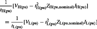
Where all quantities shown are in physical units of volts, amps and ohms, and ZH = RH + jXH, RH = HV winding resistance, XH = HV winding leakage reactance. ZL = RL + jXL, RL = LV winding resistance, XL = LV winding leakage reactance. RI = resistance representing core iron losses which are assumed to vary with the square of applied HV winding voltage. XM = core magnetising reactance referred to the HV side and representing the rms value of the magnetising current. NH and NL are the actual number of turns of HV and LV windings, respectively. NH(nominal) and NL(nominal) are HV and LV winding number of turns at nominal tap positions, respectively.
From basic transformer theory and since the same flux will thread both HV and LV windings, the induced voltage per turn on the HV and LV windings are equal, hence
In the derivation of the equivalent circuit, we will initially neglect the ampere-turns or MMF due to the exciting shunt branch that represents the very small core iron and magnetising losses. The HV winding and LV winding MMFs, for the current directions shown in Figure 4.3(a) are related by
Also, the voltage drop equations for the transformer HV and LV windings can be written as follows:
Using Equations (4.1a) and (4.2b), Equation (4.2a) can be rewritten as
Substituting Equation (4.1b) into Equation (4.3), we have
ZHL is the equivalent transformer leakage impedance referred to the HV side and ![]() is the LV impedance referred to the HV side. Figure 4.3(b) is drawn using Equation (4.4a) ignoring the shunt exciting branch. The LV voltage VL and LV current IL are referred to the HV side as NVHVL and IL/NHL, respectively. The exciting shunt branch can be reinserted between
is the LV impedance referred to the HV side. Figure 4.3(b) is drawn using Equation (4.4a) ignoring the shunt exciting branch. The LV voltage VL and LV current IL are referred to the HV side as NVHVL and IL/NHL, respectively. The exciting shunt branch can be reinserted between ![]() on the input HV terminals. Alternatively, ZH could have been referred to the LV side and the exciting branch inserted similarly. The exciting impedance is much bigger than the leakage impedances of either winding by almost a factor of 400–1. However, modern short-circuit, power flow and transient stability analyses practice includes the iron loss branch as well as the magnetising branch.
on the input HV terminals. Alternatively, ZH could have been referred to the LV side and the exciting branch inserted similarly. The exciting impedance is much bigger than the leakage impedances of either winding by almost a factor of 400–1. However, modern short-circuit, power flow and transient stability analyses practice includes the iron loss branch as well as the magnetising branch.
Equivalent circuit in per unit
In many types of steady state analysis, we are interested in the transformer equivalent circuit where all quantities are in per unit on some defined base quantities. Let the base quantities be defined as
 (4.5a)
In Equation (4.5b), the HV and LV windings’ nominal tap positions are chosen to correspond to the HV and LV base voltages of the network sections to which the windings are connected.
Let us now define the following per-unit quantities:
Dividing Equation (4.3) by S(B) and using Equations (4.5) and (4.6), we obtain

which can be rewritten as
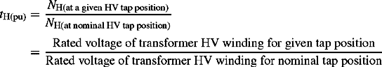
where the pu tap ratios of the HV and LV windings are given by
and
We will now assume that the impedance of each winding is proportional to the square of the number of turns of the winding. We know from basic transformer theory that this is generally valid for the winding inductive reactance but not for the winding resistance. However, because the resistance is generally much smaller than the reactance, this approximation is accepted. Thus, we define ZH(nominal) as the pu HV winding impedance at nominal HV winding tap position and ZL(nominai) as the pu LV winding impedance at nominal LV winding tap position. Therefore, for each winding, we have
Substituting Equation (4.8) into Equation (4.7a), we obtain
 (4.9)
(4.9)The general pu equivalent circuit shown in Figure 4.4(a) represents Equation (4.9).

Figure 4.4 Transformer equivalent circuits in pu: (a) pu equivalent circuit of general off-nominal-ratio transformer; (b) pu equivalent circuit with H side off-nominal ratio; (c) pu equivalent circuit with L side off-nominal ratio and (d) pu equivalent circuit of nominal-ratio transformer
In practice, we are more interested in deriving an equivalent where both impedances appear on one side of the ideal transformer. This can be done once we have derived the relationship between the HV and LV pu currents from Equation (4.1b) as follows:
which, using Equation (4.5b), can be written as
or, using Equations (4.7b) and (4.7c), reduces to
Substituting Equation (4.10) into Equation (4.9) and rearranging, we obtain the following two equations
and
where
 (4.11e)
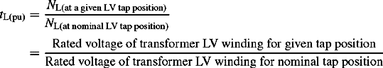 (4.11f)
Figure 4.4(b) and (c) represent Equations (4.11a) and (4.11b), respectively. Both equivalents are identical in terms of representing the general equivalent circuit of an off-nominal ratio transformer. However, in practice, it is more convenient to use one or the other depending on the actual transformer characteristics. That is, Figure 4.4(b) would be used to represent a transformer with the following characteristics:
(a) The HV side is equipped with an on-load tap-changer and the LV side is fixed nominal or fixed off-nominal ratio.
(b) The HV side is fixed off-nominal ratio and the LV side is fixed nominal ratio or fixed off-nominal ratio.
Figure 4.4(c), however, would be used to represent a transformer with the following characteristics:
(a) The LV side is equipped with an on-load tap-changer and the HV side is fixed nominal or fixed off-nominal ratio.
(b) The LV side is fixed off-nominal ratio and the HV side is fixed nominal ratio or fixed off-nominal ratio.
We will make a number of important practical observations that apply to Figure 4.4(b) and (c). Considering Figure 4.4(b), and in the case of a tap-changer located on the HV winding with a fixed nominal or off-nominal ratio on the LV winding, then only tH changes but ZLH does not change with HV tap position. Similar observation applies to Figure 4.4(c). In both circuits, the variable tap ratio of the ideal transformer, tHL or tLH, is located on the side equipped with the on-load tap-changer. That is, it is located away from the transformer impedance which has a value that correspond to the fixed nominal or off-nominal ratio of the other side. It should be noted that the location of the variable tap ratio is a purely arbitrary choice and it could have been placed on the impedance side provided that Equations (4.11a) and (4.11b) continue to be satisfied.
A nominal-ratio-transformer is one where the chosen base voltages of the network sections to which the transformer is connected are the same as the transformer turns ratio or rated voltages. For such a transformer, Equation (4.7) reduces to tH = 1 and tL = 1, hence the ideal transformers shown in Figure 4.4(b) and (c) can be eliminated as shown in Figure 4.4(d).
However, for many transformers used in power systems, the transformer voltage ratio is not the same as the ratio of base or rated voltages of the associated network sections. Therefore, the choice of voltage base quantities for the network has to be made independent of the transformer actual voltage ratio or turns ratio. The most common reason for this is that a very large number of transformers used in power systems are equipped with tap-changers, on the HV or LV winding, whose function is to vary the number of turns of their associated winding. In addition, some distribution transformers, in particular, can have one winding with a fixed off-nominal ratio.
To ensure a proper understanding of the concepts introduced in deriving Figure 4.4, we will present a number of practical cases. In the first case, consider a single-phase 11 kV/0.25 kV distribution transformer interconnecting an 11 kV network and a 0.25 kV network. The transformation ratio or turns ratio of 11–0.25 kV corresponds exactly to the network base voltages. Therefore, Figure 4.4(d) represents such a transformer. We also note that with the transformer on open circuit, VH(pu) = VL(pu) but with the transformer on-load, IH(pu) = −IL(pu).
In the second case, we consider a 10 kV/0.25 kV single-phase transformer interconnecting an 11 kV network and a 0.25 kV network. The HV winding is clearly a fixed off-nominal-ratio winding. The pu tap ratio tHL in Figure 4.4(b) is calculated as
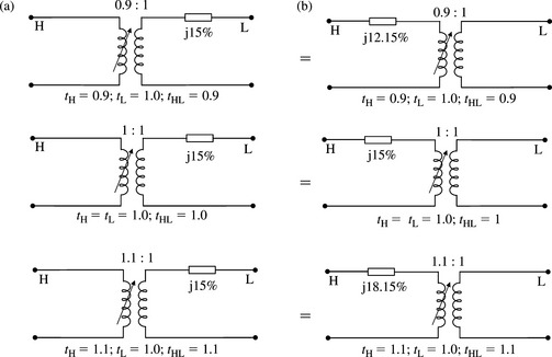
In the third case, we consider a transformer equipped with an on-load tap-changer on the HV side and we will also consider the effect on the transformer impedance. Consider a 239 MVA, 231 kV/21.5 kV single-phase transformer (this is actually one of a 717 MVA, 400 kV/21.5 kV three-phase bank) having a nominal-ratio leakage reactance of 15% on rating (the resistance is ignored for the purposes of this example but not in practical calculations). The transformer is connected to a network with 231 and 21.5 kV base voltages. The transformer, therefore, has a fixed LV nominal-ratio, i.e. tL = 1. The tap-changer is located on the 231 kV winding hence tH is variable. We will calculate the transformer reactance and redraw the equivalent circuit of Figure 4.4(b) to correspond to the transformation ratios 207.9 kV/21.5 kV, 231 kV/21.5 kV and 254.1 kV/21.5 kV The three voltage transformation ratios correspond to tH values of 0.9, 1.0 and 1.1, respectively. Clearly, the transformer impedance value does not change from nominal as illustrated in Figure 4.5(a). It is instructive for the reader to demonstrate that if the tap ratio is placed on the impedance side, then, by making appropriate use of Figure 4.4(c), the reactance values that correspond to tH = 0.9, 1.0 and 1.1 would become 12.15%, 15% and 18.15%, respectively. This is illustrated in Figure 4.5(b). The reader should also demonstrate that the corresponding circuits of Figure 5.4(a) and (b) are equivalent to each other. This can be done by calculating, for the corresponding equivalent circuits, the short-circuit impedances, i.e. the impedance seen from one side, e.g. H side with the other side, L side, short-circuited and vice versa. The calculated impedances will be identical.
The variation of the tap position of a transformer equipped with an on-load tap-changer results in a value of tHL, for most transformers used in electric power systems, to be generally within 0.8 and 1.2 pu.
π Equivalent circuit model
The ideal transformer in the general pu equivalent circuit of an off-nominal-ratio transformer shown in Figure 4.4(b) and (c) is, although suitable for use on network analysers, not satisfactory for modern calculations that are almost entirely based on digital computation. Therefore, the ideal transformer must be replaced with a suitable equivalent circuit and this will be achieved by deriving an equivalent π circuit model for Figure 4.4(b). The reader is encouraged to do so for Figure 4.4(c). For convenience, we will drop the explicit pu notation and recall that all quantities are in pu. From Figure 4.4(b), we can write
or
also
or
or in matrix form
 (4.13a)
The admittance matrix of Figure 4.4(c) can be similarly derived and the result is
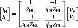 (4.13b)
The equations of the general equivalent π circuit shown in Figure 4.6(a) are

Figure 4.6 π equivalent circuit of an off-nominal-ratio transformer: (a) general π equivalent circuit, (b) π equivalent circuit of Figure 4.4(a) and (b) π equivalent circuit of Figure 4.4(c)
or in matrix form
 (4.14c)
Equating the admittance terms in Equations (4.13a) and (4.14c), we have
and
and
Similarly, equating the admittance terms in Equations (4.13b) and (4.14c), we have
and
and
The equivalent π circuit models of the off-nominal-ratio transformer of Figure 4.4(b) and (c) are shown in Figure 6.4(b) and (c), respectively. The equivalent K circuit model parameters for the three conditions shown in Figure 4.5(a) are calculated and shown in Figure 4.7. Also shown in Figure 4.7 are the short-circuit impedances calculated from side H with side L short-circuited, and vice versa. It should not come as a surprise to the reader that these impedances are identical to the ones that the reader may have calculated, as recommended previously, for the equivalent circuits shown in Figure 5.4(a) and (b).

As mentioned before, it is generally no longer the case in modern industry practice to neglect the shunt exciting branch representing the iron losses and magnetising losses. The exciting branch admittance can be calculated from the corresponding impedance and inserted in parallel with either YB or YC or it can also be inserted as a shunt admittance midway through the series impedance. There is also a usual approximation to split it in half and connect each half at either end of the equivalent circuit. The admittance of the exciting or magnetising branch is given by
The general 2 × 2 admittance matrix is given by
 (4.17a)
whose elements, using Equation (4.15), are given by
whereas, using Equation (4.16), the matrix elements are given by
4.2.3 Three-phase two-winding transformers
The majority of power transformers used in power systems are three-phase transformers since these have significant economic benefits compared to three banks of single-phase units that have the same total rating and perform similar duties. On the other hand, reliability considerations for very large three-phase transformers may result in the use of three banks of single-phase units. In double-wound transformers, there is a low voltage winding and an electrically separate high voltage winding.
Winding connections
In three-phase double-wound power transformers, the three-phases of each winding are usually connected as star or delta. There are thus four possible connections of the primary and secondary windings namely star–star, star–delta, delta–star and delta–delta connections. Interconnected star or zig–zag windings are dealt with in Section 4.2.6.
PPS and NPS equivalent circuits
Like all static three-phase power system plant, the impedance such plant presents to the flow of PPS or NPS currents is independent of the phase rotation or sequence of the three-phase applied voltages R, Y, B or R, B, Y. Therefore, the plant PPS and NPS impedances are equal.
It will be shown later in this section that three-phase transformers can introduce a phase shift between the primary and secondary winding currents, and the same phase shift between the primary and secondary voltages, depending on the winding connections. In addition, where the phase shift of PPS currents and voltages is ϕ, it is -ϕ for NPS currents and voltages. The effect of this phase shift is to change the ideal transformer off-nominal turns ratio from a real to a complex number.
Therefore, the general PPS and NPS equivalent circuits of a three-phase two-winding transformer that correspond to the single-phase equivalent circuit of Figure 4.4(b) are shown in Figure 4.8(a) and (b), respectively. Similarly, the general PPS and NPS equivalent circuits of a three-phase two-winding transformer that correspond to the single-phase equivalent circuit of Figure 4.4(c) are shown in Figure 9.4(a) and (b), respectively. As discussed later in this section, the phase shift that may be introduced by a three-phase transformer is not required to be represented initially in short-circuit analysis (or PPS based power flow or stability analysis). Due account of any phase shifts can be made from knowledge of the location of transformers that introduce phase shifts in the system once the sequence currents and voltages are calculated by initially ignoring the phase shifts. Therefore, the transformer PPS and NPS equivalent circuits, ignoring the phase shift, are shown in Figures 4.8(c) and 4.9(c) and the corresponding π equivalent circuit model is the same as that in Figure 6.4(a) and (b). It should be noted that for a three-phase transformer, the transformer nominal turns ratio is equal to the ratio of the phase to phase base voltages on the HV and LV sides of the transformer irrespective of the primary and secondary winding connections. This means that the base voltage ratio and the nominal turns ratio are equal for star–star and delta-delta winding connections but also includes the factor ![]() for star–delta winding connection.
for star–delta winding connection.
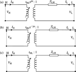
Figure 4.8 PPS and NPS equivalent circuits of Figure 4.4(b) for an off-nominal ratio two-winding three-phase transformer: (a) PPS equivalent circuit, (b) NPS equivalent circuit and (c) PPS and NPS equivalent circuit ignoring phase shift

Figure 4.9 PPS and NPS equivalent circuits of Figure 4.4(c) for an off-nominal ratio two-winding three-phase transformer: (a) PPS equivalent circuit, (b) NPS equivalent circuit and (c) PPS and NPS equivalent circuit ignoring phase shift
ZPS equivalent circuits
The ZPS equivalent circuit of a two-winding transformer is primarily dependent on the method of connection of the primary and secondary windings because the ZPS currents in each phase are equal in magnitude and are in phase. Also, the ZPS equivalent circuit and currents are affected by the winding earthing arrangements. In addition, a practical factor that can influence the magnitude of the ZPS impedances and make them appreciably different from the PPS impedances is the type of construction of the transformer magnetic circuit. The effect of transformer core construction will be dealt with later in this section, but we will now focus on the effect of the winding connection and any neutral earthing that may be present.
Before considering three-phase two-winding transformers of various winding connections, we will restate a basic understanding regarding ZPS currents in simple star-connected or delta-connected three sets of impedances. For ZPS currents to flow in a star-connected set of impedances, the neutral point of the star should be earthed either directly or indirectly, e.g. through an impedance. The ZPS current that flows to earth through this path is the sum of the ZPS currents in the three phases of the star impedances or three times the phase R ZPS current. For a delta-connected three-phase set of impedances, no ZPS currents will flow in the output terminals and hence inside the delta connection. However, ZPS currents can circulate inside the delta by mutual coupling but no ZPS current can emerge out into the output terminals of the delta. Figure 4.10(a) shows the impedance connections and ZPS current flows for the above three cases and Figure 4.10(b) shows the three-phase circuits and their corresponding ZPS equivalent circuits. It should be noted that because the voltage drop across the earthing impedance ZE is 3IZZE, the effective earthing impedance appearing in the ZPS equivalent circuit is 3ZE. The reader should easily demonstrate this.

Figure 4.10 ZPS equivalent circuits for three-phase impedances connected in star or delta: (a) three-phase star- and delta-connected impedances and (b) ZPS equivalent circuits
We will now derive approximate ZPS equivalent circuits for two-winding transformers of various winding connection arrangements. We emphasise that these are approximate because for now we ignore the effect of transformer core or magnetic circuit construction on the magnetising impedance. This is an important practical aspect that should not be ignored in practical short-circuit analysis. This is discussed in detail in Section 4.2.8.
The basic and fundamental principle that underpins the derivation of the approximate ZPS equivalent circuits is based on Equation (4.1b). This states that there is always a magnetic circuit MMF or ampere-turn balance for the transformer primary and secondary windings. That is, no current can flow in one winding unless a corresponding current, allowing for the winding turns ratio, flows in the other winding. In deriving the ZPS equivalent circuits of two-winding transformers of various winding connections, the winding terminal is connected to the external circuit if ZPS current can flow into and out of the winding. If ZPS current can circulate inside the winding without flowing in the external circuit, the winding terminal is connected directly to the reference zero voltage node. Figure 4.11 shows ZPS equivalent circuits for an off-nominal ratio transformer that correspond to Figures 4.8(c) and 4.9(c). These take account of any HV and LV winding connection arrangements, and any neutral impedance earthing that may be used.
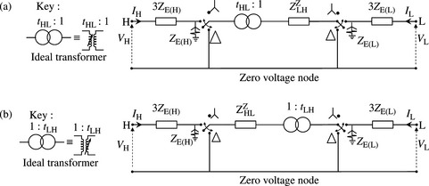
Figure 4.11 Generic ZPS equivalent circuits for two-winding transformers: (a) generic ZPS equivalent circuit of Figure 8.4(a) and (b) Generic ZPS equivalent circuit of Figure 4.9(c)
By making use of Figure 11.4(a) and (b), and noting that an arrow on a winding signifies the presence of a tap-changer on this winding, Figure 4.12 can be derived. This shows approximate ZPS equivalent circuits for the most common three-phase two-winding transformers used in power systems. It should be noted that ZE is in per unit on the voltage base of the winding to which it is connected.
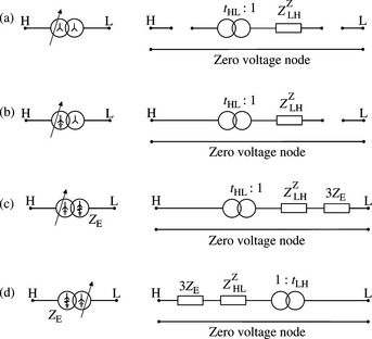

Figure 4.12 Approximate ZPS equivalent circuits for common three-phase two-winding transformers: (a) star-star with isolated neutrals; (b) star with solidly earthed neutral – star isolated neutral; (c) star solidly earthed – star neutral earthing impedance; (d) star neutral earthing impedance – star solidly earthed neutral; (e) star isolated neutral – delta; (f) delta-delta; (g) star neutral earthing impedance – delta and (h) delta-star neutral earthing impedance
Returning to the example shown in Figure 4.5, and assuming the transformer is a three-phase two-winding star (HV winding)-delta (LV winding) transformer, the ZPS equivalent circuits that correspond to each tap ratio condition are shown in Figure 4.13. The reader should find it instructive to obtain the three equivalent circuits shown in Figure 4.13 from the corresponding equivalent π circuits shown in Figure 4.7 by applying a short-circuit at end L and calculating the equivalent impedance seen from the H side.

The elements of the admittance matrix of Equation (4.17a), for the transformer winding connections and their equivalent circuits shown in Figure 4.12, can be easily derived using the following equations:
The results are shown in Table 4.1. The reader is encouraged to derive these results.
Table 4.1 Elements of ZPS admittance matrix of two-winding three-phase transformers
| Figure | Two-winding three-phase transformer winding connections | Elements of ZPS admittance matrix of Equation (4.19b) |
|---|---|---|
| 4.12(a) |
|
Y11 =Y12 =Y21 =Y22 = 0 |
| 4.12(b) |
|
Y11 =Y12 =Y21 =Y22 =0 |
| 4.12(c) |
|
 |
| 4.12(d) |
|
 |
| 4.12(e) |
|
Y11 =Y12 =Y21 =Y22 =0 |
| 4.12(f) |
|
Y11 =Y12 =Y21 =Y22 =0 |
| 4.12(g) |
|
 |
| 4.12(h) |
|
 |
Effect of winding connection phase shifts on sequence voltages and currents
The effect of three-phase transformer phase shifts on the sequence currents and voltages will now be considered. The presence of a phase shift between the transformer primary and secondary voltages, and currents, depends on the transformer primary and secondary winding connections. For transformers with a star-star or a delta-delta winding connections, the primary and secondary currents, and voltages, in each of the three phases are either in phase or out of phase, i.e. the windings are connected so that the phase shifts are either 0° or ± 180°. The former case is illustrated in Figure 14.4(a) and (b). British and IEC practices use ‘vector group reference’ number and symbol. In the symbol Yd1, the capital and small letters Y and d indicate HV winding star and LV winding delta connections, respectively, and the digit 1 indicates a phase shift of −30° using a 12 × 30° clock reference. For example, 0° indicates 12 o’clock, 180° indicates 6 o’clock, −30° indicates 1 o’clock and +30° indicates 11 o’clock.
In Figure 4.14, the 0° phase shift is achieved by ensuring that the parallel windings, i.e. same phase windings, are linked by the same magnetic flux. Figure 4.14 also shows that the absence of phase shifts in the phase currents and voltages also translates into the PPS, and NPS, currents and voltages. Consequently, the presence of such transformers in the three-phase network requires no special treatment in the formed PPS and NPS networks under balanced or unbalanced conditions. It should be noted that for the delta winding, although a physical neutral point does not exist, a voltage from each phase terminal to neutral does still exist because the network to which the delta winding is connected would in practice contain a neutral point.
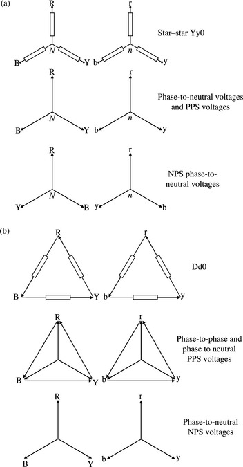
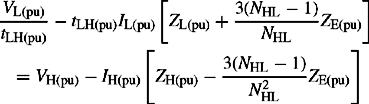
In the case of transformers with windings connected in star-delta (or delta-star), voltages and currents on the star winding side will be phase shifted by a ± 30° angle with respect to those on the delta side (or vice versa depending on the chosen reference). According to British practice, Yd11 results in the PPS phase-to-neutral voltages on the star side lagging by 30° the corresponding ones on the delta side. Also, Yd1 results in the PPS phase-to-neutral voltages on the star side leading by 30° the corresponding ones on the delta side. The example vector diagrams shown in Figure 4.15 for Yd1 and Yd1 1 illustrate this effect.

For RB Y/rby NPS phase sequence or rotation, Figure 4.15 also shows the effect of the Yd1 and Yd11 on the NPS voltage phase shifts and show that these are now reversed. These phase shifts also apply to the PPS and NPS currents in these windings because the phase angles of the currents with respect to their associated voltages are determined by the balanced load impedances only. In summary, where the PPS voltages and currents are shifted by +30°, the corresponding NPS voltages and currents are shifted by −30° and vice versa depending on the specified connection and phase shift, i.e. Yd1 or Yd11. Mathematically, this is derived for the Yd1 transformer shown in Figure 4.15 where n is the turns ratio as follows. The red phase current in amps flowing out of the d winding r phase is equal to Ir = n(IR – IB). Using Equation (2.9a) from Chapter 2 for phase currents and noting that ![]() because the in-phase ZPS currents cannot exit the d winding, we can write
because the in-phase ZPS currents cannot exit the d winding, we can write
or
where
or
or in per unit, where ![]()
Similarly, from Figure 4.15, the phase-to-neutral voltage in volts on the star winding R phase is
and using Equation (2.9b) for phase r and y voltages, we have
or
where
or
or in per unit, where ![]()
The reader is encouraged to derive the equations for the Yd11 transformer.
The American standard for designating winding terminals on star–delta transformers requires that the PPS (NPS) phase-to-neutral voltages on the high voltage winding to lead (lag) the corresponding PPS (NPS) phase-to-neutral voltages on the low voltage winding. This is so regardless of whether the star or the delta winding is on the high voltage side. In terms of sequence analysis, this means that when stepping up from the low voltage to the high voltage side of a star–delta or delta–star transformer, the PPS voltages and currents should be advanced by 30° whereas the NPS voltages and currents should be retarded by 30°. It is interesting to note the following observation on the British and American standards. In American practice, when the star winding in a star–delta transformer is the high voltage winding, this would correspond, in terms of phase shifts, to the Yd1 in British practice. However, when, in American practice, the delta winding in a star–delta transformer is the high voltage winding, this would correspond, in terms of phase shifts, to the Yd11 in British practice.
In terms of fault analysis in power system networks using the PPS and NPS networks, it is common practice to initially ‘ignore’ the phase shifts introduced by all star–delta transformers by assuming them as equivalent star–star transformers and to calculate the sequence voltages and currents on this basis. Then, having noted the locations in the network of such star–delta transformers, the appropriate phase shifts can be easily applied using the above equations as appropriate for the specified Yd transformer.
4.2.4 Three-phase three-winding transformers
Three-phase three-winding transformers are widely used in power systems. When the VA rating of the third winding is appreciably lower than the primary or secondary winding ratings, the third winding is called a tertiary winding. These windings are usually used for the connection of reactive compensation plant such as shunt rectors, shunt capacitors, static variable compensators or synchronous compensators or synchronous condensers. Tertiary windings may also be used to supply auxiliary load in substations and to generators. Delta-connected tertiary windings may also be used (and left unloaded) in order to provide a low impedance path to ZPS triplen harmonic currents. The B–H curve of the transformer magnetic circuit is non-linear and, under normal conditions, transformers do operate on the non-linear knee part of the curve. Thus, for a sinusoidal primary voltage, the magnetising current will be non-linear and will contain harmonic components which are mainly third harmonics. Since in three-phase systems, the third-order harmonic currents in each phase are in phase, they can be considered as ZPS currents of three times the fundamental frequency. Consequently, as for the ZPS fundamental frequency currents, the tertiary winding allows the circulation of third-order harmonic currents. Other benefits of Delta-connected tertiary windings is an improvement, i.e. a reduction in the unbalance of three-phase voltages.
Sometimes, for economic benefits, a third winding is usually provided to form a transformer with double-secondary windings. These transformers tend to be used to supply high density load in cities and this also provide additional benefits of fewer HV switchgear and also limiting LV system short-circuit currents where the two secondary LV terminals are not connected to the same busbar. Other uses are for the connection of two generators to a power network or for the connection of networks operating at different voltage levels.
Winding connections
There are several winding connections for three-phase three-winding transformers which may be used in power systems. Some examples are YNdd, Ydd, YNynyn, YNynd, YNyd and Yyd.
PPS and NPS equivalent circuits
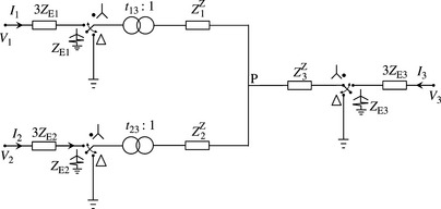
In a three-winding transformer, the three windings are generally mutually coupled although the degree of coupling between the two LV windings of a double secondary transformer can be chosen by design so that the LV windings are either closely or loosely coupled. Figure 4.16(a) shows a single-phase representation of a three-winding three-phase transformer ignoring, for now, the shunt exciting impedance.

Figure 4.16 Equivalent circuits for three-winding three-phase transformers: (a) single-phase representation in actual physical units; (b) PPS and NPS equivalent circuit with three off-nominal turns ratios and (c) PPS and NPS equivalent circuit with two off-nominal turns ratios
From Figure 4.16(a), the following equations in actual physical units can be written
Neglecting the no-load current, I0 = 0, and dividing Equation (4.20d) by N3, we obtain
Also
Using Equations (4.21b), (4.21c) and (4.20c), Equations (4.20a) and (4.20b) become
In most power system steady state analysis, we are more interested in deriving the three-winding transformer equivalent circuit in pu rather than in actual physical units. The following base and pu quantities are defined
Using Equations (4.23) and (4.24), Equations (4.22a) and (4.22b) become
 (4.25a)
 (4.25b)
Equations (4.25a) and (4.25b) can be rewritten as follows:
where, the following pu tap ratios are defined
 (4.27a)
 (4.27b)
 (4.27c)
Now, as in the case of two-winding transformers, we define
Substituting Equation (4.28) into Equation (4.26), we obtain
Using Equations (4.24c) and (4.27) in Equation (4.21a), we obtain
Equations (4.29) are represented by the equivalent circuit shown in Figure 4.16(b) where we have replaced the three-winding transformer with three two-winding transformers connected as three branches in a star configuration. Each branch corresponds to a winding and has its own general off-nominal tap ratio to represent a nominal, fixed off-nominal ratio or an on-load tap-changer, as required. The impedance of the magnetising branch Y0 can be inserted at the fictitious point P in the star equivalent circuit.
For improved applications in practice, Figure 4.16(b) can be further simplified to include only two off-nominal tap ratios instead of three as follows. Let
and
Substituting Equations (4.30) and (4.31) into Equation (4.26), we obtain
also, from Equation (4.29c), we have
Equations (4.32) are represented by the equivalent circuit shown in Figure 4.16(c) where, again, the three-winding transformer is replaced by three two-winding transformers connected as three branches in a star configuration. However, branch 3 now has an effective tap ratio of unity, t33(pu) = t3(pu)/t3(pu) = 1 as implied from Equations (4.30a) and (4.30b), although t3(pu) itself does not necessarily have to be equal to unity. The tap ratios included in the remaining two branches include the effect of branch 3 off-nominal tap ratio. This model would need to be used with care since, for example, the presence of a variable tap on one winding, say winding 3, must result in a coordinated and consistent change in the turns ratios between windings 1 and 3, and between windings 2 and 3.
Figure 4.16(b) or (c) represent the three-winding transformer PPS and NPS equivalent circuit if we ignore the windings phase shift. Otherwise, the only difference between the PPS and NPS equivalent circuits would be introduced by the windings phase shift. This was described in Section 4.2.3 and shown to result in a complex transformation ratio instead of a real one. In practice, the impedances of the three-winding transformer required in the equivalent circuit of Figure 4.16 are calculated from short-circuit test data supplied by the manufacturer. This will be covered in detail in Section 4.2.9.
The PPS/NPS star equivalent circuit of the three-winding transformer shown in Figure 4.16(b) can be converted into a delta equivalent circuit. We encourage the reader to do so.
As before, we will convert Figure 4.16(c) into π equivalents suitable for digital computer computation. We obviously obtain three π equivalents, one for each transformer branch as shown in Figure 4.17. It should be remembered that the π equivalents were derived with the convention that the currents are injected into them at both ends. Therefore, the currents flowing into the point P from the three branches would need to be reversed in sign.

ZPS equivalent circuits
The approximate ZPS equivalent circuits of three-winding transformers using various windings arrangements will be derived with the aid of a generic ZPS equivalent circuit as already presented in the case of two-winding transformers. Remembering that in Figure 4.16(c), we have converted the three-winding transformer into three two-winding transformers connected in star. Therefore, the generic ZPS equivalent circuit, ignoring the shunt exciting branch for now is shown in Figure 4.18 and is based on the following assumptions:
(a) The secondary of each two-winding transformer is assumed to be star connected with solidly earthed neutral, i.e. directly connected to point P.
(b) The primary of each two-winding transformer is assumed to have the same winding connection as one of the windings of the three-winding transformer.
The equivalent ZPS circuits for three-winding transformers having YNdd, Ydd, YNyd, YNynd, YNynyn and Yyd winding arrangements are shown in Figure 4.19.
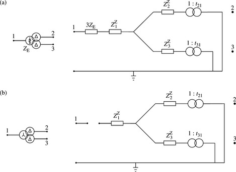
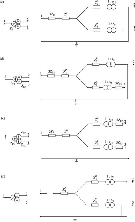
Figure 4.19 ZPS equivalent circuits of three-phase three-winding transformer: (a) star neutral earthing impedance – delta-delta; (b) star isolated neutral – delta-delta; (c) star neutral earthing impedance – delta-star isolated neutral; (d) star neutral earthing impedance – delta-star neutral earthing impedance; (e) all windings are star neutral earthing impedances and (f) star isolated neutral – star isolated neutral – delta
The elements of the admittance matrix of Equation (4.17a) can be derived for each equivalent ZPS circuit shown in Figure 4.19. This is similar to the derivation steps that resulted in Table 4.1. We will leave this exercise for the motivated reader!
4.2.5 Three-phase autotransformers with and without tertiary windings
The autotransformer consists of a single continuous winding part of which is shared by the high and low voltage circuits. This is called the ‘common’ winding and is connected between the low voltage terminals. The rest of the total winding is called the ‘series’ winding and is the remaining part of the high voltage circuits. The combination of the series-common windings’ produces the high voltage terminals. Figure 4.20 shows a three-phase representation of a star-star autotransformer with a delta tertiary winding. In the UK, autotransformers interconnect the 400 and 275 kV networks, the 400/275 and 132 kV networks, whereas in North America, they interconnect the 345 kV and 138 kV networks, the 500 kV and 230 kV networks, etc.
Figure 4.20 Star–star autotransformer with a delta tertiary winding: (a) three-phase representation and (b) single-phase representation
Winding connections
Three-phase autotransformers are most often star–star connected as depicted in Figure 4.20(a). The common neutral point of the star–star connection require the two networks they interconnect to have the same earthing arrangement, e.g. solid earthing in the UK although impedance earthing may infrequently be used. Most autotransformers have a low MVA rating tertiary winding connected in delta.
PPS and NPS equivalent circuits
Autotransformers that interconnect extra high voltage transmission systems are not generally equipped with tap-changers due to high costs. However, those that interconnect the transmission and subtransmission or distribution networks are usually equipped with on-load tap-changers in order to control or improve the quality of their LV output voltage under heavy or light load system conditions. Although some tap-changers are connected on the HV winding, most tend to be connected on the LV winding. Most of these are connected at the LV winding line-end and only a few are connected at the winding neutral-end.
A single-phase representation of the general case of an autotransformer with a tertiary winding is shown in Figure 4.20(b). Using S, C and T to denote the series, common and tertiary windings, we can write in actual physical units
Neglecting the no-load current, the MMF balance is expressed as
or
where
Using Equations (4.34b), (4.34c) and (4.33a), Equations (4.33b) and (4.33c) can be written as
 (4.35b)
Equation (4.35) can be represented by the star equivalent circuit shown in Figure 4.21(a) containing two ideal transformers as for a three-winding transformer.

Figure 4.21 PPS/NPS equivalent circuit of an autotransformer with a tertiary winding: (a) equivalent circuit in actual physical units; (b) as (a) above but with L and T branch impedances referred to H voltage base; (c) as (b) above but an autotransformer without a tertiary winding and (d) as (b) above but all quantities are in pu
The measurement of the autotransformer PPS and ZPS impedances using short-circuit tests between two winding terminals is dealt with later in this section. However, it is instructive to use Equation (4.35) to demonstrate the results that can be obtained from such tests. Using Equations (4.34a) and (4.35), the PPS impedance measured from the H terminals with the L terminals short-circuited and T terminals open-circuited is
Also, the impedance measured from the H terminals with the T terminals short-circuited and L terminals open-circuited is
Similarly, the impedance measured from the L terminals with the T terminals short-circuited and H terminals open-circuited is
To calculate the impedance of each branch of the T equivalent circuit in ohms with all impedances referred to the H side voltage base, let us define the measured impedances as follows:
where the prime indicates quantities referred to the H side.
Solving Equations (4.36d), (4.36e) and (4.36f) for each branch impedance, we obtain
Now, substituting Equations (4.36a), (4.36b) and (4.36c) into Equations (4.37a), (4.37b) and (4.37c), we obtain
Figure 4.21(b) shows the autotransformer PPS T equivalent circuit with all impedances in ohms referred to the H terminals voltage base. In the absence of a tertiary winding, Figure 4.21c shows the equivalent circuit of the autotransformer. Using Equations (4.38) in Equations (4.35), we obtain
 (4.39a)
 (4.39b)
Now, we will convert Equations (4.39) from actual units to pu values. To do so, we define the following pu quantities
Using Equations (4.40) in Equations (4.39a) and (4.39b), we obtain
 (4.41a)
 (4.41b)
Equations (4.41a) and (4.41b) can be rewritten as
where the following pu tap ratios are defined
 (4.43a)
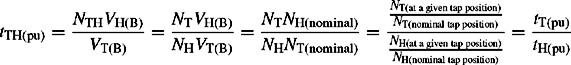 (4.43b)
Equations (4.42) are represented by the pu equivalent circuit shown in Figure 4.21(d) which represents the autotransformer PPS/NPS equivalent circuit ignoring the delta tertiary phase shift. The autotransformer is clearly represented as three two-winding transformers that are star or T connected. Two of these transformers have off-nominal tap ratios that can represent any off-nominal tap ratios on any winding or a combination of tap-ratios. In some cases, the two variable ratios must be consistent and coordinated where an active tap-changer on only one winding can in effect change the effective turns ratio on another. For example, for a 400 kV/132 kV/13 kV autotransformer having a tap-changer acting on the neutral end of the common winding, the variation of tLH(pu) caused by HV to LV turns ratio changes will also cause corresponding changes in the HV to TV turns ratio and hence in tTH(pu). Therefore, tTH(pu) is a function of tLH(pu) which varies as a result of controlling the LV (132 kV) terminal voltage to a specified target value around a deadband.
Where the autotransformer does not have a tertiary winding or where the tertiary winding is unloaded, the T terminal in Figure 4.21(d) would be unconnected to the power system network and its branch impedance has no effect on the network currents and voltages. Thus, this branch can be disregarded and the effective autotransformer impedance would then be the sum of the H and L branch impedances given by ZHL(pu) = ZH(pu) + ZL(pu). In this case, the PPS/NPS equivalent circuit of an autotransformer is similar to that already derived for a two-winding transformer and shown in Figures 4.8(c) or 4.9(c). These can be used to represent an autotransformer with ‘series’ winding tap-changer or ‘common’ winding tap-changer, respectively. The latter represents British practice irrespective of whether the tap-changer is connected to the line-end or neutral-end of the ‘common’ winding.
The impedances of the autotransformer required in the equivalent circuit of Figure 4.21(d) are calculated from short-circuit test data supplied by the manufacturer. This is covered in detail in Section 4.2.9.
ZPS equivalent circuits
In addition to the primary, secondary and, where present, tertiary winding connections, the presence of an impedance in the neutral point of the star-connected ‘common’ winding must be taken into account in deriving the autotransformers ZPS equivalent circuit. We will ignore, as before, the shunt exciting impedance, and consider the general case of a star–star autotransformer with a tertiary winding with the common star neutral point earthed through an impedance ZE. The ZPS equivalent circuit, taking into account the presence of ZE in the neutral, can be derived in a similar way to the PPS/NPS circuit. However, we will leave this as a minor challenge for the interested reader but we have drawn Figure 4.22 to help the reader in such derivation.

For us, it suffices to say that in Equations (4.35a) and (4.35b), ZC should be replaced by ZC + 3ZE. Therefore, the ZPS equations are given by
 (4.44b)
Similar to the derivation of the PPS impedances, the measured ZPS impedances between two terminals and the corresponding T equivalent branch impedances are
Substituting Equations (4.45d), (4.45e) and (4.45f) into Equations (4.44a) and (4.44b), we obtain
 (4.46a)
 (4.46b)
To convert Equations (4.46) to pu, we will use the base quantities defined in Equations (4.40) and define ZE(pu) = ZE/ZL(B), i.e. we choose to use the L terminal as the base voltage for converting ZE to pu. It should be noted that the choice of the voltage base for ZE is arbitrary. Therefore, Equations (4.46) become
 (4.46c)
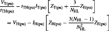 (4.46d)
where VT(pu) = 0. Equations (4.46c) and (4.46d) are represented by the ZPS T equivalent circuit of Figure 4.23 for a star-star autotransformer with a delta tertiary winding and with the common neutral point earthed through an impedance ZE. It is informative to observe how the neutral earthing impedance appears in the three branches connected to the H, L and T terminals
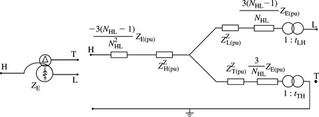
Figure 4.23 ZPS equivalent circuit of a star–star autotransformer with a neutral earthing impedance and a delta tertiary winding
where ZE(pu) is in pu on L terminal voltage base.
In the absence of a tertiary winding, the equivalent ZPS circuit cannot be obtained from Figure 4.23 by removing the branch that corresponds to the tertiary winding. A shunt branch to the zero voltage node may indeed still be required depending on the transformer core construction. This is covered in detail in Section 4.2.8.
The case of a solidly earthed neutral is represented in Figure 4.23 by setting ZE = 0. However, the case of an isolated neutral, i.e. ZE → ∞ cannot be represented by Figure 4.23 because the branch impedances of the equivalent circuit become infinite. This indicates no apparent paths for ZPS currents between the windings although a physical circuit does exist. A mathematical solution is to convert the star circuit of Figure 4.23 to delta or π and then setting ZE → ∞. However, we prefer the physical engineering approach to derive the equivalent ZPS circuit of such a transformer. Therefore, using the actual circuit of an unearthed autotransformer with a delta tertiary winding, shown in Figure 4.24(a), we can write

Figure 4.24 Derivation of ZPS equivalent circuit of an autotransformer with an isolated neutral and a delta tertiary winding: (a) autotranformer with isolated neutral and a delta tertiary winding; (b) single-phase representation; (c) tertiary impedance referred to series winding base turns; (d) equivalent ZPS circuit and impedance in physical units; (e) equivalent ZPS circuit in pu and (f) π ZPS equivalent circuit of (c)
Using Equations (4.48b), (4.48c) and (4.48d) in Equation (4.48a), we obtain
 (4.48e)
The measured ZPS leakage impedance in ohms
The ZPS leakage impedance measured from the H side or L side is the leakage impedance between the series and tertiary winding that is the sum of the series winding leakage impedance and the tertiary winding leakage impedance referred to the series side base turns. Figure 4.24(b) shows a single-phase representation of the series and tertiary winding impedances and turns ratios. Figure 4.24(c) shows the tertiary winding impedance referred to the series winding side and Figure 4.24(d) represents the ZPS equivalent circuit and total ZPS equivalent impedance in actual physical units. The physical explanation for this result is as follows. The ZPS currents flow on the H side through the series windings only and, without transformation, flow out of the L side. This is possible because the delta tertiary winding circulates equal ampere-turns to balance that of the series winding but no ZPS currents flow in the common windings of the autotransformer.
To convert Equation (4.48e) to pu, we first calculate a pu value for ZS–T and note that this is the same whether referred to the series winding or tertiary winding because the base voltages in the windings are directly proportional to the number of turns in the windings. Using Equation (4.40), we have
Equation (4.49a) is represented by the pu equivalent ZPS circuit shown in Figure 4.24(e) from which the ZPS leakage impedance measured from the H side with L side short-circuited is given by
Similarly, the ZPS leakage impedance measured from the L side with H side short-circuited is given by
The delta or π equivalent circuit can be derived using Figure 4.6(c). The result is shown in Figure 4.24(f) using shunt impedances instead of admittances.
Another similar test may be made but with the delta tertiary open to obtain the shunt ZPS magnetising impedance which may be low enough to be included depending on the core construction. This is dealt with in detail in Section 4.2.8.
4.2.6 Three-phase earthing or zig-zag transformers
Three-phase earthing transformers are connected to unearthed networks in order to provide a neutral point for connection to earth. In the UK, this arises in delta–connected tertiary windings and 33 kV distribution networks supplied via star–delta transformers from 132 or 275 kV networks which are solidly earthed. The purpose of using these transformers is to provide a low ZPS impedance path to the flow of ZPS short-circuit fault currents under unbalanced earthed faults. Such an aim can be achieved by the use of:
(a) A star-delta transformer where the star winding terminals are connected to the network and the delta winding is left unconnected. The star neutral may be earthed through an impedance.
(b) An interconnected star or zig–zag transformer which may also have a secondary star auxiliary winding to provide a neutral and substation supplies. The zig-zag neutral may be earthed through an impedance.
(c) An interconnected star or zig-zag as (b) above but with a delta-connected auxiliary winding.
The star–delta transformer has already been covered. However, in this case, its PPS and NPS impedance is effectively the shunt exciting impedance which is very large and can be neglected. The ZPS impedance is the leakage impedance presented by the star-delta connection discussed previously. The interconnected star or zigzag transformer has each phase winding split into two halves and interconnected as shown in Figure 25.4(a) and (b). It should be obvious from the vector diagram, Figure 4.25(c) that this winding connection produces a phase shift of 30° as if the zig-zag winding had a delta-connected characteristic. Again, the PPS/NPS impedance presented by this transformer if PPS/NPS voltages are applied is the very large exciting impedance. However, under ZPS excitation, MMF balance or cancellation occurs between the winding halves wound on the same core due to equal and opposite currents flowing in each winding half. The ZPS impedance per phase is therefore the leakage impedance between the two winding’s halves. In practical installations, the impedance connected to the neutral is usually much greater than the transformer leakage impedance. The zig-zag transformer ZPS equivalent circuit is shown in Figure 4.25(d).
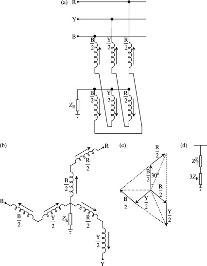
Figure 4.25 Interconnected-star or zig-zag transformer: (a) connection to a three-phase network, (b) winding connections, (c) vector diagram and (d) zps equivalent impedance
The zig-zag delta-connected transformer presents a similar ZPS equivalent circuit as the zig-zag transformer shown in Figure 4.25(d). If the delta winding is loaded, the transformer PPS/NPS equivalent circuit includes a 90° phase shift and is similar to that of a two-winding transformer with an impedance derived from the star equivalent of the three windings.
4.2.7 Single-phase traction transformers connected to three-phase systems
Single-phase traction transformers are used to provide electricity supply to trains overhead catenary systems and are connected on the HV side to two phases of the transmission or distribution network. In the UK, the secondary nominal voltage to earth of these single-phase transformers is 25 kV and their HV voltage may be 132, 275 or 400 kV. The 132 kV/25 kV are typically two-winding transformers whereas modern large units derive their supplies from 400 kV and tend to be three-winding transformers, e.g. 400 kV/26.25 kV-0–26.25 kV. Figure 4.26 illustrate such connections.

Figure 4.26 Single-phase traction transformer connected to a three-phase system: (a) two windings and (b) three windings
The model of two-winding single-phase traction transformers is the same as the single-phase model presented at the beginning of this chapter. Three-winding single-phase traction transformers can also be represented as a star equivalent of three leakage impedances. Under normal operating conditions, the traction load impedance referred to the primary side of the traction transformer appears in series with the transformer leakage impedance and is very large. However, under a short-circuit fault on the LV side of the traction transformer, the transformer winding leakage impedance appears directly on the HV side as an impedance connected between two phases. The reader should establish that this can be modelled as a phase-to-phase short-circuit fault through a fault impedance equal to the transformer leakage impedance.
4.2.8 Variation of transformer’s PPS leakage impedance with tap position
We have so far covered the modelling of the transformer with an off-nominal turns ratio that may be due to the use of a variable tap-changer or fixed off-nominal ratio. We have shown that, for some models, the leakage impedance, both PPS and ZPS, needs to be multiplied by the square of the off-nominal ratio. In addition, since the operation of the tap-changer involves the addition or cancellation of turns from a given winding, the variation of the number of turns causes variations in the leakage flux patterns and flux linkages.
The magnitude of the impedance variation and its direction in terms of whether it remains broadly unaffected, increases or decreases by the addition or removal of turns, depends on a number of factors. One factor is the tapped winding, e.g. whether in the case of a two-winding transformer, the HV or LV winding is the tapped winding. For an autotransformer, it is whether the series or common winding and in the latter case, whether the common winding is tapped at the line, i.e. output end or at the neutral-end of the winding. Other factors are the range of variation of the number of turns and the location of the taps, e.g. for a two-winding transformer, whether they are located in the body of the tapped winding itself, inside the LV winding or outside the HV winding. In summary, the addition of turns above nominal tap position or the removal of turns below nominal tap position may produce any of the following effects depending on specific transformer and tap-changer design factors:
(a) The leakage impedance remains fairly constant and unaffected.
(b) The leakage impedance may increase either side of nominal tap position.
(c) The leakage impedance may consistently decrease across the entire tap range as the number of turns is increased from minimum to maximum.
(d) The leakage impedance may consistently increase across the entire tap range as the number of turns is increased from minimum to maximum.
From a network analysis viewpoint, the leakage impedance variation across the tap range can be significant and this should be taken account of in the analysis. It is general practice in industry that the data of the impedance variation across the entire tap range is usually requested by transformer purchasers and supplied by manufacturers in short-circuit test certificates. The measurement of transformer impedances is covered in Section 4.2.10.
4.2.9 Practical aspects of ZPS impedances of transformers
In deriving the ZPS equivalent circuits for the various transformers we have presented so far, we only considered the primary effects of the winding connections and neutral earthing impedances in the case of star-connected windings. We have temporarily neglected the effect of the transformer core construction and hence the characteristics of the ZPS flux paths on the ZPS leakage impedances. Contrary to what is generally published in the literature, we recommend that the effect of transformer core construction on the magnitude of the ZPS leakage impedance is fully taken into account in setting up transformer ZPS equivalent circuits in network models for use in short-circuit analysis. We consider this as international best practice that in the author’s experience, can have a material effect during the assessment of short-circuit duties on circuit-breakers.
We will now consider this aspect in some detail and in order to aid our discussion, we will recall some of the basics of magnetic and electromagnetic circuit theory. The relative permeability of transformer iron or steel core is hundreds of times greater than that of air. The reluctance of the magnetic core is its ability to oppose the flow of flux and is inversely proportional to its permeability. The reluctance and flux of a magnetic circuit are analogous to the resistance and current in an electric circuit. Therefore, transformer iron or steel cores present low reluctance paths to the flow of flux in the core. Also, the core magnetising reactance is inversely proportional to its reluctance. Therefore, where the flux flows within the transformer core, the transformer magnetising reactance will have a very large value and will therefore not have a material effect on the transformer leakage impedance. However, where the flux is forced to flow out of the transformer core, e.g. into the air and complete its circuit through the tank and/or oil, then the effect of this external very high reluctance path is to significantly lower the magnetising reactance. This will substantially lower the leakage impedance of the transformer. It should be remembered that under PPS/NPS excitation, nearly all flux is confined to the iron or steel magnetic circuit, the magnetising current is very low and hence the PPS/NPS magnetising reactance is very large and has no practical effect on the PPS/NPS leakage impedance. We will now discuss the effect of various transformer core constructions on the ZPS impedance.
Three-phase transformers made up of three single-phase banks
Figure 4.27 illustrates two typical single-phase transformer cores. In both cases, the ZPS flux set up by ZPS voltage excitation can flow within the core in a similar way to PPS flux. Consequently, the ZPS magnetising impedance will be very large and the ZPS leakage impedance of such transformers will be substantially equal to the PPS leakage impedance.

Three-phase transformers of 5-limb core construction and shell-type construction
Figures 4.28 and 4.29 illustrate a 5-limb core-type and a shell-type three-phase transformers, respectively. The 5-limb design is widely used in the UK and Europe whereas the shell-type tends to be widely used in North America. In both designs, the ZPS flux set up by ZPS excitation can flow within the core and return in the outer limbs. Consequently, as in the case of three-banks of single-phase transformers, the ZPS magnetising impedance will be very large and the ZPS leakage impedance of such transformers will be substantially equal to the PPS leakage impedance. The measurement of sequence impedances will be dealt within the next section. However, it is appropriate to explain now that PPS leakage impedances are normally measured at nearly rated current whereas ZPS impedances are measured, where this is done, at quite low current values. Therefore, under actual earth fault conditions giving rise to sufficiently high ZPS voltages on nearby transformers with currents similar to those of the PPS tests, the transformer outer limbs may approach saturation and this lowers the ZPS magnetising impedance. Consequently, the measured ZPS impedance value may be somewhat higher than the actual value for core-type design and substantially higher for shell-type design that exhibits much more variable core saturation than the limb-type core. Nonetheless, these magnetising impedances remain relatively large in comparison with the leakage impedances and hence, it is usually assumed that the PPS and ZPS leakage impedances of such transformers are equal.


Three-phase transformers of 3-limb core construction
Figure 4.30 illustrates a three-phase transformer of 3-limb core-type construction which is extensively used in the UK and the rest of the world. Under ZPS voltage excitation, the ZPS flux must exit the core and its return path must be completed through the air with the dominant part being the tank then the oil and perhaps the core support framework. This ZPS flux will induce large ZPS currents through the central belt of the transformer tank and the overall effect of this very high reluctance path is to significantly lower the ZPS magnetising impedance. This ZPS magnetising impedance will be comparable to other plant values and may be 60–120% on rating for two and three-winding transformers and perhaps 150–250% for autotransformers. These figures can be compared with 5000–20 000% for the corresponding PPS values (these correspond to 2–0.5% no-load currents). Therefore, the effect of the tank for two-winding and three-winding transformers with star earthed neutral windings, and for autotransformers without tertiary windings, can be treated as if the transformer has a virtual magnetic delta-connected winding. We will provide practical examples of this in the next section.

Similar to 5-limb and shell-type transformers, ZPS leakage impedance measurements may be made at low current values and hence may give slightly higher impedances than the values inferred from PPS measurements made at rated current value. In addition, the effect of the tank in the 3-limb construction is non-linear with the reluctance increasing with increasing current that is the magnetising reactance decreasing with increasing current. Therefore, the actual ZPS leakage impedance of three-limb transformers may be slightly lower than the measured values.
4.2.10 Measurement of sequence impedances of three-phase transformers
Transformers are subjected to a variety of tests by their manufacturers to establish correct design parameters, quality and suitability for 30 or 40 years service life. The tests from which the transformer impedances are calculated are iron loss test, no-load current test, copper loss test, short-circuit PPS and sometimes ZPS impedance tests.
The iron loss and no-load current tests are carried out simultaneously. The rated voltage at rated frequency is applied to the LV winding, or tertiary winding where present, with the HV winding open-circuited. The shunt exciting impedance or admittance is calculated from the applied voltage and no-load current, and its resistive part is calculated from the iron loss. The magnetising reactance is then calculated from the resistance or conductance and impedance or admittance. The no-load current is obtained from ammeter readings in each phase and usually an average value is taken. The iron loss would be the same if measured from the HV side but the current would obviously be different as it will be in inverse proportion to the turns ratio. Also, the application of rated voltage to the LV or tertiary is more easily obtainable and the current magnitude would be larger and more conveniently read. The measured no-load loss is usually considered equal to the iron loss by ignoring the dielectric loss and the copper loss due to the small exciting current.
The copper loss and short-circuit impedance tests are carried out simultaneously. A low voltage is applied to the HV winding with the LV winding being short-circuited. The applied voltage is gradually increased until the HV current is equal to the full load or rated current. The applied voltage, measured current and measured load loss are read. As the current is at rated value, the short-circuit impedance voltage in pu is given by the applied voltage in pu of rated voltage of the HV winding. The load-loss would be the same if measured from the LV side. It is usual for transformers having normal impedance values to ignore the iron loss component of the load loss and the measured loss to be taken as the copper loss. The reason being is that the iron loss is negligible in comparison with the copper loss at the reduced short-circuit test voltage. Where high impedance transformers are specified, however, the iron loss at the short-circuit test voltage may not be negligible. In this case, the copper-loss can be found after reading the load-loss from the short-circuit test by removing the short-circuit (i.e. convert the test to an open-circuit test at the short-circuit applied voltage) reading the iron-loss and subtracting it from the load-loss. The resistance is calculated from the measured copper-loss and the reactance is calculated from the impedance voltage and the resistance.
The measurements made in volts and amps allow the calculation of the impedances in ohms but for general power system analysis, these need to be converted to per unit on some defined base. The equations presented below are straightforward to derive and we recommend that the reader does so.
From the open-circuit test, the exciting admittance Y(pu) = G(pu) – jBM(pu) is defined as follows:
where
and
The resistive (conductance) part of the exciting admittance is calculated as
where Fe[3-phase loss (MW)] is the iron loss.
The inductive part is calculated as
and
and
From the short-circuit test, the short-circuit leakage impedance Z(pu) = R(pu) + jX(pu) is defined as follows:
This is equal to the applied test voltage in pu which is why the term short-circuit impedance voltage is used by transformer manufacturers. This applies at nominal and off-nominal tap position.
The resistive part of the leakage impedance is calculated as
and the inductive part is calculated as

 (4.51c)
Whereas PPS impedance measurement tests for a number of tap positions such as minimum, maximum, nominal and mean have always been the norm, it is only recently becoming standard industry practice to similarly specify ZPS impedance tests. In the case of ZPS impedance measurements, the three-phase terminals of the winding from which the measurement is made are joined together and a single-phase voltage source is applied between this point and neutral. Voltage, current and copper loss may be measured; the ZPS resistance is calculated from the copper loss and input ZPS current. The ZPS impedance is calculated from the applied voltage and 1/3rd of the source current because the source ZPS current divides equally between the three phases. The basic principle of the PPS and ZPS leakage impedance tests is illustrated in Figure 4.31 for a star with neutral solidly earthed-delta two-winding transformer. It should be noted that, in the ZPS test, if the LV winding is delta connected, it must be closed but not necessarily short-circuited.
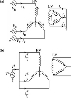
Figure 4.31 Illustration of PPS and ZPS test circuits on a star-delta two winding transformer: (a) PPS leakage impedance test, HV winding supplied, LV winding short circuited ![]() and (b) ZPS leakage impedance test, HV winding terminals joined and supplied, LV winding closed
and (b) ZPS leakage impedance test, HV winding terminals joined and supplied, LV winding closed![]()
PPS and ZPS impedance tests on two-winding transformers
The PPS impedance test is HV–LV//N, i.e. the HV winding is supplied with the LV winding phase terminals joined together, i.e. short-circuited and connected to neutral. The same test may be done for the ZPS impedance if the secondary winding is delta connected. However, for a star earthed-star earthed transformer, the ZPS equivalent circuit that correctly represents a 3-limb core transformer, is a star or T equivalent circuit since we represent the tank ZPS contribution as a magnetic delta tertiary winding. Therefore, at least three measurements are required. It is the author’s practice that four ZPS tests are specified to enable a better estimate of the impedance to neutral branch that represents the tank contribution. The ZPS tests are HV–N with LV phase terminals open-circuited, LV–N with HV phase terminals open-circuited, HV–LV//N with LV phase terminals short-circuited and LV–HV//N with HV phase terminals short-circuited.
PPS and ZPS impedance tests on three-winding transformers
In order to derive the star or T equivalent PPS circuit for such transformers from measurements, let the three windings be denoted as 1, 2 and 3, where:
Z12 is the PPS leakage impedance measured from winding 1 with winding 2 short-circuited and winding 3 open-circuited. P12 is the measured copper loss. Z13 is the PPS leakage impedance measured from winding 1 with winding 3 short-circuited and winding 2 open-circuited. P13 is the measured copper loss. Z23 is the PPS leakage impedance measured from winding 2 with winding 3 short-circuited and winding 1 open-circuited. P23 is the measured copper loss.
In three-winding transformers, at least one winding will have a different MVA rating but all the pu impedances must be expressed on the same MVA base. From the above tests, and with the impedances in ohms referred to the same voltage base, and copper losses in kW, we have
Solving Equations (4.52), we obtain
The winding copper loss measurements of Equation (4.52) can be used to calculate the corresponding winding resistances in ohms or in pu on a common MVA base. Then individual resistances are calculated from Equation (4.53). Alternatively, individual winding copper losses could be calculated using Equation (4.53) and used to calculate the corresponding individual winding resistances. When converted into pu, all impedances must be based on one common MVA base.
Regarding the ZPS impedances, the ZPS equivalent circuit that correctly represents a 3-limb core three-winding transformer even when all windings are star-connected, is a star or T equivalent circuit since we represent the tank ZPS contribution as a magnetic delta tertiary winding. Therefore, as in the case of the two-winding transformer, the ZPS tests are HV–N with LV phase terminals open-circuited, LV–N with HV phase terminals open-circuited, HV–LV//N with LV phase terminals short-circuited and LV–HV//N with HV phase terminals short-circuited.
Autotransformers
Generally, two cases are of most practical interest for autotransformers. The first is an autotransformer with a delta-connected tertiary winding and the second is without a tertiary winding. Without a tertiary winding, the PPS test is similar to that of a two-winding transformer described above. With a tertiary winding, the PPS tests are similar to those of a three-winding transformer. However, the ZPS equivalent circuit that correctly represents a 3-limb core autotransformer, with or without a tertiary winding, is a star or T equivalent circuit since we represent the tank ZPS contribution as a magnetic delta tertiary winding. Therefore, the ZPS tests are:
| With delta tertiary | Without tertiary | Comments |
|---|---|---|
| HV–Tertiary//N | HV–N | LV phase terminals open-circuited |
| LV–Tertiary//N | LV–N | HV phase terminals open-circuited |
| HV–LV//Tertiary//N | HV–LV//N | LV phase terminals short-circuited |
| LV–HV//Tertiary//N | LV–HV//N | HV phase terminals short-circuited |
4.2.11 Examples
Example 4.1
The rated and measured test data of a three-phase two-winding transformer are:
Rated data: 120 MVA, 275 kV star with neutral solidly earthed/66 kV delta, ± 15% HV tapping range
Test data: No-load current measured from LV terminals = 7 A
Iron loss = 103 kW, Full load copper loss = 574 kW
Short-circuit PPS impedance measured from HV side with LV side shorted =122.6 ω
Short-circuit ZPS impedance measured from HV side with LV side shorted =106.7 ω
Calculate the PPS and ZPS equivalent circuit parameters in pu on 100 MVA base


It is worth noting that the PPS X/R ratio is 16.195/0.398 = 40.7
This is 87% of the PPS impedance. In the absence of ZPS copper loss measurement, the ZPS X/R ratio may be assumed equal to the PPS X/R ratio of 40.7. Therefore,
and
If the PPS impedance were measured from the LV side, its ohmic value would be 122.6 × (66 kV/275 kV)2 = 7.06 ω and its pu value would also be equal to 16.2%.
Example 4.2
Consider a two-winding three-phase transformer with the following rated data: 45 MVA, 132 kV/33 kV star solidly earthed neutral – delta, HV winding tapped with –20% to +10% tap range. PPS impedance tests were carried out at all 19 tap positions with the HV terminals supplied by a three -phase voltage source and the LV winding short-circuited. The applied test voltages and full load currents on the HV side at minimum, nominal and maximum tap positions are:
| Tap position | Phase-phase voltage (V) | Current (A) |
|---|---|---|
| 1 (+10%) | 17 800 | 179 |
| 7 (nominal) | 15 560 | 197 |
| 19 (-20%) | 11 130 | 246 |
Calculate the measured impedance at each tap position both in ohms and in pu on MVA rating:
Rated tap voltage = 132 × 1.1 = 145.2 kV
Alternatively, impedance in pu on ![]()
Rated tap voltage = 132 × 1 = 132 kV, the impedance is 45.6 ω, or 11.8% on 45 MVA.
Rated tap voltage = 132 × 0.8 = 105.74 kV, the impedance is 26.1 ω or 10.6% on 45 MVA.
The reader should notice that the apparent small variation in impedance in % terms masks the significant change in the impedance when actual units, i.e. ohms are used. Also, the base impedance in each case is different because it is dependent on the rated tap voltage which is a function of the tap position.
Example 4.3
The rated and measured test data for a three-phase three-winding transformer are:
Primary HV winding 60.6 MVA, 132 kV star solidly earthed.
Secondary LV1 winding 30.3 MVA, 11.11 kV star solidly earthed.
Secondary LV2 winding 30.3 MVA, 11.11 kV star solidly earthed.
The construction is a 3-limb core. The short-circuit impedance and load loss measurement test data at nominal tap position is:

Derive the PPS and ZPS impedances and corresponding transformer equivalent circuits. Calculate the effective pu tap ratios at –10% turns HV winding tap position. The network base voltages are 132 and 11 kV. Use 60.6 MVA as a common base.

It is important to remember that the impedances in ω in the star or T equivalent of the three-winding transformer must all be referred to the same voltage base:

or
This should not alarm the reader because the T equivalent is a fictitious mathematical model!
The reactances of the T equivalent are given by XH = 27.97 ω or 9.7%;
XL1 = 162.86 ω or 56.6% and XL2 = 162.46 ω or 56.5%.
Designating terminals LV1 as 1, LV2 as 2 and HV as 3, the tap effective pu ratios at –10% HV winding turns are
The PPS and ZPS equivalent circuits are shown in Figure 4.32.
Example 4.4
A 3 limb core autotransformer has the following rated data: 275 kV/132 kV, 240 MVA, star–star solidly earthed neutral and a 60 MVA/13 kV tertiary winding. The HV to LV PPS impedance is 18.95% on 240 MVA rating. ZPS impedance tests were carried out with the delta winding closed and open to simulate the change in ZPS impedances if the transformer had no tertiary winding and to identify the effect of the core construction. The measured ZPS impedances at nominal tap position in both cases are:
| Measured impedance (ω/phase) | ||
|---|---|---|
| ZPS test | Delta closed | Delta open |
| 107.3 | 741.4 | |
| 14.3 | 200.5 | |
| 50.2 | 50.0 | |
| 6.8 | 13.5 | |
Derive general equations for the ZPS T equivalent circuit impedances and calculate the impedances for the above two cases in % on 100 MVA:

Using these equations, we obtain
| ZPS impedance (% on 100 MVA) | Delta closed | Delta open |
|---|---|---|
| 14.2 | 98 | |
| 8.2 | 115 | |
| 6.6 | 6.6 | |
| 3.9 | 7.8 |
The ZPS T equivalent circuit has three unknowns and therefore only three tests are required, e.g. the first three above. However, the fourth test, where available, can be used to improve the prediction of the shunt branch impedance. The four tests above are illustrated in Figure 4.33(a) from which we have the following:
Figure 4.33 ZPS leakage impedance tests on an autotransformer: (a) ZPS leakage impedance tests; (b) ZPS equivalent circuits

Substituting ![]() and
and![]() from the first two equations into the second two, we obtain
from the first two equations into the second two, we obtain
and a mean value is calculated as
The remaining H and L branch impedances are
The calculated ![]() and
and![]() for the closed and open delta tertiary are shown in Figure 4.33(b).
for the closed and open delta tertiary are shown in Figure 4.33(b).
Example 4.5
The autotransformer with a tertiary winding used in Example 4.3 has a neutral earthing reactor of 10 ω connected to its neutral. Calculate the earthing impedance values in % on 100 MVA base that would appear in each branch of the autotransformer ZPS T equivalent circuit.
The transformer turns ratio is 275/132 = 2.0834.
The % impedance value of the earthing reactor is
The earthing impedances appearing in the three branches of the ZPS T equivalent circuit are

4.3 Sequence modelling of QBs and PS transformers
4.3.1 Background
QBs and PS transformers are widely used in transmission and subtransmission power systems for controlling the magnitude and direction of active power flow mainly over parallel circuits in order to increase the power transfer capability across boundaries or interfaces. A single-core design is characterised by its simplicity and economy but suffers from disadvantages. These include the over voltages that may be imposed on the tap-changer due to its position in series with the main line as well as having a virtually zero impedance at nominal tap which may not be desirable if short-circuit current limitation is required. By far, the most commonly used design is the two-core design in either a single tank or two tanks where very large rating is required. Figure 4.34 shows a 400 kV QB rated at 2000 MVA and ± 11.3° phase shift. Figures 4.35(a) and 4.36(a) show QB and PS one-line diagrams, respectively. A simplified representation of the three-phase connections of typical large QBs and PSs are shown in Figures 4.35(b) and 4.36(b), respectively. The designs shown are those where both QB and PS consist of two transformers; a shunt transformer connected in star-star and a series transformer connected in delta-series star. The primary winding of the shunt transformer is called the exciting winding and the secondary is called the regulating winding. The primary delta of the series transformer is called the booster winding and the secondary is called the series winding because it is in series with the line.


Figure 4.35 QB transformer: (a) one-line diagram, (b) winding connections and (c) open-circuit vector diagram

Figure 4.36 PS transformer: (a) one-line diagram, (b) winding connections and (c) open-circuit vector diagram
The principles of operation of the QB and PS are similar. The control of the magnitude and direction of active power flow on the line is achieved by varying the phase angle shift across the series winding. The phase shift and its variation are obtained by an on-load (under-load) tap-changer acting on the regulating winding and deriving a variable voltage component across two phases, e.g. Y and B. This voltage is in quadrature with the input voltage. It is then injected by the booster transformer delta winding across the series winding third phase, e.g. phase R, as shown in Figures 4.35(c) and 4.36(c). One important difference to notice between a QB and a PS is that for a QB, the input voltage of the shunt transformer is derived from one side of the series transformer so that the output voltage is slightly higher than the input voltage. However, for a PS, the shunt transformer input voltage is derived from the mid-point on the series winding of the series transformer so that the magnitudes of the input and output voltages remain equal.
4.3.2 PPS, NPS and ZPS modelling of QBs and PSs
PPS equivalent circuit model
The derivation of QB and PS detailed equivalent circuits needs to take into account both the shunt and series transformers, their winding connections, tap-changer operation, complex turns ratio and leakage impedance variations with tap position. However, we will instead present a simplified treatment but one that is still sufficient for use in practice in PPS power flow, stability and short-circuit analysis. The analysis below is based on the vector diagrams of Figures 4.35(c) and 4.36(c). These allow us to represent the QB or PS as an ideal transformer with a complex turns ratio in series with an appropriate impedance. This ratio is in series with a single effective leakage impedance representing both the series and shunt transformers’ leakage impedances including the effect of the tap-changer on the shunt transformer’s impedance. This representation is shown in Figure 4.37.
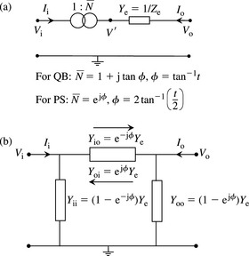
Figure 4.37 PPS equivalent circuits for a QB or a PS: (a) PPS equivalent circuit and (b) asymmetrical π equivalent circuit for a PS
For both a QB and a PS, let t = δ Vi(R)/Vi(R) be the magnitude of the injected quadrature voltage in pu of the input voltage. From the QB vector diagram shown in Figure 4.35(c), the phase R open-circuit output voltage phasor is given by
Let ![]() be defined as the complex turns ratio, at no load, thus,
be defined as the complex turns ratio, at no load, thus,
is the phase angle shift that has a maximum or rated value for practical QBs used in power networks of typically less than or equal to ± 15°. Similar equations apply for the Y and B phases.
Similarly, from the PS vector diagram shown in Figure 4.36(c), the phase R open-circuit output voltage is given by
where ViS(R) is the voltage at the mid-point of the series winding.
The complex turns ratio of the PS, at no load, is given by
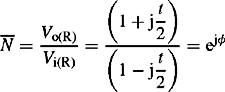 (4.55b)
where
is the phase angle shift that has a maximum or rated value for practical PSs used in power networks of typically less than or equal to ±60°.
Let Ye = 1/Ze where Ze is the effective QB or PS leakage impedance appearing in series with the line or the network where the device is connected. The QB and PS are both represented by the same PPS equivalent circuit shown in Figure 4.37. The PPS admittance matrix for this circuit can be easily derived as in the case of an off-nominal-ratio transformer but with an important difference now that the turns ratio is a complex number. From Figure 4.37, we can write
From these equations, the following admittance matrix is obtained
 (4.56a)
which, using Equations (4.54b) and (4.54c), can be written as
or, using Equation (4.55b), can be written as
The above two admittance matrices for a QB and a PS cannot be represented by a physical π equivalent circuit because the complex turns ratio has resulted in matrices that are non-symmetric, i.e. the off-diagonal transfer terms are not equal. However, recognising that an asymmetrical non-physical π equivalent circuit is simply a mathematical tool, such a circuit is shown in Figure 4.37(b) for a PS. A similar π equivalent for a QB can be derived and the reader is encouraged to derive this equivalent.
NPS equivalent circuit model
Since the QB and PS are static devices, the NPS impedance should be the same as the PPS impedance. However, we have shown that the PPS model includes a complex turns ratio which is a mathematical operation that introduces a phase angle shift in the output voltage (and current) with respect to the input voltage (and current). The mathematical derivation of the phase shift in the QB or PS NPS model requires a detailed representation of all windings of the shunt and series transformers, which, as outlined above, is not presented here. However, we will use vector diagrams to show that the phase shift in the NPS circuit is equal to that in the PPS circuit but reversed in sign. Figures 4.38(i) show the PPS open-circuit vector diagrams of a QB and a PS and the resultant phase angle shift φ in each case. Figures 4.38(ii) show the NPS vector diagrams of a QB and a PS and the resultant phase angle shift in each case.

Figure 4.38 PPS, NPS and ZPS vector diagrams for a QB and a PS: (a) QB vector diagram and (b) PS vector diagram
It is clear that with the reversed NPS phase rotation RBY, the injected series quadrature voltage vector is also reversed, for both QB and PS. Therefore, if the PPS phase angle shift is φ, then the NPS phase angle shift is –φ. Figure 4.39 shows the QB or PS NPS equivalent circuit model where the complex ratio is given by

Figure 4.39 NPS and ZPS equivalent circuits for a QB or a PS: (a) NPS equivalent circuit and (b) ZPS equivalent circuit
 (4.57a)
Using the PPS admittance matrices fora QB and a PS, the NPS admittance matrices are easily obtained by replacing φ with -φ in Equations (4.56b) and (4.56c).
ZPS equivalent circuit model
We have already stated that the basic principle of operation of the QB or PS is to inject a voltage across, say phase R, series transformer series winding that is in quadrature with the phase R input voltage. In the PPS and NPS circuits, this is achieved by deriving the injected voltage so as to be in phase or out of phase with the voltage difference between phases Y and B as shown in Figure 38.4(a) and (b), respectively. However, since the three ZPS voltages are in phase with each other, a quadrature voltage component cannot be produced. Therefore, the phase shift between the input and open-circuit output voltages (and currents) in the ZPS circuit is zero. Therefore, the complex turns ratio in the ZPS equivalent circuit for both a QB and a PS becomes unity.
The QB or PS practical ZPS equivalent circuit, however, is different from the PPS and NPS equivalent circuits. The ZPS equivalent circuit is dependent on the winding connections of the series and shunt transformers, their core construction and whether the shunt transformer has any delta-connected tertiary winding. In a similar way to a three-winding transformer, or a 3-limb core autotransformer with or without a tertiary winding, the general ZPS equivalent circuit of a QB or a PS is a star or T equivalent as shown in Figure 4.39(b). The shunt branch in this equivalent represents either the impedance of a tertiary winding or the stray air path ZPS flux through the tank/oil. In addition, in some QBs and PSs, both series and shunt transformers are in the same tank so that the ZPS flux can link both windings either directly or through the tank. In practice, the QB or PS ZPS impedances are derived from a series of manufacturer works-tests and this is described in the next section. The ZPS admittance matrix model of the QB or PS is given by
where
4.3.3 Measurement of QB and PS sequence impedances
Like transformers, QBs and PSs are subjected to a variety of works-tests by their manufacturers. As most QB and PS are three-phase two-transformer devices, tests are usually carried out on each transformer alone and on the combined units. No-load loss, load loss, PPS impedance and ZPS impedance tests are carried out on the combined units. The PPS impedance and load loss tests are carried out simultaneously with the output end of the series transformer supplied by three-phase voltage sources and the shunt transformer input terminals short-circuited. The ohmic value of the impedance is the applied voltage divided by the measured current. The pu value of the impedance must be expressed on the voltage base of the winding energised or supplied under the tests. Under such a test, the PPS impedance measured is the series combination of the leakage impedances of the series and shunt transformers. This can be easily visualised by referring back to the QB and PS winding connections shown in Figures 4.35 and 4.36. Therefore, this impedance is the QB or PS effective PPS impedance Ze that appears in series with the line as seen from the QB or PS series transformer output end.
The series transformer does not have a tap-changer so its leakage impedance, when measured from its output terminals, is constant. However, when measured from the same terminals, the shunt transformer leakage impedance varies with tap position as the tap-changer acts on the shunt transformer regulating winding. The variation of tap position varies the magnitude of the injected quadrature voltage and, the PPS/NPS leakage impedance will vary with the square of the injected quadrature voltage t. Therefore,
which can be expressed in terms of the phase angle shift as follows:
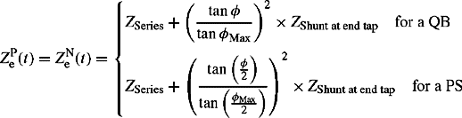 (4.59)
where φMax is the QB or PS rated or maximum phase shift design value, φ the actual phase shift in operation and ZShunt at end tap is the shunt transformer leakage impedance measured at end tap position that is at maximum quadrature voltage or maximum phase shift. It should be noted that Ze(φ = 0) is equal to ZSeries because the booster delta winding of the series transformer is effectively short-circuited by the tap-changer when a zero quadrature voltage is injected.
Like transformers, the ZPS leakage impedance tests are carried out applying a single-phase voltage source to three-phase input or output terminals joined together. Usually three or four such tests may be carried out to derive the star ZPS equivalent circuit. Some tests that may be carried out are described below where T represents a tertiary winding, where present in the shunt transformer, and N represents neutral. Reference is made to Figures 4.35 and 4.36 to see the designated QB and PS terminals.
| Terminals supplied | Designation | Comments |
|---|---|---|
| R1Y1B1 terminals joined together | Zol–T//N | R2Y2B2 terminals open-circuit, tertiary closed, where present |
| R2Y2B2 terminals joined together | Zo2–T//N | R1Y1B1 terminals open-circuit, tertiary closed, where present |
| R1Y1B1 terminals joined together | Zol–2//T//N | R2Y2B2 terminals short-circuited, tertiary closed, where present |
| R2Y2B2 terminals joined together | Zo2–1//T//N | R1Y1B1 terminals short-Circuited, tertiary closed, where present |
Example 4.6
A 400 kV 2000 MVA throughput QB has a rated quadrature injected voltage of ±0.2 pu of input voltage. The following PPS and ZPS impedance tests were carried out. In the PPS tests, the output, i.e. series transformer terminals R2Y2B2 are supplied and the input of the shunt transformer terminals R1Y1B1 are short-circuited.
| PPS Test | Phase-phase voltage (V) | Current (A) |
|---|---|---|
| Tapl | 56 800 | 2887 |
| Tap 20 (nominal) | 28 049 | 2886 |
| Tap 39 | 56 920 | 2888 |
| ZPS Test | Voltage (V) | Current (A) |
| Zo1–T//N | ||
| Tap 1 | 20 817 | 260.1 |
| Tap 20 (nominal) | 20 823 | 260.4 |
| Tap 39 | 20 818 | 260.4 |
| Zo2–T//N | ||
| Tap 1 | 21395 | 260.8 |
| Tap 20 (nominal) | 21360 | 260.4 |
| Tap 39 | 21377 | 260.5 |
| Zo2–1//T//N | ||
| Tap 1 | 506 | 260.0 |
| Tap 20 (nominal) | 507 | 260.7 |
| Tap 39 | 506 | 260.4 |
Calculate the open-circuit rated phase shift and output voltage of the QB for a 1 pu input voltage. Also, calculate the effective PPS impedance of the QB and the ZPS star equivalent impedances at nominal, minimum and maximum tap positions.
The open-circuit rated phase shift is tan−1(±0.2) = ±11.3°. The QB range of rated injected voltage or phase shift is from –0.2 pu corresponding to -11.3° phase shift to +0.2 pu corresponding to +11.3° phase shift. The open-circuit output voltage at rated phase shift is ![]() . The PPS impedance is calculated as follows:
. The PPS impedance is calculated as follows:
Alternatively, impedance in pu on ![]()
Impedance is 7.01% on 2000 MVA.
Impedance is 14.23% on 2000 MVA.
We note that the PPS impedance effectively doubles between nominal tap position (tap 20) and maximum/minimum tap positions (tap 39 and tap 1). The results of the calculated ZPS impedances are given as:

We note that the ZPS impedances of the equivalent star are effectively unaffected by variation of tap position. The impedances of the individual T branch equivalent circuit at nominal tap position in % on 2000 MVA and 400 kV are:
![]() where 1 corresponds to the shunt transformer’s input end R1Y1B1.
where 1 corresponds to the shunt transformer’s input end R1Y1B1.
![]() where 2 corresponds to the series transformer’s output end R2Y2B2.
where 2 corresponds to the series transformer’s output end R2Y2B2.
![]() where N corresponds to neutral or zero voltage reference in this case.
where N corresponds to neutral or zero voltage reference in this case.
Example 4.7
A 132 kV, 300 MVA throughput PS has a rated phase shift of ±30° and the shunt transformer unit includes a tertiary winding. The PPS impedance measured at nominal tap position is 2% on 100 MVA at 132 kV. The ZPS impedances of the PS are largely unaffected by variation of tap position and the ZPS impedance test data are as follows:

Calculate the ZPS star equivalent circuit impedances in % on 100 MVA.
Like autotransformers, we have four tests but only three unknowns so we will calculate two values of the shunt impedance in the star equivalent and obtain a mean value as follows:
and
and the mean value is ZN(mean)Z = 12.96 ω
The impedance values in % on 100 MVA are

4.4 Sequence modelling of series and shunt reactors and capacitors
4.4.1 Background
Series reactors are widely used in power systems for power flow control or as fault current limiters. The latter application will be covered in Chapter 9. Series reactors are generally used in electric distribution, subtransmission and transmission systems as well as power stations and industrial power systems. Air core reactors are usually used at nominal system voltages up to and including 36 kV, but iron-cored reactors are generally used at higher voltages. The former is usually coreless and magnetically or electromagnetically shielded and the latter are usually oil filled and gapped. Three-phase gapped iron core reactors look in appearance similar to a three-phase three-limb core transformer. However, reactors have only one winding on each limb. The function of the gaps in the core is to lower the flux density so that under high current conditions, the core barely enters into saturation and the reactor’s impedance remains substantially constant. In practice a decrease in the impedance from the rated current value by a few percent is typical. Magnetically shielded coreless reactors use shields to surround the windings in order to provide a return path for the winding flux. However, saturation and hence impedance reduction can still occur. In the electromagnetically shielded coreless reactor, the impedance remains virtually constant but with an increase in reactor cost.
Shunt reactors are widely used in power networks at various voltage levels for controlling and limiting transient and steady state voltages. Shunt reactors are cost-effective and robust reactive compensation devices used in absorbing surplus reactive power supply in cable systems where they may be switched in and out of service with the cable itself by the cable circuit-breakers. Many aspects of their design are similar to those of three-limb series reactors except that at higher voltages, many shunt reactors are star connected with their neutral point either solidly or impedance earthed.
Shunt capacitors are usually mechanically switched, i.e. by circuit-breakers and are very cost-effective reactive compensation devices that are extensively used in transmission and lower voltage power networks. They provide a source of reactive power supply and help to improve network voltage stability, voltage levels and power factors. Shunt capacitors can be star connected with the neutral isolated or solidly earthed, or delta connected, depending on the nominal system voltage.
Series capacitors are also widely used in transmission and distribution networks. In distribution, they are mainly used to improve the voltage profile of heavily loaded feeders. In transmission, they are mainly used to increase network power transfer capabilities by improving generator and network transient stability, damping of power oscillations, network voltage stability or load sharing on parallel circuits.
4.4.2 Modelling of series reactors
In a three-limb design of a three-phase series reactor, the winding around each limb represents one phase and the flux in any phase does not link that in the other two phases. Therefore, there is practically little or no mutual inductive coupling between the phases of the reactor. In addition, the phase windings are practically identical by design. A three-phase equivalent circuit is shown in Figure 4.40 where Z =R + jX is the leakage impedance per phase. The series phase voltage drop is given by
 (4.60a)
 (4.60b)
or in the sequence component reference frame expressed in terms of phase R,
 (4.60c)
Therefore, the PPS, NPS and ZPS admittances are all self-terms, as the phase admittances, and all are equal to 1/Z.
For some designs, the three-phase windings of the reactor are vertically stacked on top of each other as illustrated in Figure 4.41.

In such arrangement, the flux in one phase can link with the other phases and mutual inductive coupling between the three phases can therefore exist with the middle phase seeing more linked flux than the outer phases. This means that whilst the self-impedances are equal, the mutual impedance between the outer phases and that between the adjacent phases are not equal. Therefore, from Figure 4.41, we define the following:
Therefore, the series phase impedance matrix is written as
 (4.61a)
The series sequence impedance matrix can be easily calculated using ZPNZ = H−1ZRYBH, where H is the transformation matrix. Thus,
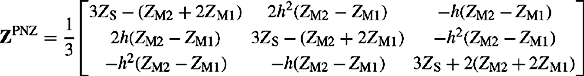 (4.61b)
This sequence impedance matrix is full and is not symmetric, i.e. it shows unequal intersequence mutual coupling, which as discussed in Chapter 2, eliminates the fundamental advantage of using the sequence component reference frame. However, in practice, for many vertical reactor designs, the vertical insulators between the phases are deliberately chosen to be sufficiently long so that the mutual coupling between the adjacent phases is quite small. In such cases, two practical options exist. The simplest, which is the one mostly used, is to ignore the small mutual coupling and set ZM1 = ZM2 = 0 so that the sequence impedance matrix reduces to
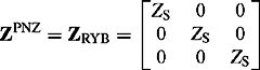 (4.61c)
The second option, where the mutual impedances are known, is to set them to a mean value ZM(mean) = (ZM1 + ZM2)/2. In this case, the series phase impedance matrix of Equation (4.16a) becomes
 (4.61d)
The corresponding series sequence impedance matrix is given by
 (4.61e)
The PPS and NPS impedances are equal to ZS –ZM(mean) and the ZPS impedance is equal to ZS + 2ZM(mean). The series sequence admittance matrix is given by
 (4.61f)
4.4.3 Modelling of shunt reactors and capacitors
In three-phase shunt reactors, there is practically negligible mutual coupling between the phases. Three-phase shunt reactors and capacitors depicted in Figure 4.42 are each representedas three identical shunt susceptances. The resistive part of the shunt reactor is normally neglected since, by design, these are required to have very high X/R ratios in the order of 100–200 to minimise active power losses. The internal series resistance of shunt capacitors is negligibly small. The phase and sequence admittance matrix of a shunt reactor or shunt capacitor is given by

Figure 4.42 Star-connected three-phase shunt reactors and capacitors: (a) three-phase shunt reactor and (b) three-phase shunt capacitor
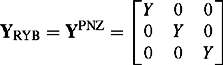 (4.62a)
where
and
The PPS, NPS and ZPS susceptances are equal. The magnitude of the susceptance is derived from the three-phase rated MVAr data of the reactor or capacitor as follows:
The pu susceptance is given by

or
For example, the susceptance of a 150 MVAr shunt reactor or capacitor in per cent on a 100 MVA base is equal to 150%.
Figure 4.43 shows two typical shunt capacitors used in 132 kV and 400 kV power systems.

4.4.4 Modelling of series capacitors
Types of series capacitor schemes
There are several three-phase series capacitor scheme designs in use in power systems, four of which are depicted in Figure 4.44.

General modelling aspects of series capacitors
The modelling of series capacitor schemes in power flow analysis is straightforward because the magnitude of current flowing through the capacitor would be within its appropriate rated design value. These rated values include not only the highest continuous current, but also the highest short-term overload value permitted and the highest permitted value under power oscillation conditions. The capacitors are therefore represented as three identical series reactances and the ohmic value of the reactance is known from the rated data. The resistive part of the series capacitor is negligibly small. Therefore, the sequence and phase admittance matrix of a three-phase series capacitor is given by
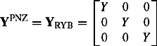 (4.63)
The PPS, NPS and ZPS admittances are equal.
However, for short-circuit analysis, the modelling of series capacitors is not straightforward and requires knowledge of the capacitor protection scheme and capacitor design ratings. It is worth noting that IEC 60909–0:2001 short-circuit analysis standard states that the effect of series capacitors can be neglected in the calculation of short-circuit currents if they are equipped with voltage-limiting devices in parallel acting if a short-circuit occurs. However, as we will see later, this approach is generally inappropriate for varistor protected series capacitors and could result in significant underestimates in the magnitude of short-circuit currents.
Modelling of series capacitors for short-circuit analysis
Old series capacitor schemes were protected by spark gaps against a short-circuit fault that can cause a large capacitor current to flow and a substantial increase in the voltage across the capacitor. The flashover across the spark gap bypasses the series capacitor and the bypass circuit-breaker is immediately closed to extinguish the gap.
In modern series capacitor installations, non-linear resistors are used and these are called metal (usually zinc) oxide varistors (MOVs) known as ZnO. MOVs are used to provide the overvoltage protection mainly against external short-circuit faults, i.e. external to the series capacitor and its line zone. For internal faults, within the series capacitor protected line zone, a forced triggered spark gap can operate typically within 1 ms to limit the energy absorption duty on the varistors. This is then followed by closure of the circuit-breaker to extinguish the gap and hence the capacitor is completely bypassed and removed from the circuit.
The modelling and analysis of varistor protected series capacitors under external or remote short-circuit fault conditions is quite complex. However, we will briefly and qualitatively describe the operation of the modern varistor protected capacitor schemes under external through-fault conditions that result in varistor operation only. As the instantaneous short-circuit current flowing through the capacitor increases, so will the voltage across the capacitor or varistor until this voltage reaches a preset threshold where the varistor starts conducting current in order to keep the voltage across the capacitor constant. This applies under both positive and negative polarity current conditions so that for the first part of each half cycle, the current flows through the capacitor only but for the other part of the half cycle, the current switches to the varistor. The behaviour of the varistor and series capacitor combination is repeated every half cycle during the fault period whenever the voltage across the capacitor/varistor exceeds the preset capacitor protection level. Using Figure 4.45(a), the behaviour of the series capacitor/varistor parallel combination under a through fault condition is analysed using an electromagnetic transient analysis program. The voltage across the capacitor/varistor and the currents through the capacitor and varistor are shown in Figure 4.45(b)–(d), respectively. The fault current is shown in Figure 4.45(e) curve (ii).

Figure 4.45 Behaviour of a series capacitor/varistor combination under external through-fault conditions: (a) generic circuit; (b) capacitor voltage; (c) capacitor current; (d) varistor current; and (e) fault current
Curve (i) of Figure 4.43(e) shows the fault current that would flow through the capacitor if there were no varistor to protect it. Clearly, the conduction of the MOV causes an effective reduction in the fault current magnitude. The extent of reduction is dependent on the electrical proximity of the fault location to the capacitor/varistor location. In addition, curve (iii) of Figure 4.45(e) shows the fault current if the capacitor is assumed to be permanently bypassed. This generic study illustrates that in general, both ignoring the presence of the varistor or assuming the capacitor is permanently bypassed during the fault period can result in a large error in the fault current magnitude. The former can result in an overestimate whereas the latter can result in an underestimate.
The modelling and analysis of short-circuit faults in large-scale power systems is based on the assumption that all power system plant are linear or can be approximated as piece-wise linear. The varistor is, however, a highly non-linear resistor that cannot be directly included in standard quasi-steady state short-circuit modelling and analysis simulations. Figure 4.46 shows a typical voltage/current characteristic of a varistor which presents an almost infinite resistance below the threshold conduction voltage then a very low resistance above it.
The impedance presented by the combined capacitor reactance and varistor resistance over a half cycle is dependent on the total current flowing through their parallel combination. The capacitor current or voltage protection threshold is known because the capacitor reactance is a known design parameter. Therefore, below this threshold, the equivalent impedance of the parallel capacitor/varistor combination is the capacitor reactance in parallel with a very high resistance or alternatively, a very low resistance (practically zero) in series with the capacitor reactance. When a current higher than the threshold flows through the capacitor, the varistor will conduct current for most of the half cycle so that the combination will appear as a low resistance in parallel with the capacitor reactance or, alternatively, a higher resistance than zero in series with a much reduced capacitor reactance. The higher the current is, the more resistive the equivalent impedance becomes reflecting the increased short-circuiting of the capacitor by the varistor. Therefore, the capacitor/varistor parallel combination can be approximated as a resistance and a capacitance in series with both being functions of the total current flowing through them. Figure 4.47(a) shows a three-phase representation of a series capacitor protected by a varistor. Figure 4.47(b) shows the corresponding equivalent circuit where the equivalent series impedance is a function of the total current flowing through the parallel capacitor/varistor combination.
Figure 4.47 Varistor-protected three-phase series capacitor and equivalent circuit: (a) three-phase representation and (b) equivalent circuit model
Denoting the capacitor current protective threshold as Ithr, the equivalent series impedance for each phase is given by
where XC is the capacitor reactance when all current flows through it, i.e. its nominal design value, I is the total current flowing through the capacitor/varistor parallel combination and Ithr is a known design threshold parameter. The mathematical functions that describe REq(I) and XEq(I) as functions of I when I ≥ Ithr can be calculated from the known design data or parameters of the series capacitor and varistor. Figure 4.48 illustrates typical equivalent impedance characteristics.
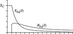
Figure 4.48 Typical equivalent impedance of a series capacitor/varistor combination under external through-fault conditions
The series phase admittance matrix of the three-phase series capacitor/varistor device is given by
 (4.65)
Prior to the short-circuit fault or when the current is less than Ithr, the equivalent phase admittances are balanced and equal. This will also be the case under balanced three-phase short-circuit faults. However, under unbalanced short-circuit faults, they are generally unequal depending on the fault type. Therefore, the sequence admittance matrix of Equation (4.65) is given by

where
 (4.66b)
Equation (4.66a) shows the presence of unequal intersequence mutual coupling which should be taken into account if significant errors are to be avoided.
Because fixed impedance short-circuit analysis techniques are linear, Equation (4.64) may be implemented in an iterative linear calculation process. The fault currents flowing in the network and the series capacitors are initially calculated without varistor action, the capacitor current is then used to calculate a new value for the series capacitor equivalent impedance using Equation (4.64). The new impedance is then used to calculate new fault currents in the network and the series capacitor. The final solution would be arrived at when there is a little change in the last two equivalent impedances or capacitor currents calculated.
In power system networks with modern varistor protected series capacitor installations, the operation of the varistor when the capacitor current exceeds Ithr cannot be ignored if very large and unacceptable errors (overestimates) in the calculated short-circuit currents in the network are to be avoided. Also, if these series capacitors are not included in the network model at all, i.e. assumed to be completely bypassed under short-circuit faults, as per IEC 60909, then this could result in significant underestimates in the magnitude of short-circuit currents.
4.5 Sequence modelling of static variable compensators
4.5.1 Background
Static variable compensators, with one typical arrangement shown in Figure 4.49(a), are shunt connected devices used in transmission, subtransmission, distribution and industrial power systems to provide fast acting dynamic reactive power and voltage control. The reactive power is usually provided by various combinations of fixed capacitors, thyristor switched capacitors and thyristor controlled reactors. These are usually connected at low voltage levels of typically 5–15 kV Therefore, normally, a star–delta transformer is used to connect these reactive elements to the high voltage power network. Figure 4.50 shows a 400 kV Static Variable Compensator (SVC) rates at –75 to 150 MVAr.

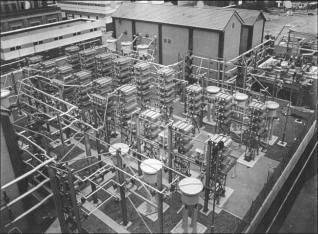
4.5.2 PPS, NPS and ZPS modelling
The PPS and NPS equivalent circuits of a static variable compensator are identical and consist of the compensator transformer in series with the inductive and/or capacitive susceptance of the reactive elements. The admittance is calculated from Figure 4.49(b) using S = P + jQ = VI*, I = YV and P = 0. Thus, the PPS and NPS admittance is given by
where Q is the reactive power output and V is the voltage at the LV side of the compensator transformer. Both Q and V are known from an initial load flow study.
In the ZPS network, the compensator is represented by its transformer leakage impedance only as shown in Figure 4.49(c).
4.6 Sequence modelling of static power system load
4.6.1 Background
The term power system load does not have an agreed and clear meaning in academia or industry and in practice, it can be interpreted to mean many different things by practising engineers. Much research and development has been carried out to define the term load as well as its parameters and characteristics for use in short-term power flow and transient stability studies. However, to my knowledge, the load has received little attention in large-scale network short-circuit analysis. A primary reason for this is that it has been a general practice to ignore the presence of load and calculate the short-circuit current changes in the network due to the short-circuit faults only. This is the case of IEC 60909 and American IEEE C 37.010 standards as will be discussed in Chapter 7. However, as we will see later, the pressures in recent years for increased accuracy and precision in short-circuit calculations resulted in the introduction of new techniques that require the inclusion of the load in the analysis.
It is straightforward to include a model of load equipment in the analysis where this equipment is clearly identifiable because its electrical characteristics would generally be known. For example, a heating load, lighting load or induction motor load, the latter will be covered in detail in Chapter 5, can easily be modelled if one knew how much there is of each component. Nearly all the load components in an industrial power system or a power station auxiliary system would be known. However, in distribution, subtransmission and transmission system short-circuit analysis, the load in MW and MVAr at any given time is that supplied at a major grid supply substation, e.g. 132 kV substation, or a major bulk supply substation, e.g. 33 kV. This load therefore consists of thousands or tens of thousands of components of different types and characteristics and such composition is generally unknown to the network company. The load will contain static components, i.e. those that do not provide a short-circuit contribution to a fault in the host network such as a fixed impedance load. Importantly, from a short-circuit analysis viewpoint, the load will contain a numerous number of single-phase induction motors, three-phase induction motors and embedded large or small scale three-phase synchronous generators all of which will feed a short-circuit current to a fault in the host network. In addition, these load components will be separated from the grid and bulk supply substations by distribution networks. Therefore, the general loads seen at these substations for modelling in large-scale analysis will consist of distribution networks as well as passive and active, i.e. machine, components. Better precision short-circuit analysis should model the contribution of rotating plant, i.e. motors and generators, forming part of the general load at each substation in the network. The sequence modelling of rotating machines is covered in detail in Chapter 5 but we will now restrict our attention to static or passive load as seen from major load supply substations.
4.6.2 PPS, NPS and ZPS modelling
The PPS and NPS model of a passive load supplied radially at a substation that includes the load components and the intervening distribution network can be generally represented as a shunt admittance to earth as follows:
where P and Q is the load supplied in pu MW and pu MVAr and V is the voltage at the substation just before the occurrence of the short-circuit fault, in pu.
The ZPS model of a passive load can be substantially different from the PPS/NPS model. Generally, this model is determined by the presence of low ZPS impedance paths for the flow of ZPS currents such as those provided by star-delta transformers. The ZPS model is therefore the minimum ZPS impedance seen from the supplied substation looking down into the distribution network topology and equipment characteristics including transformer winding connections.
4.7 Three-phase modelling of static power plant and load in the phase frame of reference
4.7.1 Background
In Chapter 6, we describe a short-circuit analysis technique in large-scale power systems in the phase frame of reference. This type of analysis requires the use of three-phase models for power plant and load rather than PPS, NPS and ZPS models. Three-phase models are presented in this section.
4.7.2 Three-phase modelling of reactors and capacitors
The three-phase series impedance and admittance matrix models for series reactors are given in Equations (4.60a) and (4.60b), respectively. Where interphase mutual coupling exists, the series phase impedance matrices given in Equations (4.61a) and (4.61d) apply for unequal and equal interphase couplings, respectively. The corresponding phase admittance matrices are given by
 (4.69a)
in the case of unequal interphase mutual coupling, and
 (4.69b)
in the case of equal interphase mutual coupling, i.e. ZM1 = ZM2 = ZM.
The three-phase shunt admittance matrix of shunt reactors and capacitors was given in Equation (4.62a). For modern varistor protected series capacitors, the current-dependent three-phase series impedance matrix was given in Equation (4.65). The corresponding series phase admittance matrix is given by
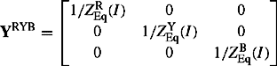 (4.70)
4.7.3 Three-phase modelling of transformers
General
The sequence modelling of single-phase and three-phase transformers of various winding connections was extensively covered in Section 4.2. In three-phase steady state analysis in the phase frame of reference, three-phase models are required. For the purpose of steady state e.g. short-circuit analysis, it is sufficient to model the transformer as a set of mutually coupled windings with a linear magnetising reactance. We will not provide a similar extensive coverage to that in Section 4.2 but will instead present the basic modelling technique of a single-phase two-winding transformer, three-phase transformer banks and a three-limb core three-phase transformer. For the three-phase transformer, only a star-delta winding connection is considered. The principles provide the reader with the information and methodology required to develop a three-phase model for a transformer of any winding connection.
Single-phase two-winding transformers
Figure 4.51(a) illustrates a single-phase two-winding transformer represented as a set of two mutually coupled windings where: Z11(Y11) is winding 1 self-impedance (admittance) and Y11 = 1/Z11; Z22(Y22) is winding 2 self-impedance (admittance) and Y22 = 1/Z22; Z12 = Z21(Y12 = Y21) is mutual impedance (admittance) between windings 1 and 2 and Y12 = 1/Z12; ZHL(YHL) is leakage impedance (admittance) of windings 1 and 2 and YHL = 1/ZHL.
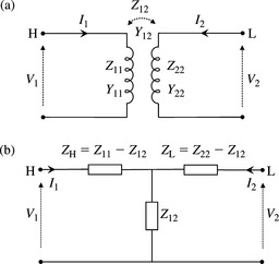
Figure 4.51 Single-phase two-winding transformer: (a) two mutually coupled windings and (b) equivalent circuit
From Figure 4.51(a), we can write
From Equation (4.71), the self-impedance Z11 of winding 1 and the mutual impedance Z12 between the two windings are obtained from the results of an open-circuit test with winding 1 supplied and winding 2 open-circuited and are given by
From Equation (4.72a), the mutual impedance can be expressed as
where V1/V2 is the transformer no-load voltage ratio.
Similarly, the self-impedance Z22 of winding 2 and the mutual impedance Z12 between the two windings can be obtained from the results of an open-circuit test with winding 2 supplied and winding 1 open-circuited. Thus
From Equation (4.73a), the mutual impedance can be expressed as
From Equations (4.72b) and (4.73b), we have
The leakage impedance ZHL between the two windings is obtained from the results of a short-circuit test with winding 1 supplied and winding 2 short-circuited. Thus
Using Equation (4.75a) in Equation (4.71), the leakage impedance ZHL can be expressed in terms of the windings self and mutual impedances as follows:
Having obtained all four elements of the impedance matrix of Equation (4.71), it is more convenient to use the corresponding admittance matrix given by
where
Using Equations (4.73b), (4.74) and (4.75b) in Equations (4.76b), we obtain
and
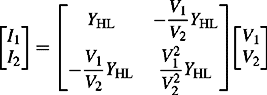 (4.77b)
In the derivation of the above impedance and admittance matrices, we note that, in practice, the only data most likely available are the measured short-circuit leakage impedance and no-load current. The derivation is illustrated using an example.
Example 4.8
Consider a 239 MVA 231 kV/21.5 kV single-phase two-winding transformer having a leakage reactance of 15% and a no-load current of 0.5% whether measured from the high or low voltage sides. Thus, Z11 = Z22 = 1/0.005 = 200 pu. Equation (4.71) can be represented by the equivalent circuit of Figure 4.51(b) where the self-impedance of a winding is defined as the sum of its leakage impedance and the mutual impedance, i.e. in per-unit, Z11 = Z22 = ZH + Z12 = ZL + Z12 giving ZH = ZL. Since ZH = ZL « Z12, the short-circuit leakage impedance is given by ZHL = ZH + ZL giving ZH = ZL = 0.075 pu. Ignoring the magnetising losses and the resistive part of the leakage impedance, the mutual reactance is equal to jX12 = j200 – j0.075 = j199.925 pu. Therefore, the impedance and admittance matrices, in pu, are given by
The difference between the self and mutual reactances is the very small value of 1/2 the leakage reactance. This results in very small differences between the self and mutual susceptances and necessitates calculations to at least six or seven decimal places if the important leakage reactance is not to be lost. The corresponding reactance and susceptance matrices in ω are given by
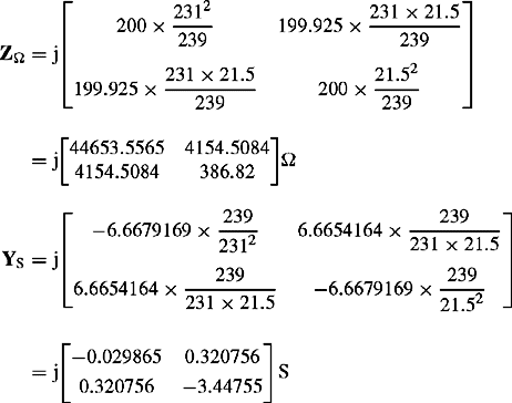
The admittance matrix could also be calculated using Equation (4.77b). The leakage impedance referred to the HV side is equal to ![]() . The elements of the admittance matrix of Equation (4.77b) are calculated using Equation (4.77a).
. The elements of the admittance matrix of Equation (4.77b) are calculated using Equation (4.77a).
The above approach can easily be extended to single-phase three-winding transformers where the dimension of the admittance matrix of Equation (4.76a) becomes 3 × 3. Obviously, we now have three self admittances, three mutual admittances and three short-circuit leakage admittances. This is a simple exercise in algebra left for the reader to derive the admittance equations following a similar method to the two-winding case.
Three-phase banks two-winding transformers (no interphase mutual couplings)
Consider a large two-winding star–delta transformer constructed as three single-phase banks as shown in Figure 4.52.
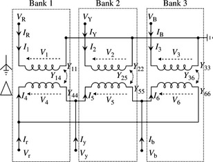
In such an arrangement, there is negligible or no interphase coupling between the three phases. Using the admittance matrix given in Equation (4.76a) for each phase and Figure 4.52, the admittance matrix equation that relates the winding currents and voltages for the three-phases is given by
 (4.78a)
or
Equation (4.78b) applies to a two set of three-phase windings irrespective of the type of winding connection. Thus, for our star–delta transformer, the three-phase nodal admittance matrix that relates the nodal currents and voltages can be derived from the relationship between the winding currents and voltages, and the nodal currents and voltages. With all nodal voltages being with respect to the reference earth, the relationship between the winding and nodal voltages is found by inspection from Figure 4.52 as follows:
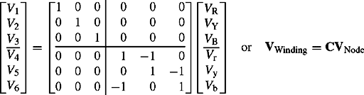 (4.79a)
where C is defined as the connection matrix. Similarly, the relationship between the nodal and winding currents is found by inspection from Figure 4.52 and is given by
 (4.79b)
Using Equations (4.79a) and (4.79b) in Equation (4.78b), we obtain
where
Denoting the star-connected winding as H and the delta-connected winding as L, Equation (4.80a) can be written in partitioned form as follows:
Using Equation (4.77a), it can be shown that the self and mutual admittance matrices of Equation (4.81a) are given by
 (4.81b)
where YHL14 = 1/ZHL14 and so on.
In the per-unit system with both the star and delta voltages equal to one per unit, the effective turns ratio on the delta side is ![]() . If the three phases of the transformer are considered identical, i.e. having identical leakage admittances that is
. If the three phases of the transformer are considered identical, i.e. having identical leakage admittances that is ![]() ,then using Equation (4.81), Equation (4.80b) becomes
,then using Equation (4.81), Equation (4.80b) becomes
 (4.82)
To allow for the effect of off-nominal tap ratio, e.g. on the star side, then according to Equation (4.13a), the terms of the self admittance YHH should be divided by ![]() whereas the terms of the mutual admittances YHL and
whereas the terms of the mutual admittances YHL and ![]() should be divided by tHL.
should be divided by tHL.
The reader is encouraged to show that the nodal admittance matrix of a two-winding star–star transformer with both neutrals solidly earthed and no interphase mutual couplings has the form as the winding admittance given in Equation (4.78a). Using these principles, the reader can easily obtain the nodal admittance matrix for any winding connections of a three-phase banks of transformers.
Three-phase common-core two-winding transformers (with interphase mutual couplings)
For three-phase 3-limb, 5-limb or shell-type core transformers, interphase mutual couplings exist and these are generally asymmetrical, as can be expected from Figures 4.28-4.30, between the outer-limb phases and the phases connected to adjacent limbs. However, in practice, little or no information is available on these asymmetrical coupling affects. Standard transformer test certificates include the normally measured parameters, i.e. the PPS and ZPS impedances and the magnetising current from which the magnetising impedance is calculated. Since the PPS and ZPS impedances are generally different, this implies that equal interphase mutual couplings exist in the three-phase admittance matrix. The asymmetrical interphase coupling effects may also be indirectly averaged out by their short-circuit measurement procedures as described in Section 4.2.10. Figure 4.53 illustrates a common-core star–delta transformer where each phase winding is coupled to all other phase windings and where windings 1 and 4, 2 and 5, and 3 and 6, are wound on the same limb. With the assumption of full flux symmetry, we obtain a 6 × 6 winding admittance matrix that consists of four 3 × 3 symmetrical submatrices. The corresponding nodal admittance matrix can be obtained using Equation (4.80b).
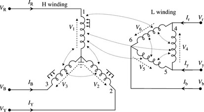
However, since in nearly all practical situations only sequence and magnetising impedances are available, we will present a different technique for the formulation of the transformer three-phase model. The technique is based on using the known PPS and ZPS leakage impedances, ignoring the magnetising impedances for now. To illustrate the technique, we consider the star-delta transformer of Figure 4.53 with a tap-changer on the star side. In Figure 4.53, phase R of the star winding is assumed symmetrically coupled with phases Y and B of the star winding on different limbs, with phase ‘ry’ on the delta winding on the same limb, and with phases ‘rb’ and ‘by’ on the delta winding on different limbs. Similar symmetrical couplings are assumed for other phases. The PPS and NPS equivalent circuits are shown in Figure 8.4(a) and (b). The ZPS equivalent circuit is shown in Figure 4.12(g) with ZE = 0. Equation (4.13a) corresponds to Figure 4.8(c) where the transformer winding phase shift of 30° for Yd1 and −30° for Yd11 connections was neglected. In the derivation to follow, we denote the star side as H and the delta side as L. Therefore, denoting the phase shift as φ and letting all impedances be expressed in pu, it can be shown that the PPS and NPS nodal admittance matrices of Figures 4.8(a) and (b) are given by
 (4.83a)
 (4.83b)
and the ZPS nodal admittance matrix of Figure 4.12(g) with ZE = 0 is given by
 (4.83c)
Equations (4.83a), (4.83b) and (4.83c) can be assembled to obtain the transformer sequence admittance matrix, including sequence current and voltage vectors, as follows:
 (4.84a)
or
 (4.84b)
It should be noted that ![]() . The phase admittance matrix is obtained using the sequence to phase transformation matrix H noting that in pu, the effective delta winding turns ratio is
. The phase admittance matrix is obtained using the sequence to phase transformation matrix H noting that in pu, the effective delta winding turns ratio is ![]() . Thus
. Thus
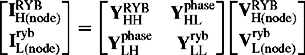 (4.85a)
 (4.85b)
Therefore, using Equations (4.84) in Equations (4.85b) and (4.85c), the self (H and L windings) and mutual (H–L and L–H windings) phase admittance matrices are given by
 (4.86a)
 (4.86b)
 (4.87a)
and
It should be noted that for star–star and delta–delta connected two-winding transformers, φ = 0 or φ = 180°. However, for the Yd1 transformer of Figure (4.53), φ = 30° and the mutual phase admittance matrices become
 (4.87c)
The transformer PPS magnetising impedance is generally available from the open-circuit test. The ZPS magnetising impedance may also be available from a direct test for some transformers. Alternatively, where it is not available, it can be estimated from the measured PPS and ZPS leakage impedances as discussed in Section 4.2.9. Where no measured ZPS leakage impedance is available, the magnetising impedance and the ZPS leakage impedance may be estimated as discussed in Section 4.2.9. The PPS magnetising impedance is so high in comparison with the PPS leakage impedance that it may be connected on the high voltage side of the transformer with practically negligible error. The ZPS magnetising impedance is also better and more correctly connected nearer the high voltage side of the transformer because the LV winding is wound nearer the core but the HV winding is wound on the outside over the LV winding. Therefore, the effect of this connection is to modify the sequence admittance matrix![]() and the corresponding phase admittance matrix
and the corresponding phase admittance matrix![]() to
to
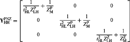 (4.88a)
 (4.88b)
where
and ![]() and
and ![]() are the PPS and ZPS magnetising impedances, respectively.
are the PPS and ZPS magnetising impedances, respectively.
Three-phase models for other transformer winding connections including three-winding transformers that result in a 9 × 9 nodal phase admittance matrix can be derived using a similar technique.
4.7.4 Three-phase modelling of QBs and PSs
In some special analysis, both the shunt and series transformers of QBs and PSs need to be explicitly modelled as three-phase devices. However, for most steady state e.g. unbalanced short-circuit analysis on the external network to which these equipment are connected, the two transformers may be combined into the same single model. Similar to a three-phase transformer with symmetrical interphase mutual couplings, we will make use of the PPS and ZPS impedances and equivalent circuits of the combined transformers to derive the three-phase admittance matrix that relates the input and output phase currents and voltages. Therefore, using Figures 4.37(a), 4.39(a) and (b) as well as the sequence admittance Equations (4.56a), (4.57a) and (4.57b), the nodal sequence admittance matrix including sequence current and voltage vectors is given by
 (4.89a)
or
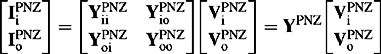 (4.89b)
where ![]() and
and ![]() are the PPS and NPS complex turns ratios and
are the PPS and NPS complex turns ratios and ![]() and
and ![]() are their conjugates.
are their conjugates.![]() is given in Equations (4.54b) and (4.55b) for a QB and a PS, respectively and
is given in Equations (4.54b) and (4.55b) for a QB and a PS, respectively and ![]() is given in Equation (4.57a). Therefore, using YRYB = HYPNZ H−1 it can be shown that the nodal phase admittance matrix is given by
is given in Equation (4.57a). Therefore, using YRYB = HYPNZ H−1 it can be shown that the nodal phase admittance matrix is given by
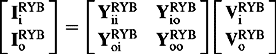 (4.90a)
where
 (4.90b)
 (4.90c)
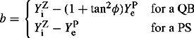 (4.90d)
and
 (4.91)
 (4.92a)
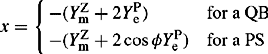 (4.92b)
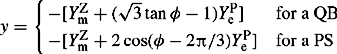 (4.92c)
 (4.92d)
4.7.5 Three-phase modelling of static load
Static three-phase load was represented by equal PPS and NPS impedances or admittances as given by Equation (4.68) and a ZPS impedance or admittance as described in Section 4.6.2. The sequence admittance matrix of the load is given by
 (4.93a)
The corresponding three-phase admittance matrix is calculated using ![]() giving the following balanced three-phase admittance matrix
giving the following balanced three-phase admittance matrix
 (4.93b)
In the special case where the ZPS admittance ![]() is equal to the PPS admittance
is equal to the PPS admittance ![]() ,then the load can be represented as three shunt admittances as follows:
,then the load can be represented as three shunt admittances as follows:
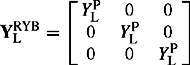 (4.93c)
[1] ISBN 0-906048-47-8The Electricity Council. ‘Power system protection’, Vol. 1, ‘Principles and Components’. 1981.
[2] Arrilaga J., et al. Computer Modeling of Electrical Power Systems. John Wiley & Sons; 1983. 0-471-10406-X.
[3] Grainger J.J. Power System Analysis. McGraw-Hill Int. Ed.; 1994. 0-07-061293-5.
[4] Weedy B.M. Electric Power Systems. John Wiley & Sons; 1967. 0-471-92445-8.
[5] Bratton E., et al. Tertiary windings in star/star connected power transformers. Electrical Power Engineer. June 1969:6-9.
[6] Riedel, P., “Modeling of zigzag-transformers in the three-phase systems’, Institute for Electrical Engineering D-3000 Hanover 1, FRG, pp. T3/1-T3/9.
[7] No. 7Chen Mo-Shing, et al. Power system modeling. IEE Proceedings. Vol. 62. July 1974:901-915.
[8] No. 8Laugton M.A. Analysis of unbalanced polyphase networks by the method of phase coordinates. IEE Proceedings. Vol. 115. August 1968:1163-1171.
[9] Bowman W.I., et al. Development of equivalent Pi and T matrix circuits for long untransposed transinission lines. IEEE Summer General Meeting and Nuclear Radiation Effects Conference. Toronto, Ont. June 1964:625-631.
[10] Jimenez, R., et al., ‘Protecting a 138 KV phase shifting transformer: EMTP modelling and model power system testing’, 2002, 1–15.
[11] Mahseredjian J., et al. Superposition technique for MOV-protected series capacitors in short-circuit calculations. IEEE Transactions On Power Delivery. July 1995;Vol. 10(No. 3):1394-1400.
[12] Goldworthy D.L. A linearised model for MOV-protected series capacitors. IEEE PES Transactions Paper 86 SM 357-8. Mexico City. 1986.