Programming Model

Even if an iterative approach could be used in MapReduce , there are two impediments: the same data could be processed on more iterations (because data remains unchanged) and the stopping condition that checks whether a fixed point occurred (namely, to check if the same data is processed on two successive iterations).

The main architecture and functionalities of Hadoop are kept in HaLoop, which works as follows: the input and the output of the jobs are stored in HDFS. There is a master node that coordinates the slave nodes. When the client sends its jobs, the master node allocates a particular number of parallel tasks that need running over the slave nodes. In each slave node, a tracker monitors the execution of the jobs and communicates with the master node. There could be a map task or a reduce task. Figure 15-1 illustrates the similarities and differences between Hadoop and HaLoop.

Figure 15-1. Hadoop vs. HaLoop

MapReduce programs are optimized by HaLoop through catching the intermediary results between MapReduce jobs. This ends if a fixed point is achieved (i.e., two consecutive iterations have the same result).

In HaLoop it is possible to have an approximate fixed point in which the difference between the outputs of two successive iterations is less than a value given by the user, or the maximum number of iterations is achieved. The two types of approximate fixed points are useful in machine learning applications.

In HaLoop programs, the work of the programmer is to specify the loop body (i.e., one or more map-reduce steps). Specifying the termination rule and the data invariant for the loop is optional. The map and reduce functions are similar to those of standard MapReduce. In a HaLoop program, the following functions should be used.

• The map function takes as input a pair (key, value) and outputs an intermediate pair (in_key, in_value);

• The reduce function takes as input the intermediate pair (in_key, in_value) and outputs the final pair (out_key, out_value). There is a new parameter used for cached invariant values corresponding to in_key.

• AddMap and AddReduce contain a loop body in which there are multiple map-reduce steps. Every map/reduce function has a corresponding integer that shows the order of the step associated with AddMap/AddReduce.

HaLoop’s default state is dedicated to testing if the current iteration is equal with the previous iteration. In this way it is determined when the computation should be terminated. To specify a specific point as a condition, the programmer should use these functions.

• The SetFixedPointThreshold function fixes a bound on the distance that is situated between the current iteration and the next iteration. The computation continues while the threshold is not excedeed and the fix point is not reached.

• The ResultDistance function computes the distance between out_values sets that share the same out_key. v _i is an out_value set from the reducer output of the current iteration. v _i-1 an out_value set from the previous iteration’s reducer output. The distance between the reducer outputs of the current iteration, I, and the last iteration, i-1, represents the sum of ResultDistance for each of the keys.

• The SetMaxNumOfIterations function provides further control of the loop termination condition. HaLoop terminates the job if the maximum number of iteration has been executed, taking into consideration the current and previous iteration’s outputs. SetMaxNumOfIterations acts as guidance to implement a simple for-loop.

To specify the control inputs, the programmer has to acknowledge the following:

• The SetIterationInput function associates an input source with a specific iteration, since the input files to different iterations may be different. Figure 15-2 illustrates that at each iteration, i+1, is the input.

  

  Figure 15-2. The boundary between an iterative application and the framework illustrated in Figure 15-1. HaLoop knows and controls the loop, while Hadoop only knows jobs with one map-reduce pair.

• The AddStepInput function associates an additional input source with an intermediate map-reduce pair situated in the body of the loop. The output resulted from the preceding map-reduce pair is always in the input of the next map-reduce pair.

• The AddInvariantTable function specifies an input a table (under the form of HDFS file) that is loop-invariant. After the code executes, HaLoop caches this table on cluster nodes.

The current programming interface is sufficient to express a variety of iterative applications. Figure 15-2 depicts the main difference between HaLoop and Hadoop, from the application’s point of view. With HaLoop, the user of the application specifies the loop settings and the framework that controls the loop execution; but in Hadoop, it is the application’s responsibility to control the loops.

Loop-Aware Task Scheduling

From this point, we focus on the HaLoop task scheduler . The scheduler provides potentially better schedules for iterative programs, which Hadoop’s scheduler is not capable of offering.

Inter-Iteration Locality

The high-level goal of HaLoop’s scheduler is to place the maps and to reduce the tasks that can occur on the same physical machines in different iterations, but access the same data. Using this approach, data can be more easily cached and reused between the respective iterations.

The scheduling of iteration 1 is no different than it is in Hadoop. In the join step of the first iteration, the input tables are L and R ₀. Three map tasks are executed, each of which loads a part of one or the other input data file (e.g., file split). As in Hadoop, the mapper output key is hashed to reduce the task to which it should be assigned. After this, three reduce tasks are executed, each of which loads a partition of the collective mapper output. In Figure 15-3, the reducer denoted with R ₀₀ processed the mapper output keys whose hash value is 0. The R ₁₀ reducer processes the keys with hash value 1, and the R ₂₀ reducer will process the keys with hash value 2.

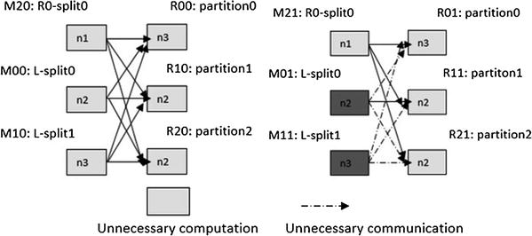
Figure 15-3. A schedule exhibiting inter-iteration locality. Tasks processing the same inputs on consecutive iterations are scheduled to the same physical nodes.

The scheduling of the join step of iteration 2 has the advantage of inter-iteration locality, which means that the task (either a mapper or a reducer) that processes specific data partition D is scheduled on the physical node that D is processed in iteration 1.

The schedule in Figure 15-5 provides the feasibility to reuse loop-invariant data from past iterations. Because L is loop invariant, mappers M ₀₁ and M ₁₁ would compute identical results to M ₀₀ and M ₁₀. There is no need to recompute these mapper outputs or to communicate them to the reducers. In iteration 1, if reducer input partitions 0, 1, and 2 are stored on nodes n3, n1, and n2, respectively, then in iteration 2, L need not be loaded, processed, or shuffled again. In that case, in iteration 2, only one mapper M ₂₁ for R ₁-split 0 needs to be launched, and thus the three reducers will only copy intermediate data from M ₂₁. With this strategy, the reducer input is no different, but it now comes from two sources: the output of the mappers (as usual) and the local disk.

We refer to the property of the schedule in Figure 15-3 as the inter-iteration locality. Let d be a file split (mapper input partition) or a reducer input partition. Let T _d ⁱ be a task consuming d in iteration i. Then we say that a schedule exhibits inter-iteration locality if for all i > 1, and T _d ⁱ and are assigned to the same physical node if exists. The goal of task scheduling in HaLoop is to achieve inter-iteration locality. To achieve this goal, the only restriction is that HaLoop requires that the number of reduce tasks should be invariant across iterations, so that the hash function assigning mapper outputs to reducer nodes remains unchanged.

Experimental Tests and Implementation

HaLoop supports iterative and recursive data analysis tasks as mainly recursive joins. These joins could be map joins (for example, they are used in a k-means algorithm) or reduce joins (for example, they are used in a PageRank algorithm). The key to HaLoop is caching loop-invariant data to slave nodes, and reutilizing them between iterations.

HaLoop is available at http://haloop.googlecode.com/svn/trunk/haloop .

To configure a cluster in HaLoop, we take the same steps as in Hadoop. The difference between clusters in Hadoop and HaLoop is that local mode and the pseudo-distributed mode are not supported by HaLoop, but it is supports real distributed mode.

To run the examples, first compile them.

% ant -Dcompile.hs=yes examples

And then copy the binaries to dfs.

% bin/hadoop fs -put examples

Create an input directory with text files.

% bin/hadoop fs -put my-data in-dir

Now, as practice, modify the word count examples in Chapter 13 (see the “Hadron” section), adding AddMap and AddReduce as described earlier, and run the word-count example as follows.

% bin/hadoop pipes -conf pathfile/word.hs  -input in-dir -output out-dir

Summary

This chapter presented HaLoop, an improvement for Hadoop proposed and implemented by Yingyi Bu et al. It supports iterative and recursive data analysis tasks, which brings

• a loop-aware task scheduler

• loop-invariant data caching

• caching for efficient fixpoint verification