Contiki-NG comes with rich network-stack features to allow communication with others. In this chapter, we will explore the available network features on the Contiki-NG platform. Several scenarios will be provided to enable practice with implementing projects-based Contiki-NG, either in physical motes or in mote simulations.
Networking in Contiki-NG
Working with network simulation using COOJA
IPv6 networking
Routing on Contiki-NG
IPv6 Multicast
Working with Contiki-NG NullNet
Working with a 6LoWPAN network
Building a RESTful server for Contiki-NG
Networking in Contiki-NG
Network layer (NETSTACK_NETWORK)
MAC layer (NETSTACK_MAC)
RDC (Radio Duty Cycling) layer (NETSTACK_RDC)
Radio layer (NETSTACK_RADIO)
Contiki-NG Network Protocol stack
Application layer: http-socket.c, websocket.c, websocket-http-client.c, and mqtt.c
Transport: udp-socket.c and tcp-socket.c
Network & Routing: uip6.c and rpl.c
MAC: mac.c and csma.c
NETSTACK code implementations in Contiki-NG
Network Layer
Contiki-NG relies on an IPv6 stack. All TCP/UDP sockets in Contiki-NG use uIP (uip.h and uip6.c from <contiki-ng>/os/net/ipv6), which implements for IP, UDP, and TCP protocols in minimized models.
Currently, the network layer contains two sublayers, the upper IPv6 layer and the lower adaptation layer. These sublayers run on the top of IEEE 802.15.4 with Time-Slotted Channel Hopping (TSCH).
DODAG routing graph form
Upward: from any node toward a root
Downward: from the root to any node
Any-to-any: flows among arbitrary pairs of nodes in the DODAG graph
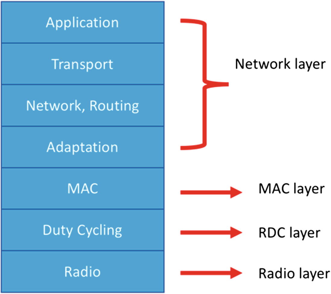
For RPL implementation, Contiki-NG provides RPL classic and RPL lite. RPL classic is the original Contiki RPL implementation, called ContikiRPL. I recommend you read the ContikiRPL paper on this site: http://www.diva-portal.org/smash/get/diva2:1042739/FULLTEXT01.pdf .
You can find code implementations for both RPL classic and RPL lite in Contiki-NG. RPL classic can be found at /net/rpl-classic and RPL lite at /net/rpl-lite from the Contiki-NG code root. See them in Figure 6-4.
The nullnet library from Contiki-NG can be used to test your packet from upper to lower layers. This library can be found at <contiki-ng>/os/net/nullnet.
MAC Layer
The MAC layer is designed to address collisions in packet traffic and to apply back-off if there is traffic. Contiki-NG applies CSMA/CA (Carrier Sense Multiple Access with Collision Avoidance) for MAC layer implementation. Contiki-NG uses CSMA/CA on the IEEE 802.15.4 protocol. You can see program implementation in the <contiki-ng>/os/net/mac folder.
In the CSMA/CA algorithm, a mote will sense the medium before sending packets. If another mote is sending a packet, the mote will apply back-off with a certain value depending on the RDC layer. If the medium is free, the mote will send packets that have been prepared by the network layer.
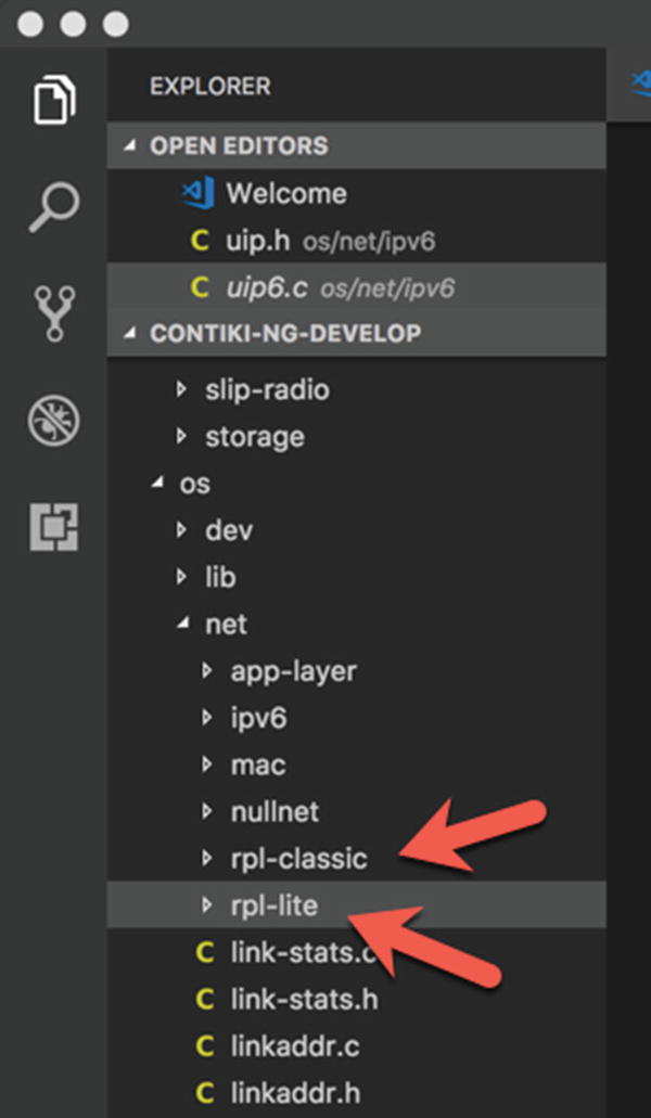
RPL classic and lite libraries in Contiki-NG
RDC Layer
The Radio Duty Cycling (RDC) layer saves energy by allowing a node to keep its radio transceiver off most of the time. Contiki-NG supports the ContikiMAC protocol based on the principles behind low-power listening. ContikiMAC uses Time Slotted Channel Hopping (TSCH) that is a part of the MAC layer of the IEEE 802.15.4e-2012 amendment.
Radio Layer
The radio layer is the lowest layer in the Contiki-NG NETSTACK. The radio layer is handled by radio module from the Contiki-NG mote. Most radio layers work on the IEEE 802.15.4 protocol mechanism.
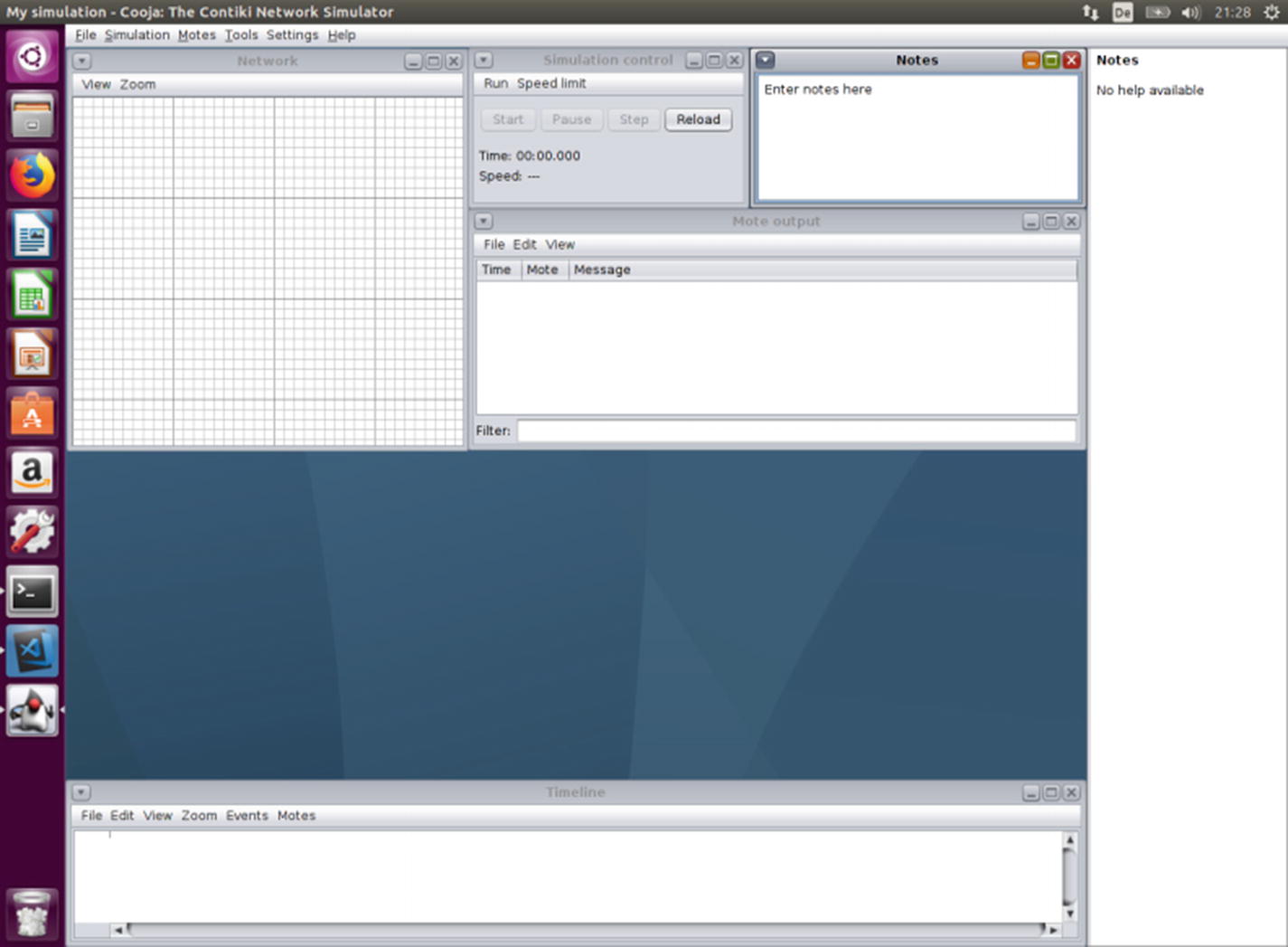
Network Simulation Using COOJA
In Chapter 1, we learned how to work with COOJA to build a Contiki-NG simulation. In this section, we will continue to apply COOJA to create a network simulation. For this simple demo, we will use the same scenario as in Chapter 4. We will perform broadcasting among Contiki-NG motes.
Create a simulation project.
Add a UDP server mote.
Add UDP client motes.
Run the simulation.
Each task will be performed in the following sections.
Creating Simulation Project
The first step is to create a simulation project using COOJA. From your platform Terminal, you can run the COOJA tool. For instance, I run it from Ubuntu Linux. You can type these commands:
COOJA application
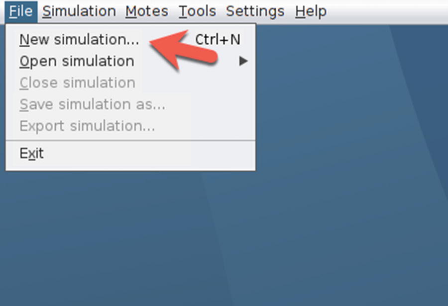
Create a new simulation in COOJA
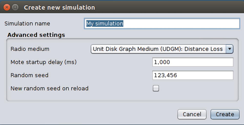
Fill in simulation name and other settings
If done, you can click the Create button to create the simulation.
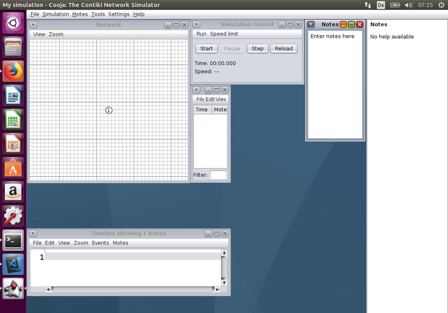
After that, COOJA will create a new simulation for you. Figure 6-8 shows a simulation dashboard from COOJA. Now you are ready to configure the simulation.
Cooja with simulation dashboard
Adding UDP Server Mote
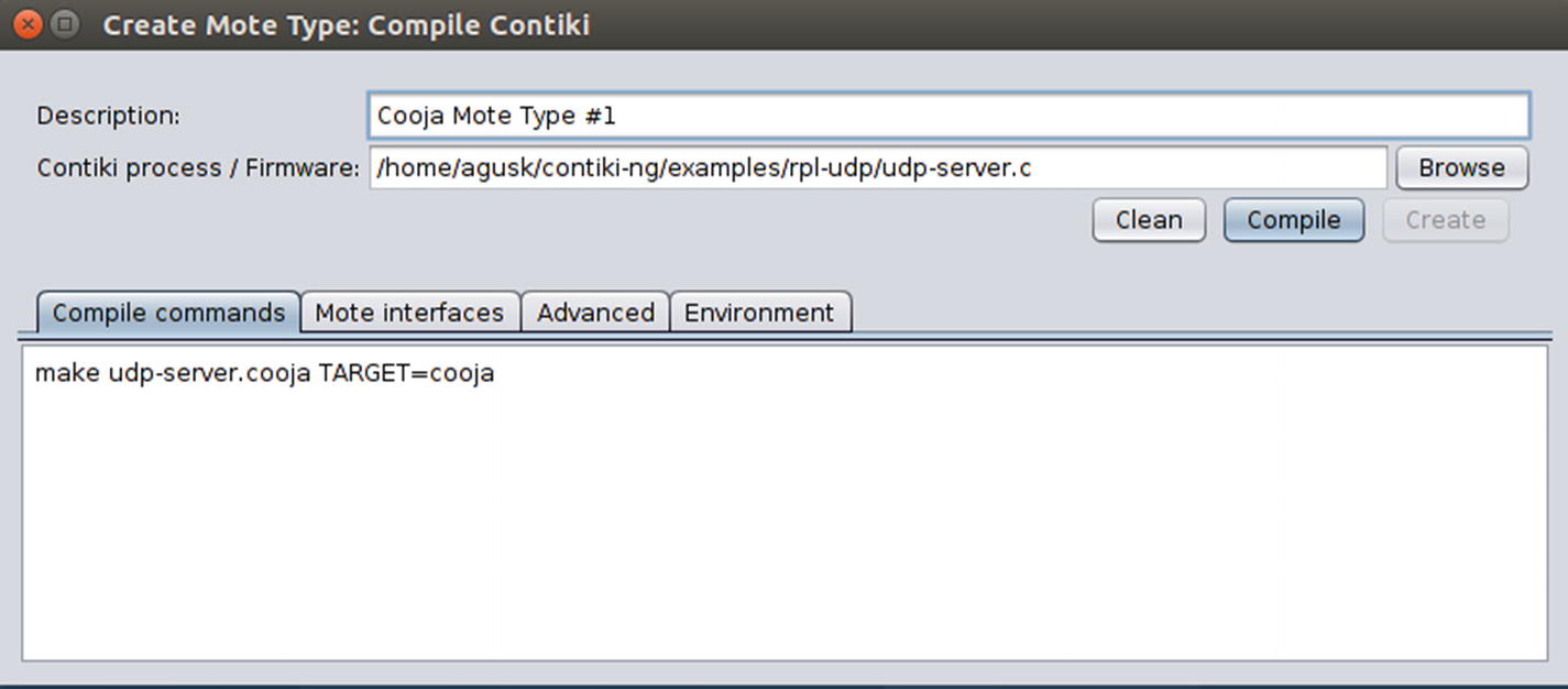
In this section, we will add a mote as the UDP server. This mote will listen to incoming messages. Once a message is received from a client, the UDP server will reply by sending that message. For the demo, we will use a mote with the Sky platform type.
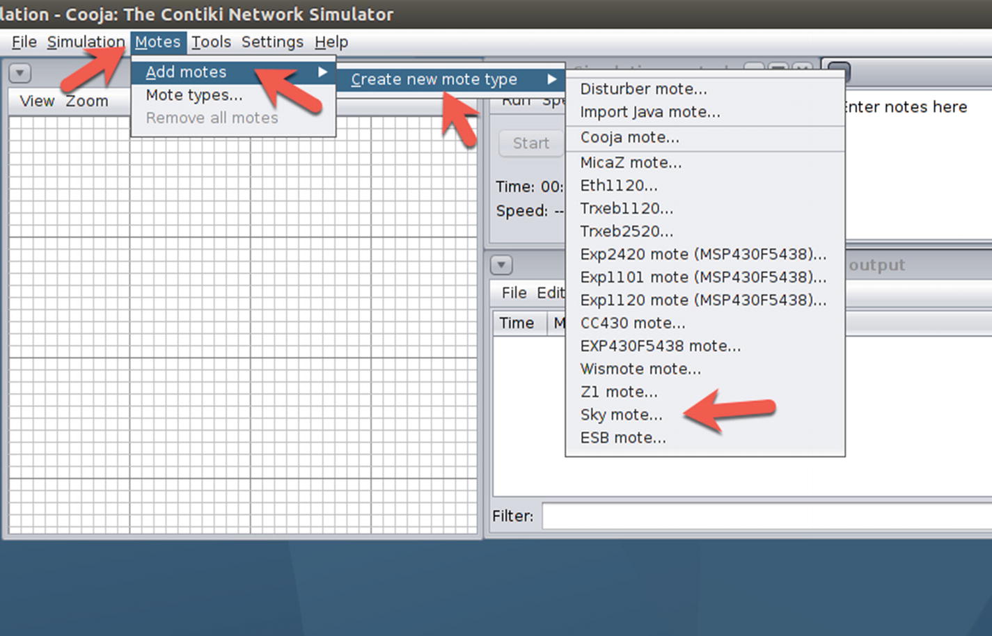
Adding a new mote
Add the UDP server mote
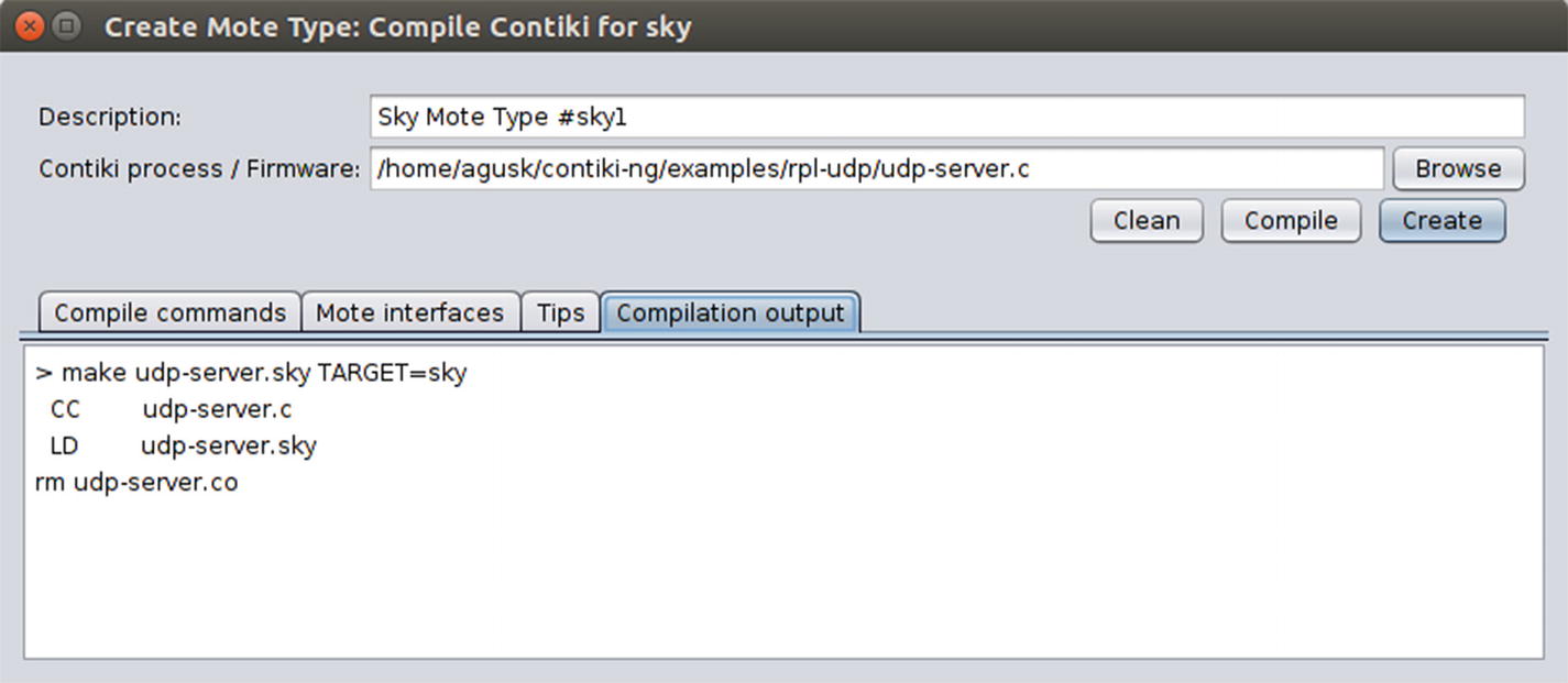
Compile the UDP server mote
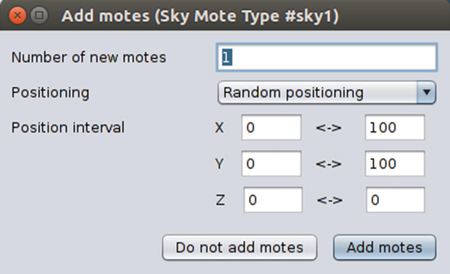
Configure the mote number and its position
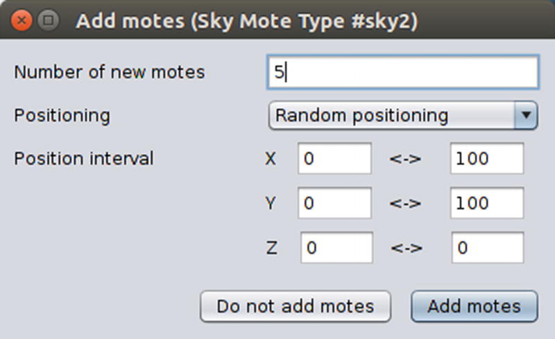
In this scenario, we only add one mote for the UDP server. You can fill in 1 for the “Number of new motes” field and select Random positioning for the “Positioning” dropdown.
UDP server is deployed on COOJA
Next, we will add some motes for the UDP client. We will perform this task in the next section.
Adding UDP Client Motes
After we have created one UDP server mote, we can create some UDP client motes. For this demo, we will add five motes. To add a new mote, you perform this task as in the previous section.
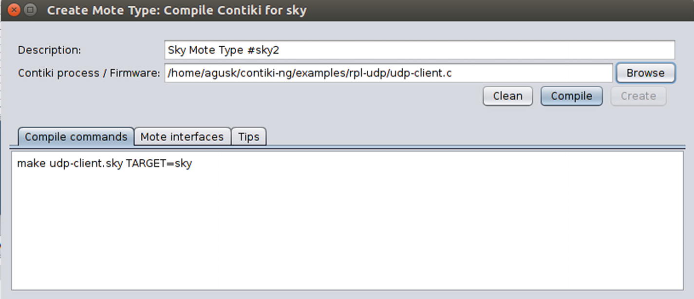
Adding UDP client mote
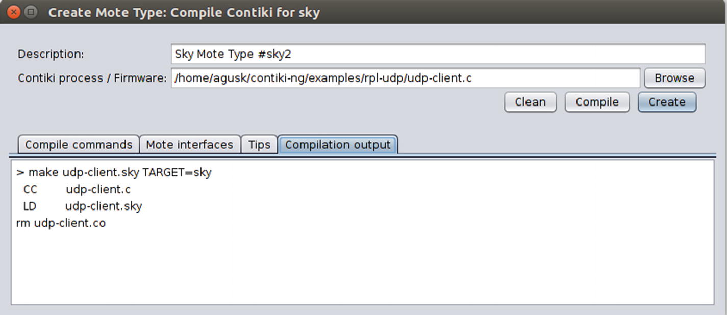
Compiling UDP client mote
Adding five UDP client motes
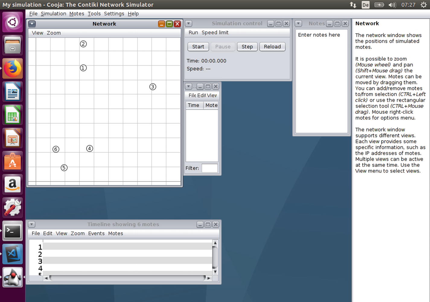
Deployed UDP client motes on COOJA
Running a Simulation
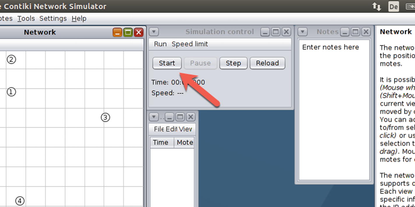
Starting a simulation
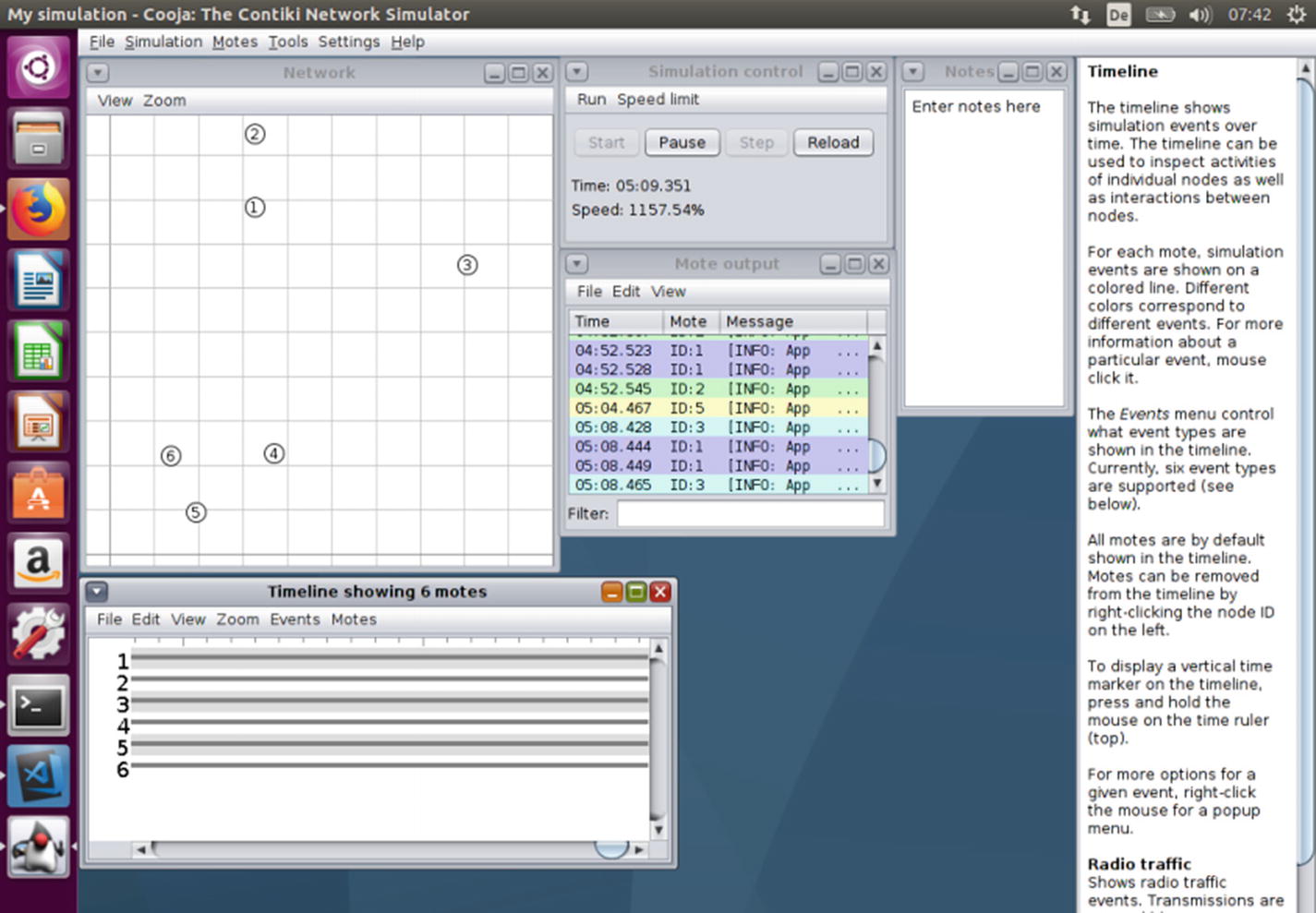
A simulation is running on COOJA
If the distance between motes is far, some motes probably won’t connect or receive UDP messages. You can change the mote location so each mote can be connected.
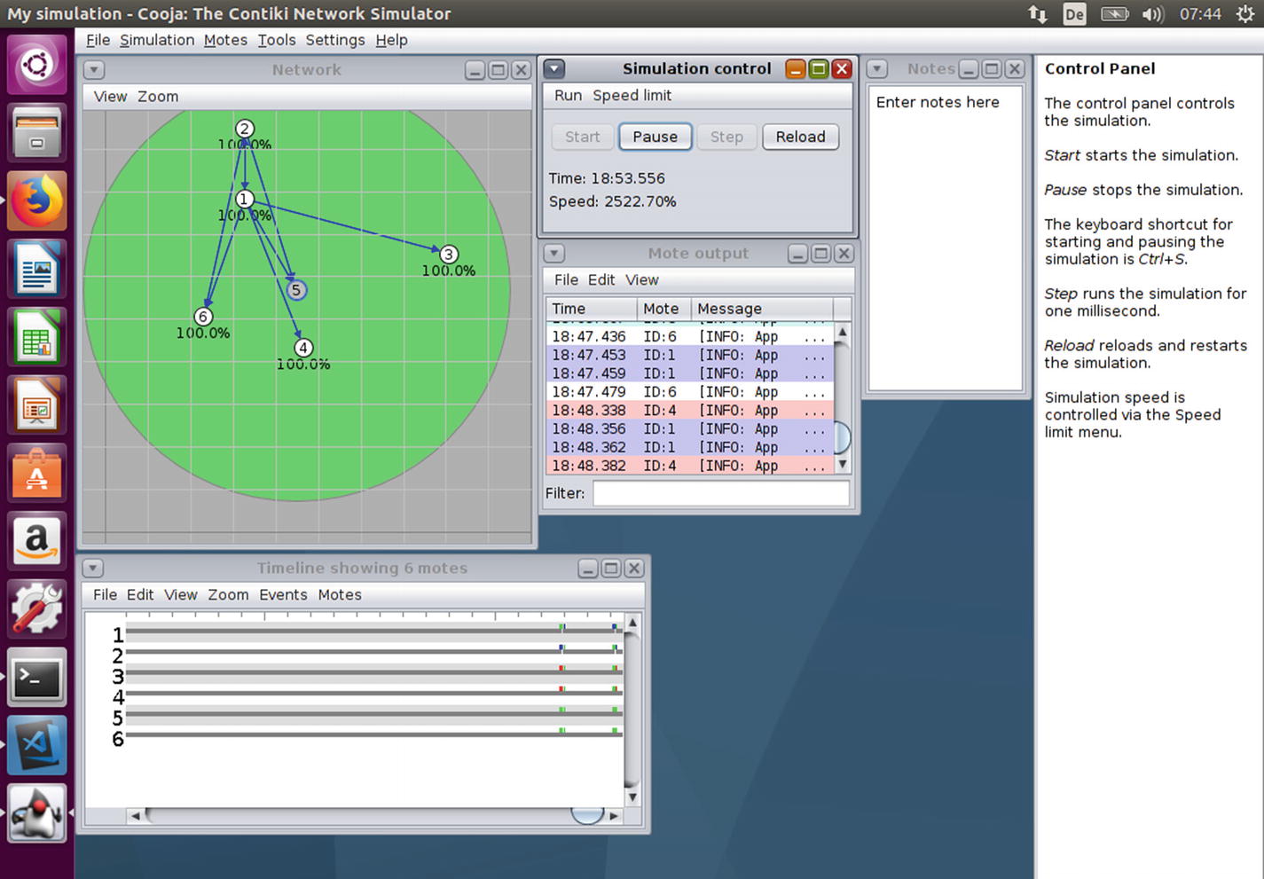
Changing mote location
IPv6 Networking
IPv6 (Internet Protocol Version 6) is the Internet’s next-generation protocol, designed to replace the current protocol, IP Version 4 (IPv4). Most network systems still use IPv4 to communicate with other systems. Sample IP addresses from IPv4 and IPv6 are shown here:
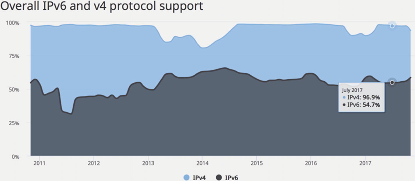
Comparing IPv4 and IPv6 protocol support worldwide
For more learning material about IPv6, I recommend you read some textbooks or technical articles related to IPv6 technology. This book does not cover IPv6 technology in any depth.
Contiki-NG can work with an IPv6 network by default. Contiki-NG projects provide uIP as the network stack implementation for IP, UDP, and TCP protocols included in the basic ICMP protocol. The uIP library can run on constrained devices, such as Tmote Sky/TelosB, TI cc26xx/cc13xx, Firefly, RE-mote, and Orion.
For our IPv6 demo on Contiki-NG, we can perform testing using a Contiki-NG shell (NG shell). To enable an NG shell for your program, you should add a shell module to your Makefile file:
Then, you can compile and upload to your mote. Since the shell module needs more space, you should use a mote platform that can handle NG shell spaces. In this demo, I use a TI CC2650 LaunchPad board.
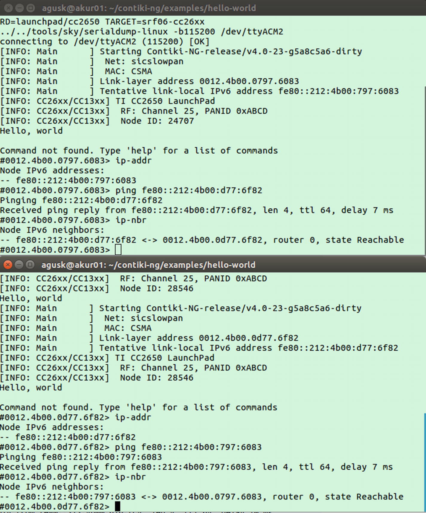
For testing, we need two motes at least. Upload your project; for instance, hello-world with NG shell enabled. After uploading Contiki-NG firmware onto the boards , we can remote into the NG shell from a serial terminal.
For instance, I remote into the TI CC2650 LaunchPad via the /dev/ttyACM0 port:
Open a new Terminal window. Then, perform a serial remote on the second mote. For instance, my second mote runs on the /dev/ttyACM2 port:
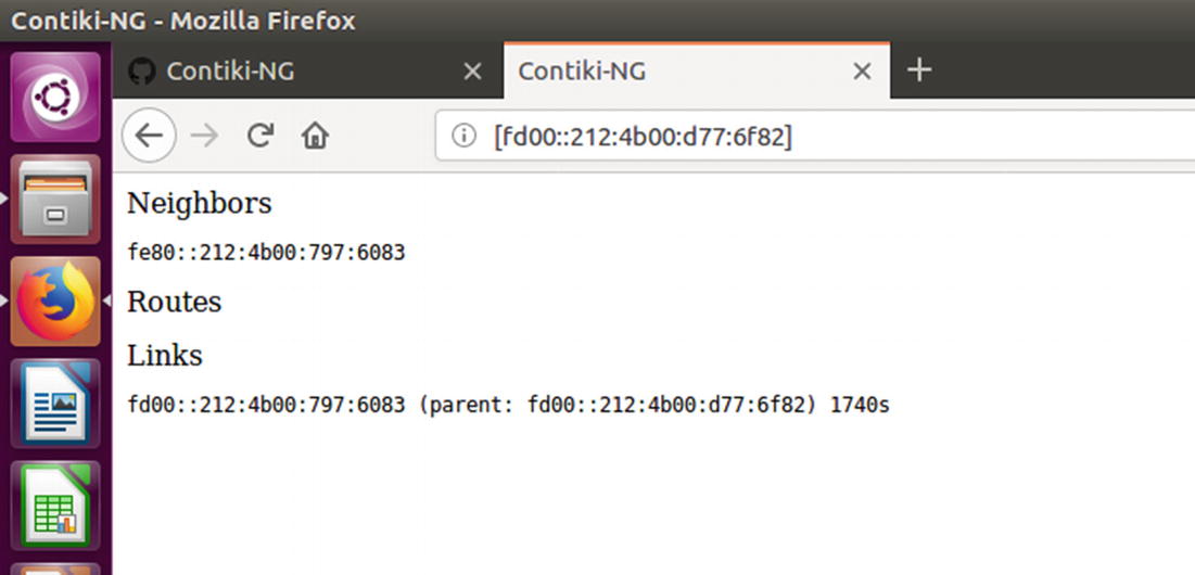
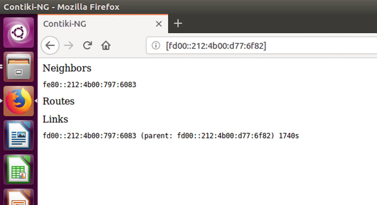
After connecting to the NG shell, we can perform some tests related to IPv6 operations. You can check the current IPv6 address on each mote. You can type this command in the NG shell:
You should see an IPv6 address for each mote. Next, you can perform a ping to one of the motes. For instance, I perform a ping on a mote with the IPv6 address fe80::212:4b00:d77:6f82:
You should get a response from ping operations. Last, our mote can discover its neighbor. By default, Contiki-NG enables UIP_ND6_AUTOFILL_NBR_CACHE to be discoverable. You can perform this command to discover a mote’s neighbor:
IPv6 testing via Contiki-NG shell
Routing on Contiki-NG
Routing is the process of moving packets across a network from source to destination. This process is usually performed by dedicated network devices, such as routers and computers. Routing is a key feature of the Internet. Routing topics as a research area is still popular. Some researchers propose algorithms to address routing problems. In this section, we will review routing and how to implement it in the Contiki-NG platform.
Introducing Basic Routing
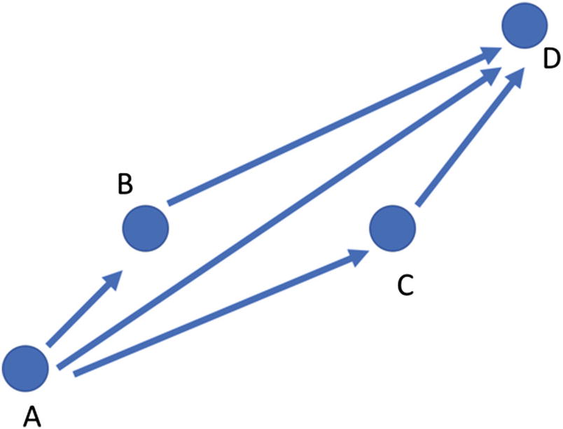
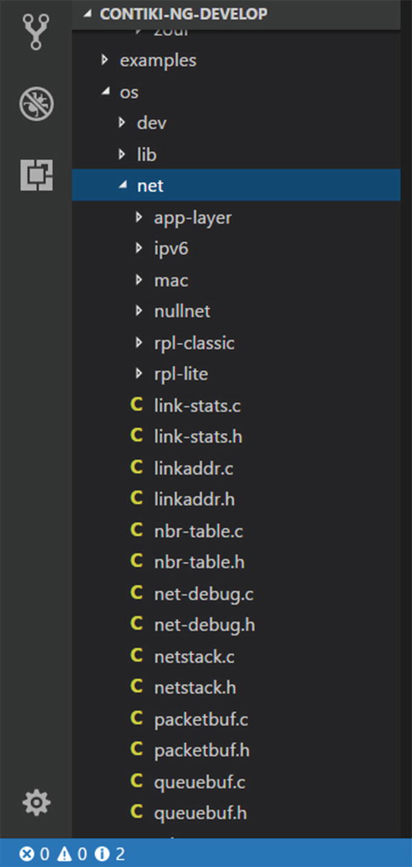
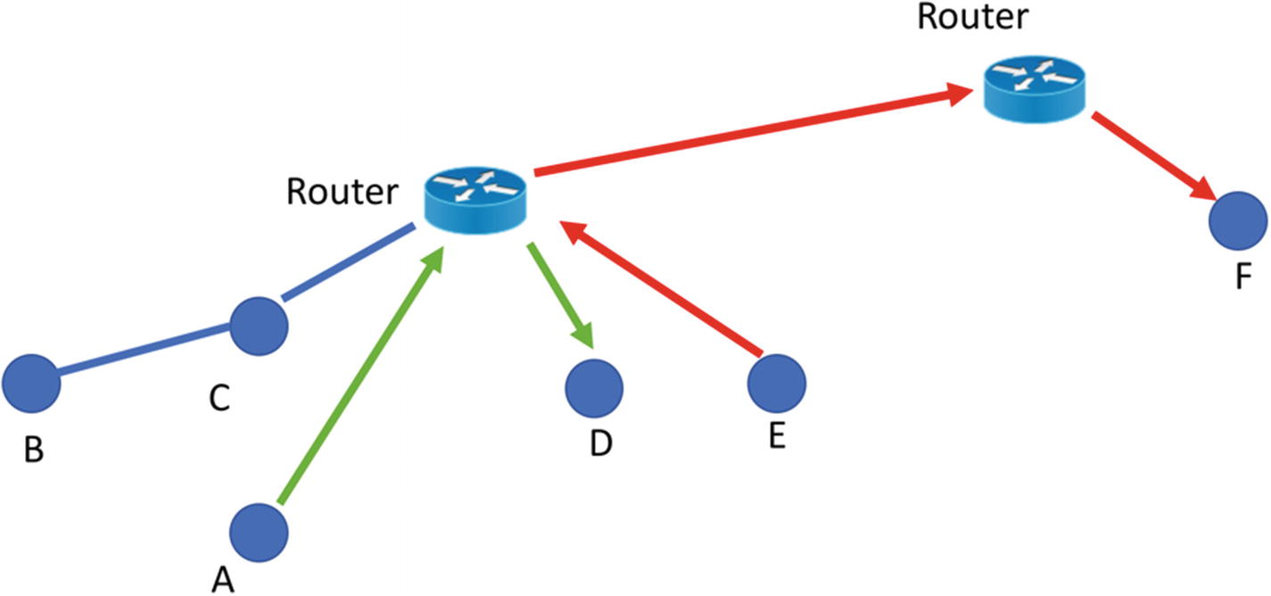
Data network flow on some motes
Figure 6-23 shows a number of path options to send a packet from A to D. We can take one of three path options: A-B-D, A-D, and A-C-D. Which one is the best path? This is a challenge.
When selecting a path, you must consider what your goal is and what your success criteria are. We can define a cost for each path. Then, we can select the best path with the lowest cost. Battery usage can be one of the cost parameters when you want to perform a certain routing algorithm.
That is one routing issue. Unfortunately, this book does not focus on routing algorithms. I recommend you read about routing topics in textbooks or technical articles. We will use the current routing algorithms that are applied in Contiki-NG.
Single-Hop and Multi-Hop Networking
When a packet is transferred from the source to the final destination, it probably goes through a number of network devices. In networking, we will find a term called a hop. Hop is a term used to describe the different network devices a packet has to go through to reach its final destination point.
We can categorize networking models by the number of hops, such as single-hop and multi-hop networks. To better understand these network models, see the network topology depicted in Figure 6-24. A single-hop network would be pointed to the A-D path. The packet is sent from A to D through a single router.
A network topology
The Contiki-NG platform supports both single-hop and multi-hop networks. Depending on your network design, your Contiki-NG program should be aware of single-hop and multi-hop networks.
Routing on Contiki-NG
Currently, Contiki-NG supports two RPL routing methods: RPL classic and RPL lite. RPL classic is the original Contiki’s RPL implementation, called ContikiRPL. If you want to read further about ContikiRPL, I recommend you read this paper: http://www.diva-portal.org/smash/get/diva2:1042739/FULLTEXT01.pdf . Otherwise, Contiki-NG applies RPL lite for default RPL implementation.
Since Contiki-NG applies RPL lite by default, we test RPL. For instance, we have two motes for testing. Enable NG shell on your program. You can use the hello-world program with NG shell enabled. Flash this program to all motes.
Now you can access the Contiki-NG motes via NG shell. First, test an RPL root on the first mote. You can type this command:
Then, you can check the RPL status using this command:
You also can check the RPL route table that is applied on this mote. Type this command:
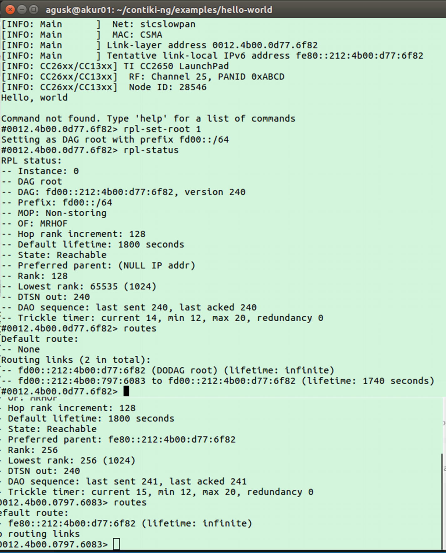
RPL operations on the first mote
Next, you also can check the RPL status and its routes on another mote. You can type these commands in the NG shell:
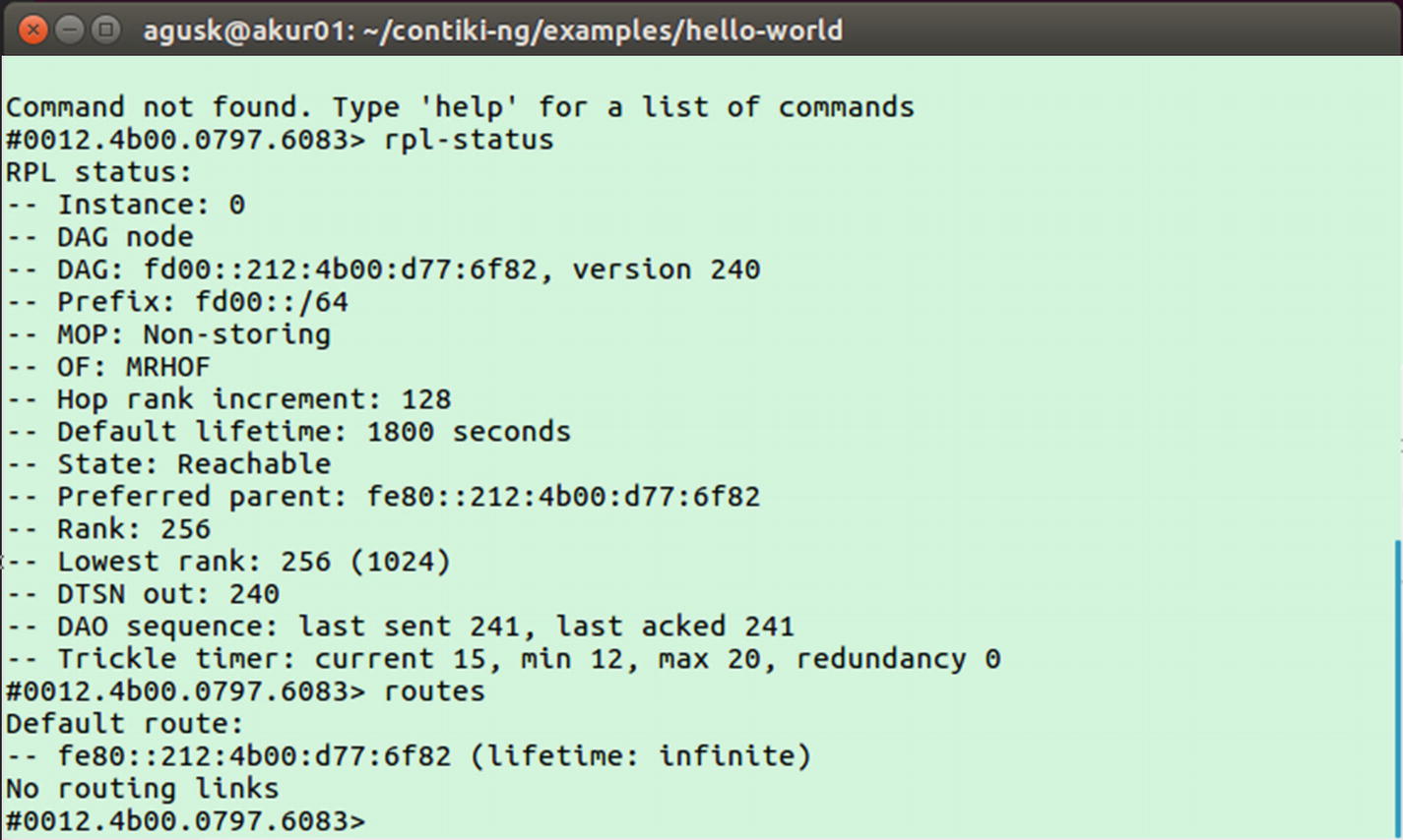
RPL operations on the second mote
IPv6 Multicast
We can categorize data communication based on how the data is transferred. There are three models in data communication: unicast, broadcast, and multicast.
Unicast describes communication where a piece of information is sent from one point to another point. In the Unicast model, there is one sender and one receiver. Network protocols–based TCP transport such as http, smtp, ftp, and telnet support the unicast transfer mode.
Broadcast is a communication model where a piece of information is sent from one point to all other points. In this model, there is still one sender, but the information is sent to all connected receivers. There may be no receivers. ARP (Address Resolution Protocol) uses broadcast to send an address resolution query to all computers.
Multicast describes communication where a piece of information is sent from one or more points to a set of other points. In this model, there may be one or more senders. The information is distributed to a number of receivers.
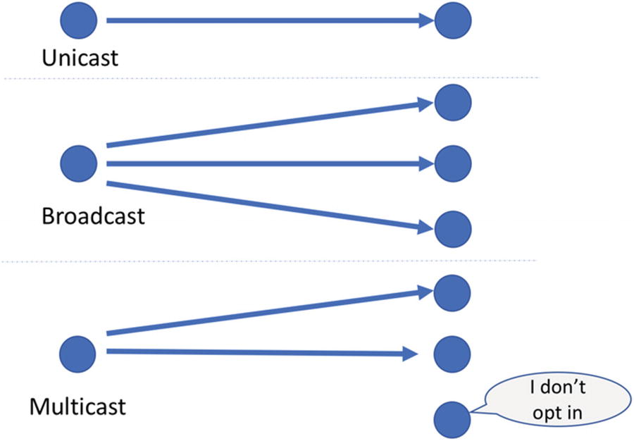
Unicast, broadcast, and multicast
To work with IPv6 multicast in a Contiki-NG project, you should add the multicast module to your project. You can add this script in the Makefile file:
We also activate RPL classic routing on the Contiki-NG project. You can add this script into the Makefile file:
For testing, we can use a program sample from Contiki-NG. We can use the multicast project from the <contiki-ng>/examples/multicast/ folder. For this demo, we need at least three motes. One mote is deployed for sink.c and another mote is deployed for root.c. The rest should be flashed for intermediate.c.
After deploying all programs to the motes, you can try to remote in to each mote. In general, the sink.c program will listen for incoming messages from root.c. Before listening for the message, the sink.c program should join the existing multicast group by calling the join_mcast_group() function. This program listens on port 3001:
The root.c program will send a UDP message every second. This is done by calling the uip_udp_packet_send() function. The intermediate.c program does not join the existing multicast group. Since the intermediate.c program has been activated for RPL classic routing, this program can forward any multicast message.
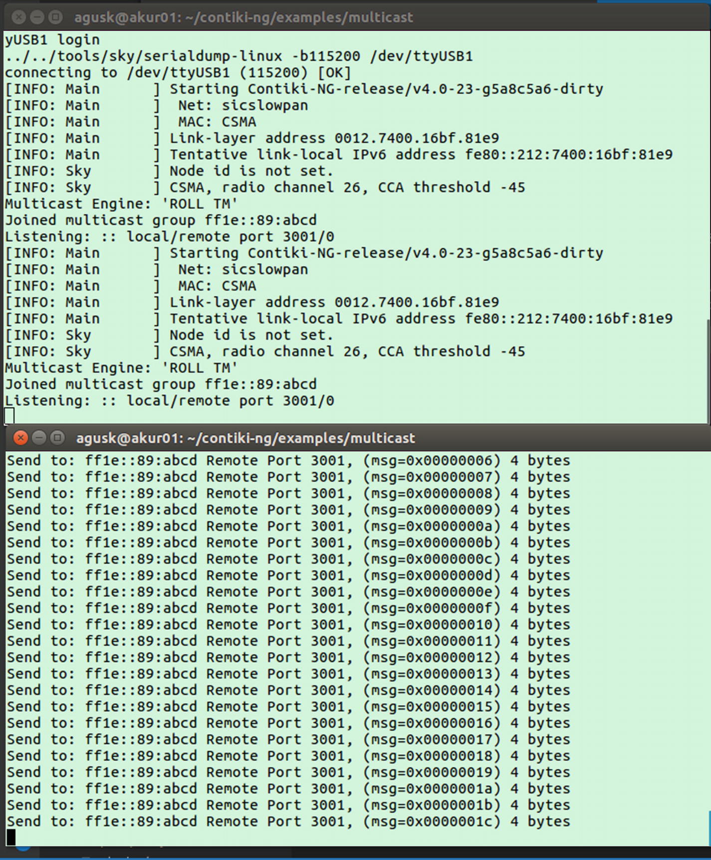
Multicast demo on Sky mote
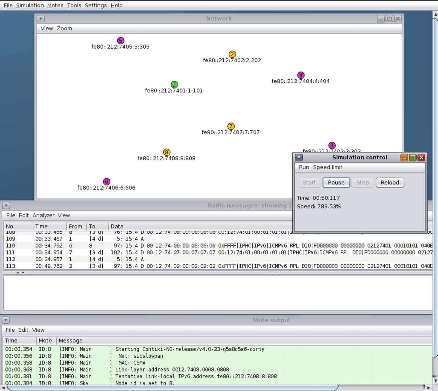
Multicast demo on COOJA tool
Contiki-NG NullNet
If you want to investigate a packet among Contiki-NG network stack layers, you can use NullNet. To work with NullNet, add this script to the Makefile file:
If you want to send data, you should the data and its size in the nullnet_buf and nullnet_len variables, which are pre-defined from net/nullnet/nullnet.h. Then, send the data by calling NETSTACK_NETWORK.output(NULL). To receive packets from NullNet, you call the nullnet_set_input_callback(callback_func) function with the passing callback function.
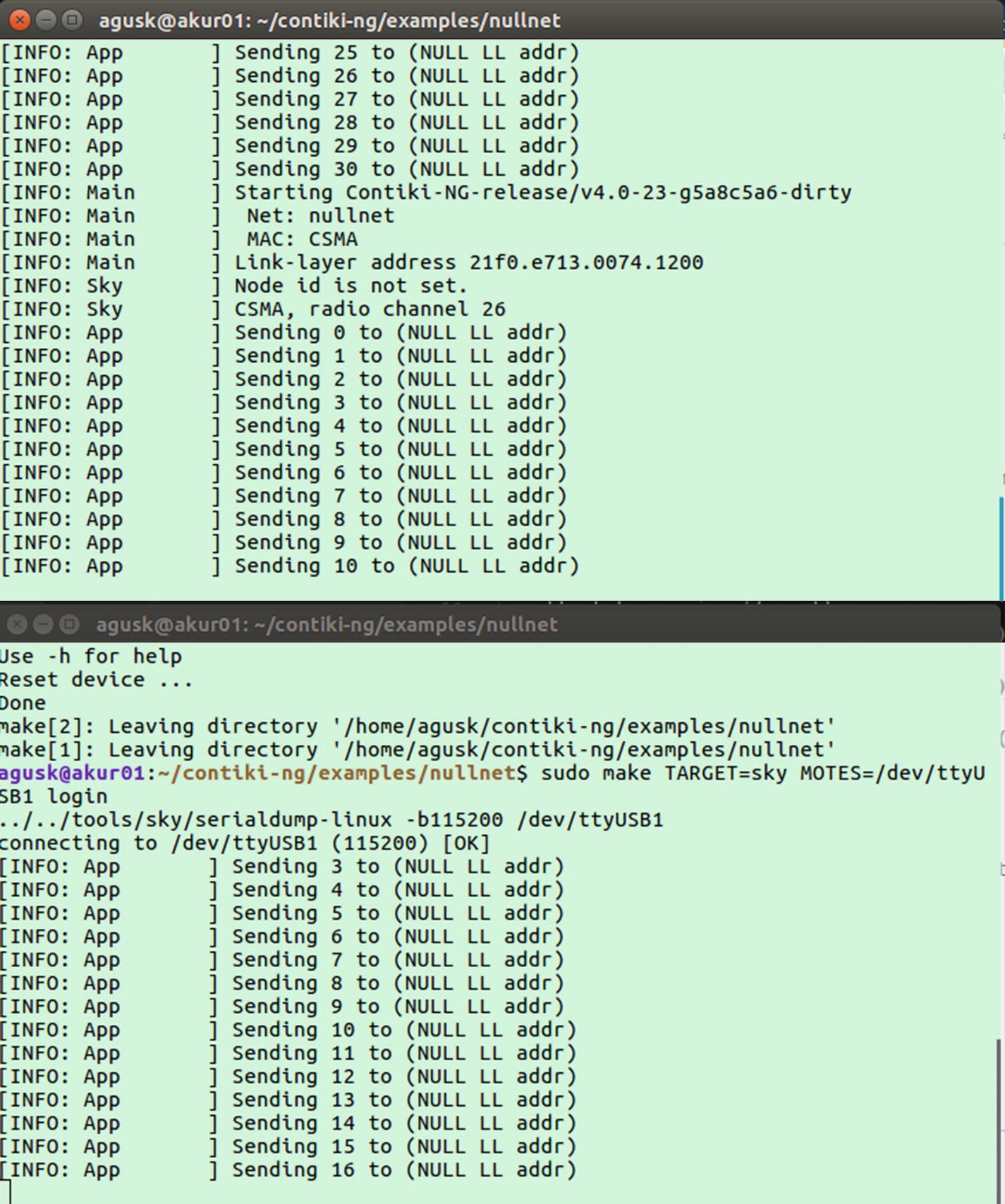
NullNet demo on Sky mote
You can also test this program demo using COOJA. Just select the nullnet-broadcast.csc and nullnet-unicast.csc files from the COOJA application. After they are loaded, you can run these demos and see radio messages from COOJA application and review pack flow.
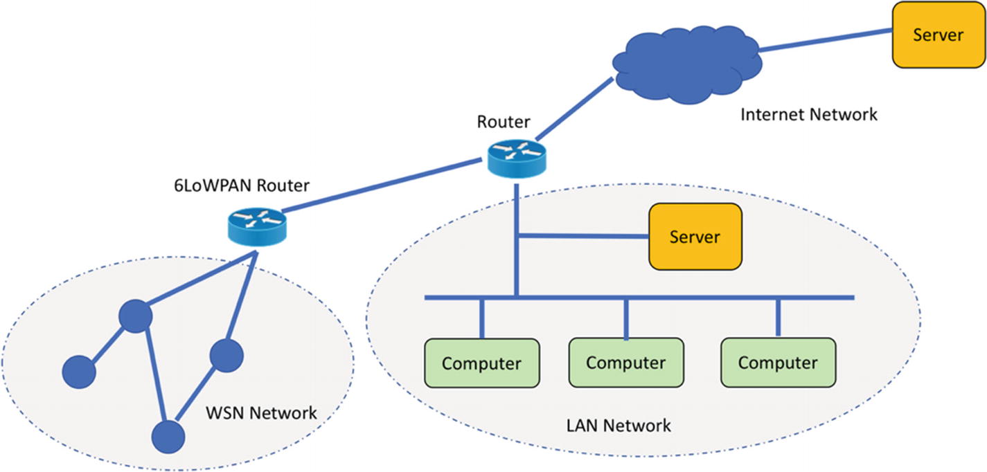
6LoWPAN Network
6LoWPAN is an acronym for IPv6 over Low-Power Wireless Personal Area Networks. 6LoWPAN is an open standard defined in RFC 6282. This standard enables WSN motes to communicate with other systems via an Internet network.
In this section, we will learn the basics of 6LoWPAN and how to implement it on the Contiki-NG platform.
A Brief Introduction
6LoWPAN network
WSN networks apply IPv6 for all communication. Each mote can communicate with the other motes. If one mote wants to communicate with an external system, such as a server, computer, or any legacy application in a different network, the mote just sends a message as usual. The 6LoWPAN router will take responsibility for communication between internal and external networks.
A 6LoWPAN router will record all addresses from motes and other network devices that are connected to the 6LoWPAN router. If an external system such as a server sends a message to one of the WSN motes in the WSN network, the 6LoWPAN router will forward the message to the mote. Otherwise, 6LoWPAN will inform the requester of failure.
In a network-stack view, we can compare a 6LoWPAN network to a WiFi network from the OSI layer side. You can see this comparison in Figure 6-32.
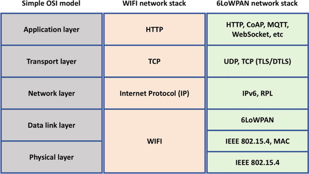
Comparing WiFi and 6LoWPAN to OSI model
In the next section, we will try to implement 6LoWPAN on Contiki-NG.
Implementing a 6LoWPAN Network on Contiki-NG
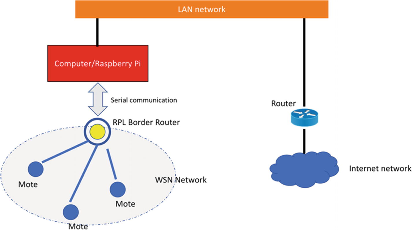
Contiki-NG implements the 6LoWPAN network stack via an RPL border router that acts as a 6LoWPAN router. You can see a network diagram in Figure 6-33 for implementing 6LoWPAN on the Contiki-NG platform. You can put the RPL border router on a computer or a Raspberry Pi or any network device.
How do you implement an RPL border router in Contiki-NG?
Basically, you need a Contiki-NG mote as the RPL border router mote. This mote will work as a bridge to serve all requests from motes in the WSN network or network devices from an external network. To create an RPL border router mote, you should add the rpl-border-router library into your project. You can add this script to your Makefile file:
Then, run a program, called tunslip6, from Contiki-NG. You can find it in the <contiki-ng>/tools/ folder. This tool will communicate with a mote that has already been deployed as an RPL border router via serial port. You can type this command:
Implementing 6LoWPAN network on Contiki-NG
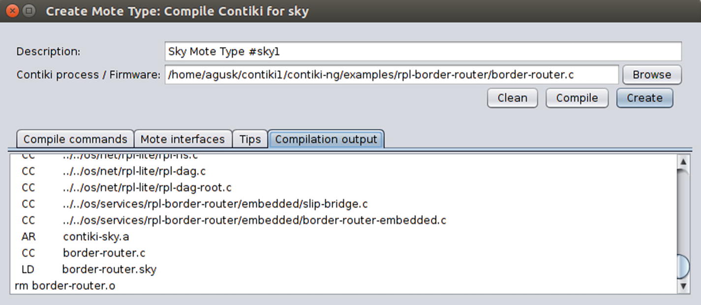
For this demo, we can run a program sample from the <contiki-ng>/examples/rpl-border-router/ folder. This project includes an RPL border router and web server modules. We need at least two motes to simulate the 6LoWPAN router and its communication.
Compile this project and flash it to one of the Contiki-NG motes. After it has been deployed to the mote, you can work remotely on the non–border router mote to see the assigned IPv6 address.
Last, you should run the tunslip6 program on the computer/Raspberry Pi to which the RPL border router mote was attached. You can run this command on the rpl-border-router project:
After being executed, that command will run tunslip6 with a default port. You should probably change the values for the target mote platform and its serial port.
By default, the RPL border router has an IPv6 address of fd00::1/64. You can change it in your Makefile. For instance, if you define the prefix of your IPv6 address as fd00::1/64, all motes within the WSN network will be assigned as fd00::xxxx. In this demo, my mote is assigned as fd00::212::4b00::d77::6fd2.
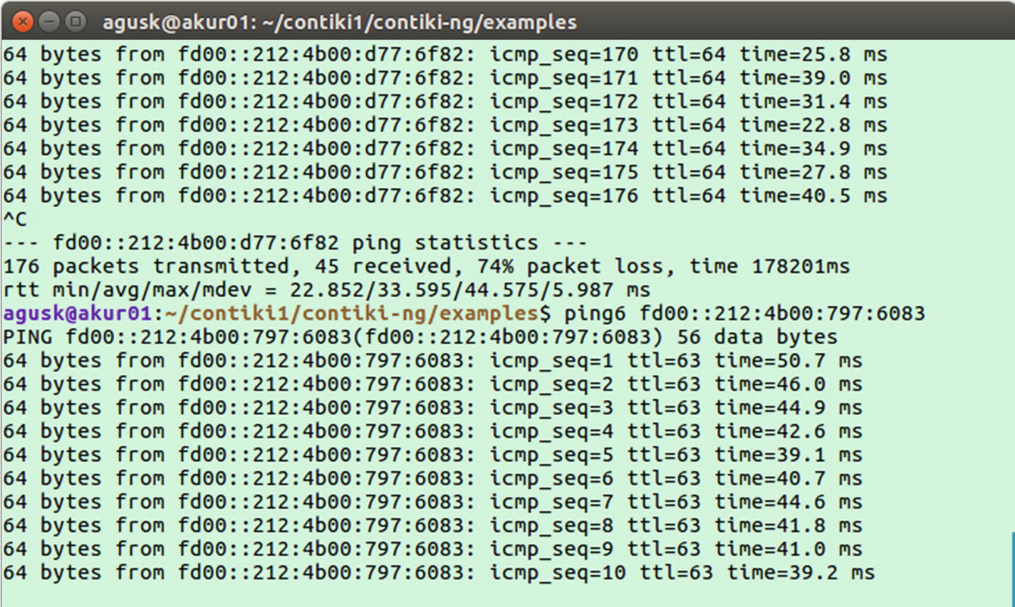
Now you can ping the mote using the assigned IPv6 address from your computer. For instance, type this command:
This program will get a response from the target mote because this mote can communicate with the computer through the RPL border router. You can see the program output in Figure 6-34. I ping my mote from Linux Ubuntu. It shows my computer can contact the Contiki-NG mote.
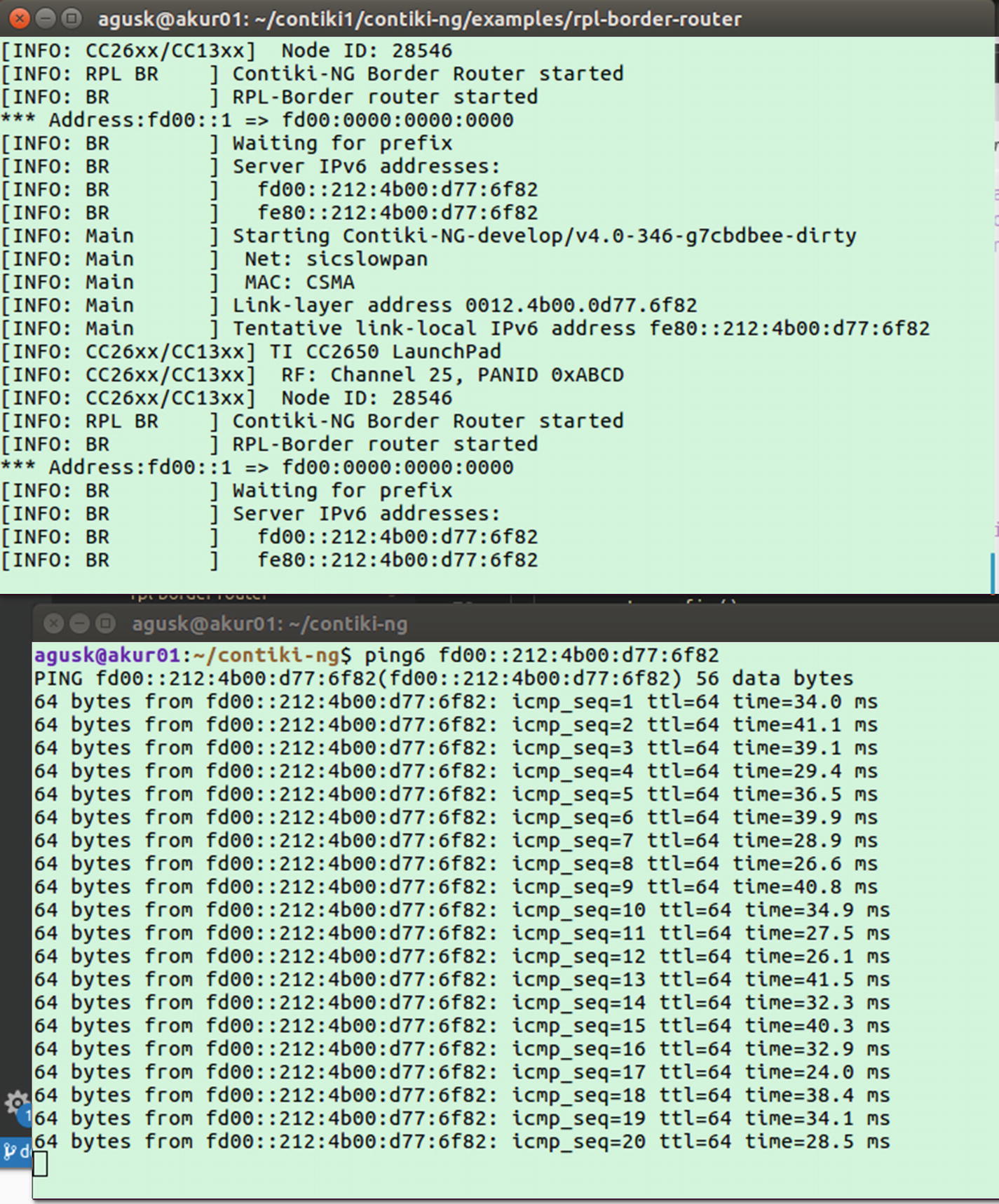
Performing ping on one of the Contiki-NG motes from a computer
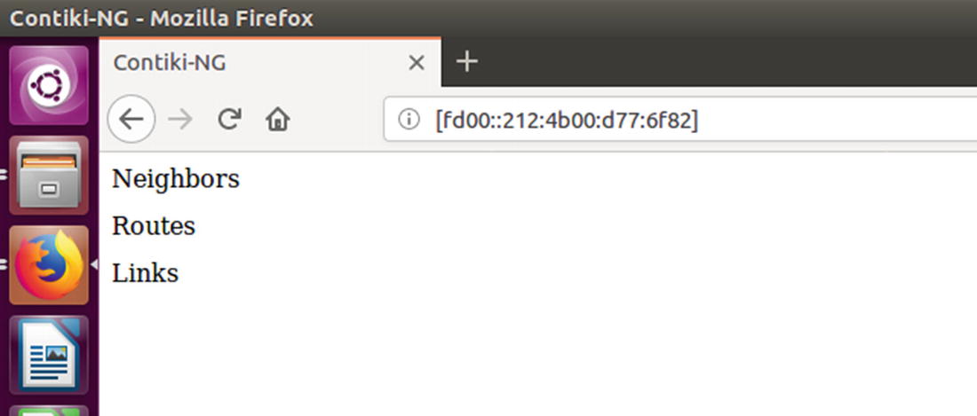
Accessing web server on Contiki-NG mote from computer browser
Displaying mote neighbor on RPL border router
You can also test it by performing a ping. For instance, the target mote is fd00::212:4b00:6083. We can perform a ping as follows:
You should get a response from that mote. You can see it in Figure 6-37.
Sometimes you don’t see the IPv6 address from a new mote in your browser (Figure 6-36), but you know the local IPv6 address of the new mote. You can verify it by remoting into the mote with the local IPv6 address. For instance, the IPv6 address is fe80::212:4b00:6083. Now, change the prefix to fd00::xxx. The new IPv6 address shows fd00::212:4b00:6083. Try to ping it.
Performing ping on other mote in WSN network from computer
6LoWPAN Implementation using COOJA
In the previous section, we learned how to implement 6LoWPAN on a physical device from a Contiki-NG mote. In this section, we want to implement 6LoWPAN on a simulation platform through the COOJA tool.
For this demo, we will use the program sample from the <contiki-ng>/examples/rpl-border-router/ folder. First, you can run the COOJA application. Create a new simulation project.
Add RPL border router into COOJA
You can compile this Contiki firmware. If there is no error, you can click the Create button. In this demo, you will create one mote.
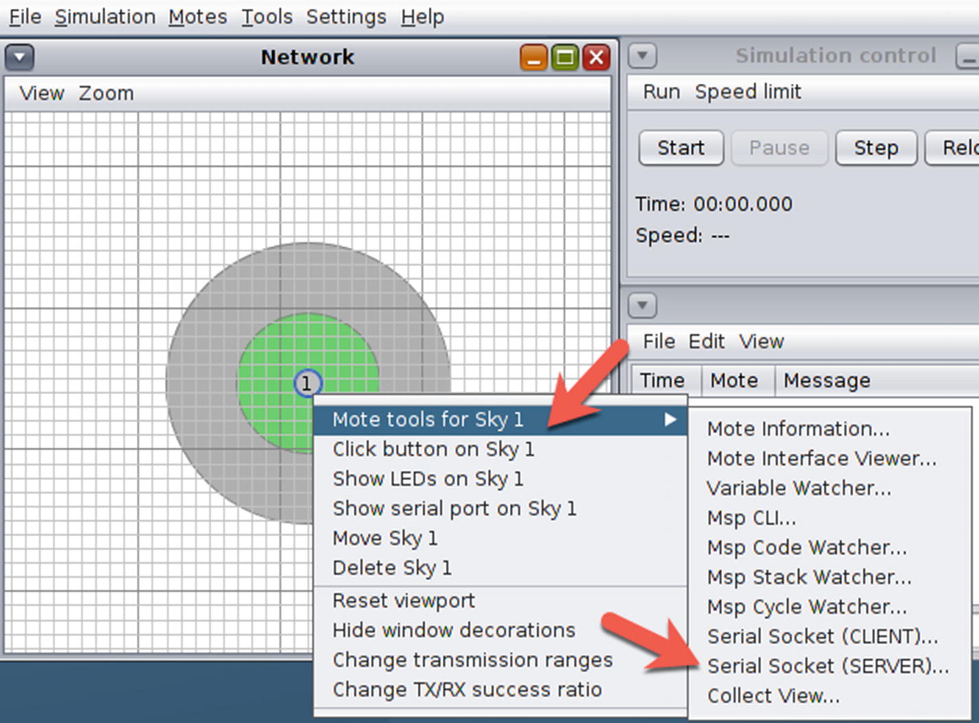
Add serial socket tool on RPL border router mote
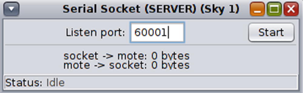
A serial socket dialog to set a listen port
Next, you should run tunslip6 from the <contiki-ng>/tools/ folder. You can open Terminal and navigate to <contiki-ng>/tools/. Then, you can run this command:
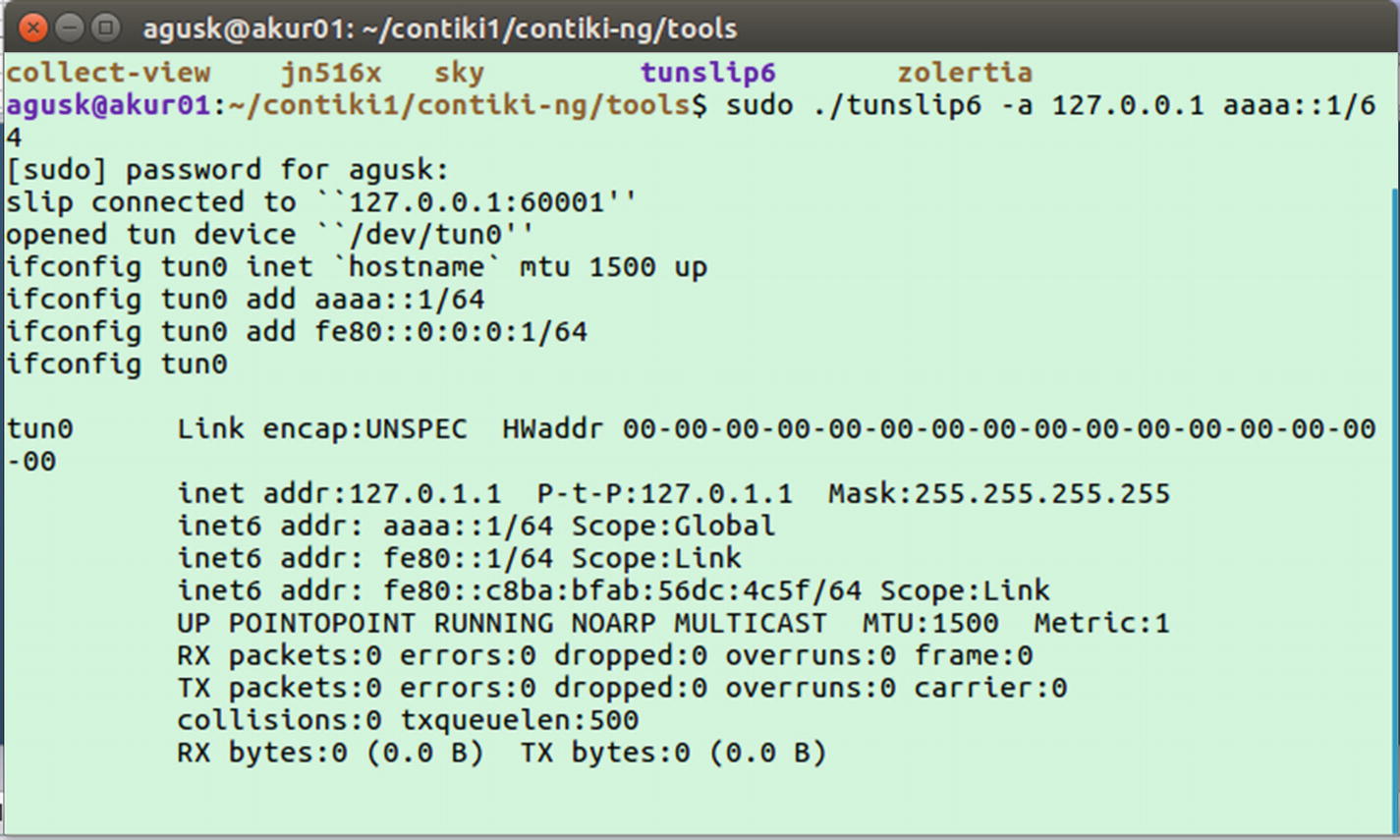
Running tunslip6 program on local computer
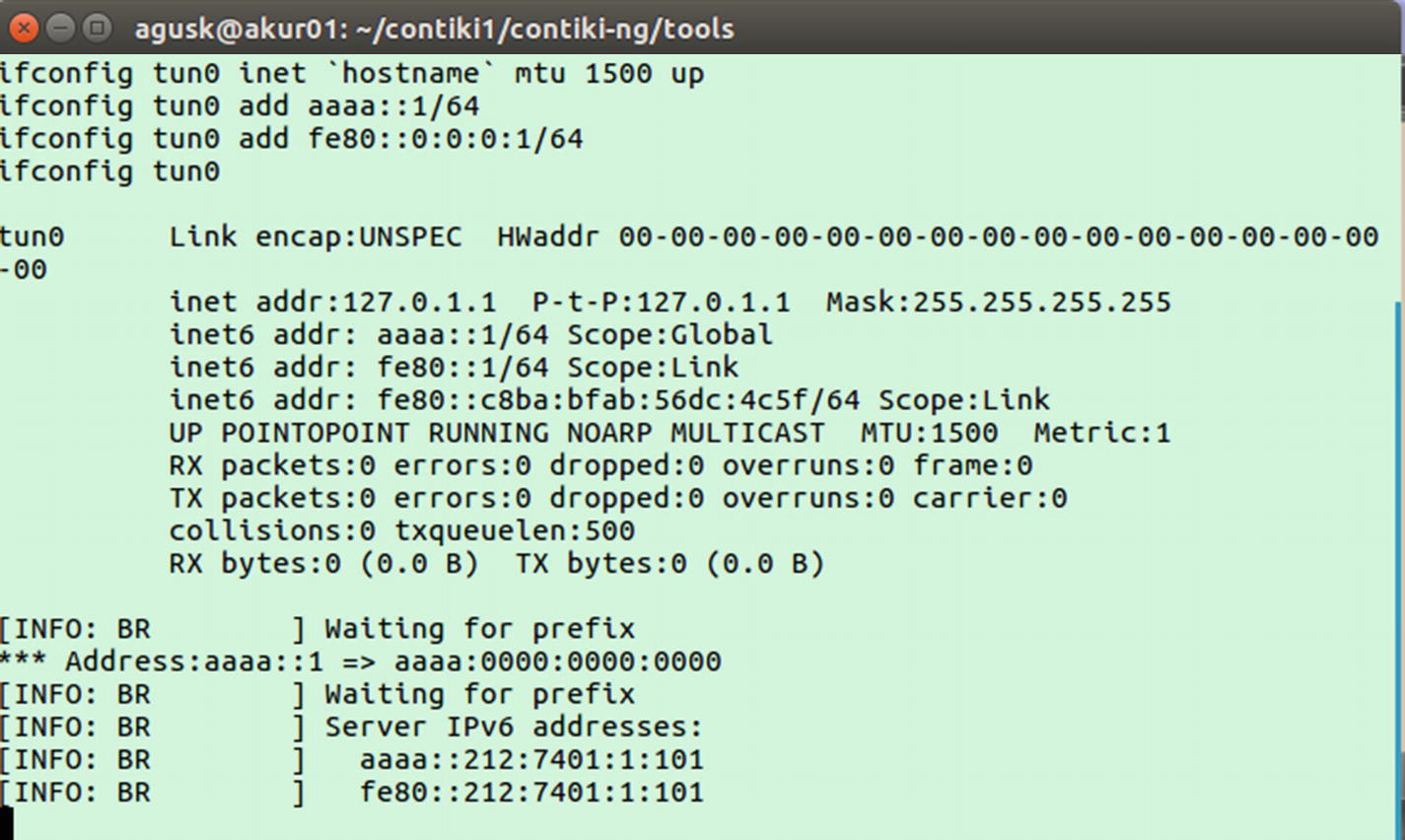
Detecting IPv6 address on tunslip6 tool
You should see the IPv6 address of the COOJA mote in Terminal. For instance, my mote IPv6 address is aaaa::212:7401:1:101. Now, you can open a new Terminal. Then, try to perform ping6.
You can type this command:
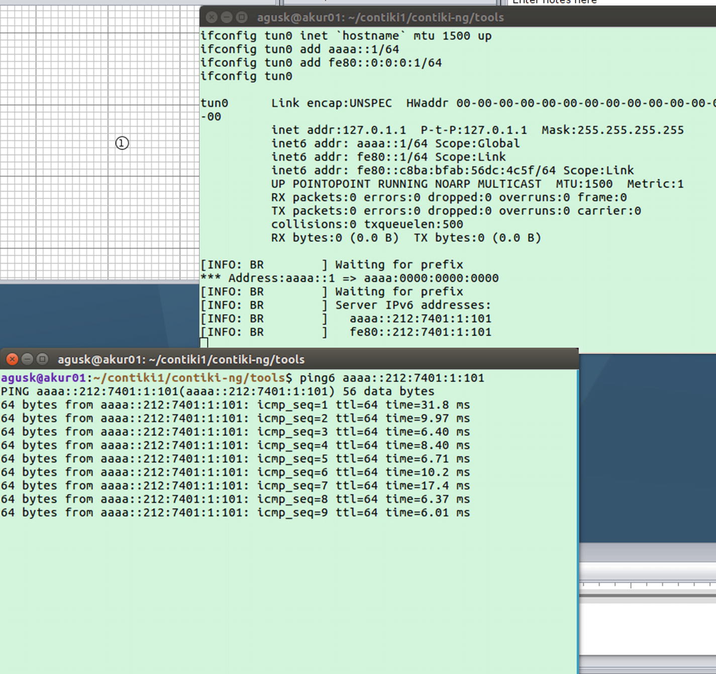
Pinging a mote from computer
To get more practice, you can run a web server program on a new mote in COOJA. Then, you can access that web server from a browser on a local computer.
Build Your Own RESTful Server for Contiki-NG
You have learned how to build a 6LoWPAN with RPL border router. In this section, we will build a simple project based on 6LoWPAN. We will develop WebSense, which publishes sensor values to the web server. Since a Contiki-NG mote has limited resources, it cannot serve many requests. To address this issue, we can implement a middleware server—for instance, a RESTful server.
Each mote will send a result of sensing to the RESTful server. Then, the RESTful server will take over to distribute the data to all requesters. A RESTful server can run on top of a proven web server, such as Apache, nginx, and IIS.
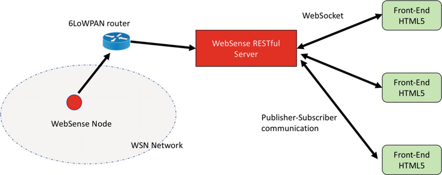
Logic design for the WebSense project
A client system will be implemented using HTML5 with WebSocket API. Sensor data will be visualized in the HTML5 application. Also, the WebSense RESTful server will apply Node.js.
We will implement this WebSense project in the next section.
Preparation
First, we should have two mote devices. One mote will be used for the 6LoWPAN router. The rest will be applied for WebSense node implementation.
Since our RESTful server uses Node.js, your computer should install Node.js runtime. You should install all required libraries to run Node.js. Type these commands:
We will use Node.js LTS version. For instance, I use Node.js LTS 6.x. You can install it by typing these commands:
The next step is to develop a program for the project. We will do so in the next section.
Implementing the Demo
We will implement the WebSense project as shown in Figure 6-45. It is a physical design from our demo. We deploy the RPL border router into one of the motes. This mote will be attached to a computer that will deploy Node.js too. This project will use real mote devices. You can also use COOJA for testing.
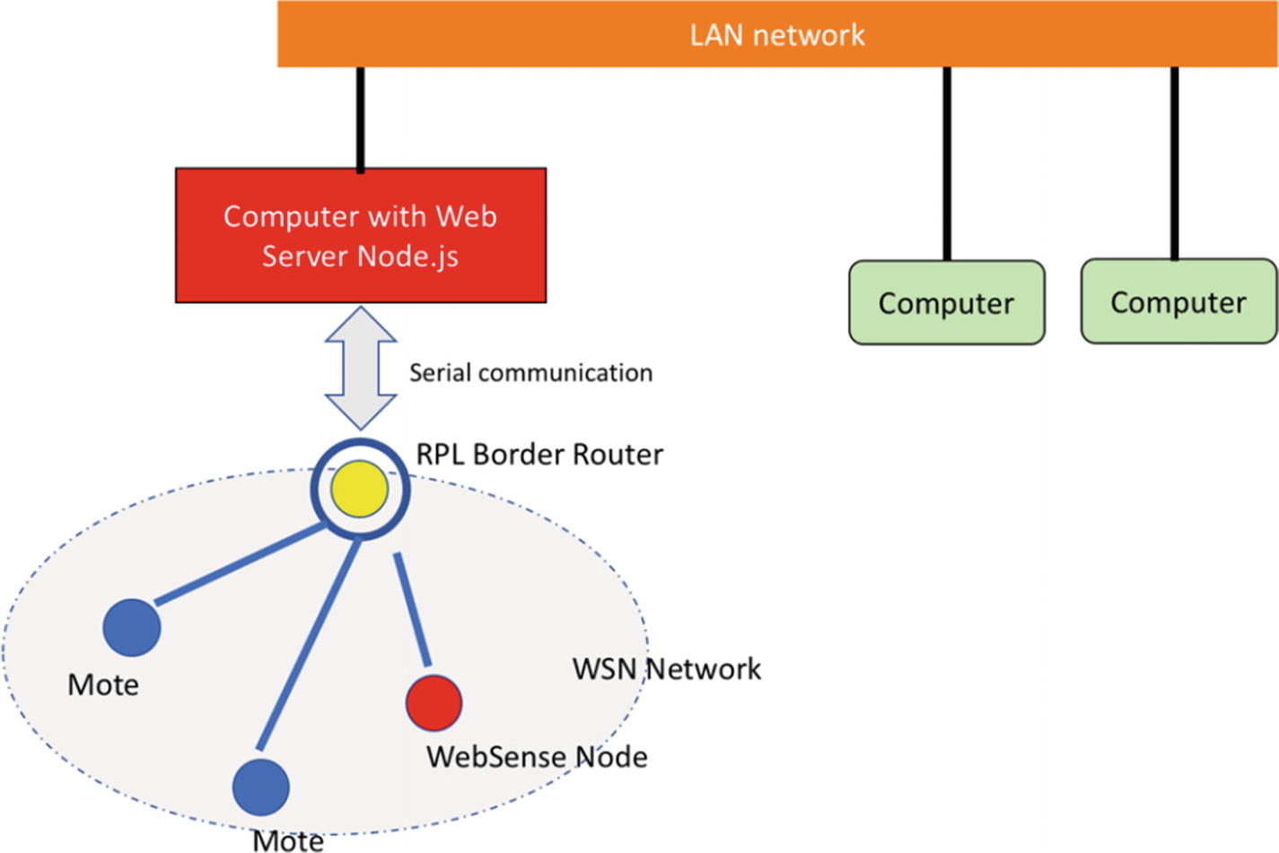
Implementing WebSense project
Implement 6LoWPAN router.
Develop a program for WebSense node.
Develop a program for RESTful server.
Test the project.
Each task will be presented in the following sections.
Implementing 6LoWPAN Router
To implement the 6LoWPAN router, we deploy the RPL border router module into the mote. In a previous section, you learned about 6LoWPAN router implementation. We will use it again in this project.
Select one of the motes to become a 6LoWPAN router. Attach it into a computer and run connect-router or run tunslip6 programs manually with specific port and address settings.
Writing a Program for WebSense Node
In this section, we will develop a program for the WebSense node. The goal of this program is to serve all requests for sensor data. Technically, the program will run a mini web server and serve HTTP requests. Once the RESTful server requests sensor data, this node will send it. To simplify this demo, the program will generate a random value for sensor data.
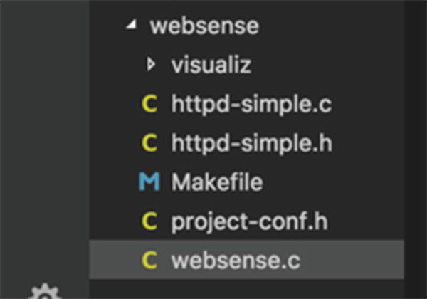
Project structure for WebSense node
The application will serve requests for sensor data. This task will be handled in websense.c in generate_routes() function. You can write this code as follows:
We also need to modify httpd-simple.c in order to cover JSON requests. We declare http_content_type_json for JSON content. Then, we pass it into the HTTP header as follows:
Writing a Program for RESTful Server
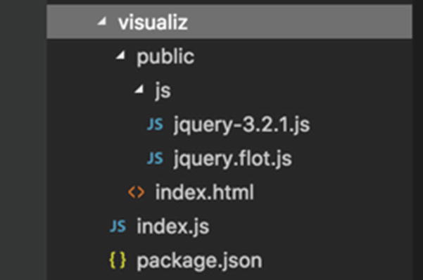
Project structure for RESTful server
The application runs with the Node.js runtime. Make sure you have already installed it. Next, we install required the libraries for the RESTful server. We will use Express ( http://expressjs.com ) for the web framework and Socket.io ( https://socket.io ) for WebSocket implementation for Node.js.
First, create a package.json file inside the project folder. You can type these scripts:
If done, save this file. Now, you can install all required libraries. You can type this command in the project folder. Make sure your computer is connected to the Internet:
Now you can write index.js for the application. This program will open a port 3000 to listen for HTTP requests. The program also requests sensor data from the WebSense node every three seconds. You can type these scripts for index.js:
You should change the IPv6 address of the WebSense node.
Next, we create index.html in the <project>/public folder. This program will communicate with the RESTful server though JSON communication. If the program receives sensor data, it will be stored into an array.
Then, the program will create a graphic for visualizing sensor data. You can type theses scripts for index.html:
Testing the Demo
Ensure the programs for the motes are already deployed. Now you can run the RESTful server by typing this command:
Accessing web server from RPL border router mote
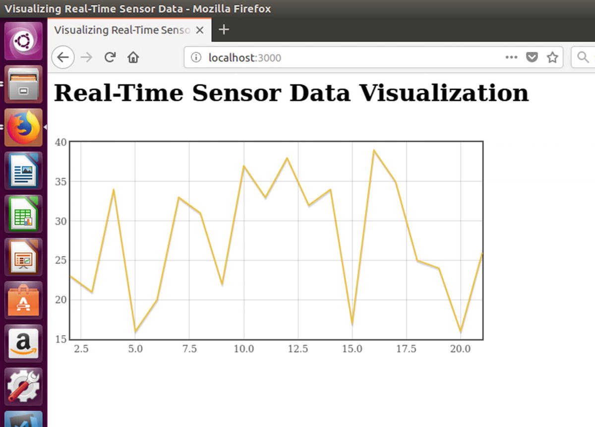
Accessing WebSense application using a browser
What’s next?
You can create more sensor sources in different sensor types from several motes. Then, you can modify sensor data visualization to cover multiple sensor types.
Summary
We have explored Contiki-NG networking. We have learned about routing models in Contiki-NG. Furthermore, we have worked with IPv6 multicast. We also implemented 6LoWPAN on physical motes and COOJA simulations. Last, we build sensor data visualization in real-time from a physical mote.
In the next chapter, we will learn to work with storage management in Contiki-NG.