
“If we have data, let’s look at data. If all we have are opinions, let’s go with mine.”
—Jim Barksdale, former CEO of Netscape
Big data strategy, as we learned, is a cost effective and analytics driven package of flexible, pluggable, and customized technology stacks. Organizations who embarked into Big Data world, realized that it’s not just a trend to follow but a journey to live. Big data offers an open ground of unprecedented challenges that demand logical and analytical exploitation of data-driven technologies. Early embracers who picked up their journeys with trivial solutions of data extraction and ingestion, accept the fact that conventional techniques were rather pro-relational and are not easy in the big data world. Traditional approaches of data storage, processing, and ingestion fall well short of their bandwidth to handle variety, disparity, and volume of data.
In the previous chapter, we had an introduction to a data lake architecture. It has three major layers namely data acquisition, data processing, and data consumption. The one that is responsible for building and growing the data lake is the data acquisition layer. Data acquisition lays the framework for data extraction from source data systems and orchestration of ingestion strategies into data lake. The ingestion framework plays a pivotal role in data lake ecosystem by devising data as an asset strategy and churning out enterprise value.
The focus of this chapter will revolve around data ingestion approaches in the real world. We start with ingestion principles and discuss design considerations in detail. The concentration of the chapter will be high on fundamentals and not on tutoring commercial products.
What is data ingestion?
Data ingestion framework captures data from multiple data sources and ingests it into big data lake. The framework securely connects to different sources, captures the changes, and replicates them in the data lake. The data ingestion framework keeps the data lake consistent with the data changes at the source systems; thus, making it a single station of enterprise data.
A standard ingestion framework consists of two components, namely, Data Collector and Data Integrator. While the data collector is responsible for collecting or pulling the data from a data source, the data integrator component takes care of ingesting the data into the data lake. Implementation and design of the data collector and integrator components can be flexible as per the big data technology stack.
Before we turn our discussion to ingestion challenges and principles, let us explore the operating modes of data ingestion. It can operate either in real-time or batch mode. By virtue of their names, real-time mode means that changes are applied to the data lake as soon as they happen, while a batched mode ingestion applies the changes in batches. However, it is important to note that real-time has its own share of lag between change event and application. For this reason, real-time can be fairly understood as near real-time. The factors that determine the ingestion operating mode are data change rate at source and volume of this change. Data change rate is a measure of changes occurring every hour.
For real-time ingestion mode , a change data capture (CDC) system is sufficient for the ingestion requirements. The change data capture framework reads the changes from transaction logs that are replicated in the data lake. Data latency between capture and integration phases is very minimal. Top software vendors like Oracle, HVR, Talend, Informatica, Pentaho, and IBM provide data integration tools that operate in real time.
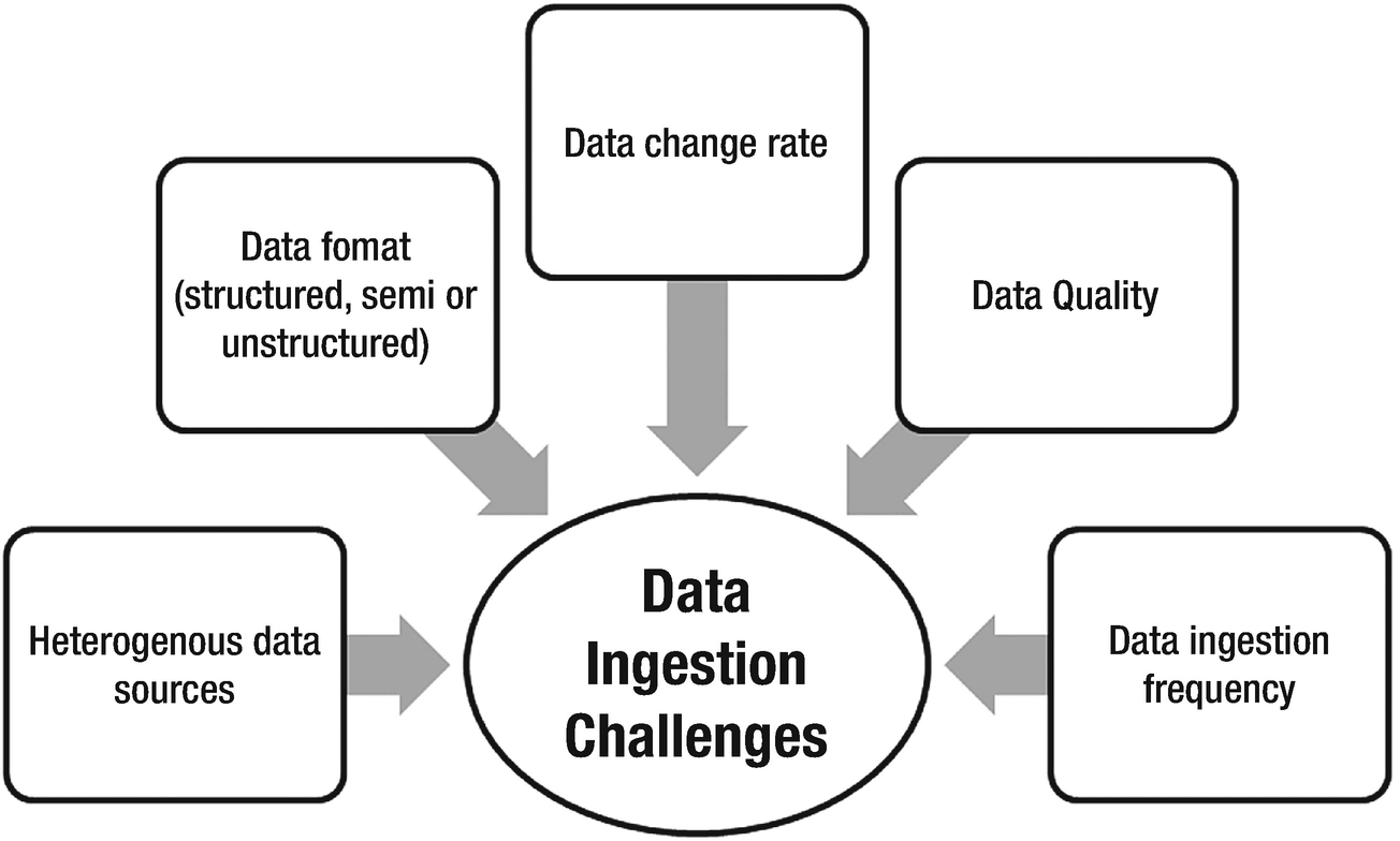
Data Ingestion challenges
Understand the data sources
OLTP systems and relational data stores – structured data from typical relational data stores can be ingested directly into a data lake.
Data management systems – documents and text files associated with a business entity. Most of the time, these are semi-structured and can be parsed to fit in a structured format.
Legacy systems – essential for historical and regulatory analytics. Mainframe based applications, customer relationship management (CRM) systems, and legacy ERPs can help in pattern analysis and building consumer profiles.
Sensors and IoT devices – devices installed on healthcare, home, and mobile appliances and large machines can upload logs to a data lake at periodic intervals or in a secure network region. Intelligent and real-time analytics can help in proactive recommendations, building health patterns, and surmising meteoric activities and climatic forecast.
Web content – social media platforms like Facebook, Twitter, LinkedIn, Instagram, and blogs accumulate humongous amounts of data. It may contain free text, images, or videos that is used to study user’s behavior, business focused profiles, content, and campaigns.
Geographical details – data flowing from location data, maps, and geo-positioning systems.
Structured vs. Semi-structured vs. Unstructured data
Data serves as the primitive unit of information. At a high level, data flows from distinct source systems to a data lake, goes through a processing layer, and augments an analytical insight. This might sound quite smooth but what needs to be factored in is the data format. Data classification is a critical component of the ingestion framework. Data can be either structured, semi-structured, or unstructured. Depending on the structure of data, the processing framework can be designed effectively.
Structured data is an organized piece of information that aligns strongly with the relational standards. It can be searched using a structured query language and the result containing the data set can be retrieved. For example, relational databases predominantly hold structured data. The fact that structured data constitutes a very small chunk of global data cannot be denied. There is lot of information that cannot be captured in a structured format.
Unstructured data is the unmalleable format of data. It lacks a structure; thus, making basic data operations like fetch, search, and result consolidation quite tedious. Data sourced from complex source systems like web logs, multimedia files, images, emails, and documents are unstructured. In a data lake ecosystem, unstructured data forms a pool that must be wisely exploited to achieve analytic competency. Challenges come with the structure and volume. Documents in character format (text, csv, word, XML) are considered as semi-structured as they follow a discernable pattern and possess the ability to be parsed and stored in the database. Images, emails, weblogs, data feeds, sensors, and machine-generated data from IoT devices, audio, or video files exist in binary format and it is not possible for structured semantics to parse this information.
“Unstructured information represents the largest, most current, and fastest growing source of knowledge available to businesses and governments. It includes documents found on the web, plus an estimated 80% of the information generated by enterprises around the world.” - Organization for the Advancement of Structured Information Standard (OASIS) - a global nonprofit consortium that works towards building up the standards for various technology tracks ( https://www.oasis-open.org/ ).

Unstructured data complexities
- 1.
Distributed storage and distributed computing – Hadoop’s distributed framework favors storage and processing of enormous volumes of unstructured data.
- 2.
Schema on read – Hadoop doesn’t require a schema on write for unstructured data. It is only post processing that analyzed data needs a schema on read.
- 3.
Complex processing – Hadoop empowers the developer community to program complex algorithms for unstructured data analysis and leverages the power of distributed computing.
Data ingestion framework parameters
Batch, real-time, or orchestrated – Depending on the transfer data size, ingestion mode can be batch or real time. Under batch mode, data movement will trigger only after a batch of definite size is ready. If the data change rate is defined and controllable (such that latency is not impacted), real-time mode can be chosen. For incremental change to apply, ingestion jobs can be orchestrated at periodic intervals.
Deployment model (cloud or on-premise) – data lake can be hosted on-premise as well as public cloud infrastructures. In recent times, due to the growing cost of computing and storage systems, enterprises have started evaluating cloud setup options. With a cloud hosted data lake, total cost of ownership (TCO) decreases substantially while return on investment (ROI) increases.
Data lineage – it is a worthwhile exercise to maintain a catalog of the source systems and understand its lineage starting from data generation until the ingestion entry point. This piece could be fully owned by the data governance council and may get reviewed from time to time to align and cover catalog registrants under the ongoing compliance regulations.
Data format – whether incoming data is in the form of data blocks or objects (semi or unstructured)
Performance and data change rate – data change rate is defined as the size of changes occur every hour. It helps in selecting the appropriate ingestion tool in the framework.
Performance is a derivative of throughput and latency.
- Data location and security
Whether data is located on-premise or in a public cloud infrastructure, network bandwidth plays an important role.
If the data source is enclosed within a security layer, the ingestion framework should be enabled and establishment of a secure tunnel to collect data for ingestion should occur.
Transfer data size (file compression and file splitting) – what would be the average and maximum size of block or object in a single ingestion operation?
Target file format – Data from a source system needs to be ingested in a Hadoop compatible file format.
File formats and their features
File type | Features | Usage |
|---|---|---|
Parquet | • Columnar data representation • Nested data structures | • Good query performance • Hive supports schema evolution • Optimized for Cloudera Impala • Slower write performance |
Avro | • Row format data representation • Nested data structures | • Stores metadata • Supports file splitting and block compression |
ORC | • Optimized Record Columnar files • Row format data representation as key-value pair • Hybrid of row and columnar format • Row format helps to keep data intact on the same node • Columnar format yields better compression | • Good for data query operations • Improved compression • Slow write performance • Schema evolution not supported • Not supported by Cloudera Impala |
SequenceFile | • Flat files as key-value pairs | • Limited schema evolution • Supports block compression • Used as interim files during MapReduce jobs |
CSV or Text file | • Regular semi-structured files | • Easy to be parsed • No support for block compression • Schema evolution not easy |
JSON | • Record structure stored as key-value pair | • No support for block compression • Schema evolution easier than CSV or text file as metadata stored along with data |
Why ORC is a preferred file format? ORC is a columnar storage format that supports optimal execution of a query through indexes which help in quick scanning of files. ORC supports indexes at the file level, stripe level, and row level. File and stripe indexes work similar to storage indexes from a relational perspective in that they help in quick scanning of data by narrowing down the scan surface area. They help in pruning out the stripes from scans during query execution.
- 1.
orc.compress – Compression codec for ORC file
- 2.
orc.compress.size – Size of a compression chunk
- 3.
orc.create.index – whether or not the indexes should be created?
- 4.
orc.stripe.size – Size of memory buffer (bytes) for writing
- 5.
orc.row.index.stride – Rows between index entries
- 6.
orc.bloom.filter.columns – BLOOM_FILTER stream created for each of the specified column
For more details on ORC parameter, you can refer to ORC Apache page – https://orc.apache.org/docs/hive-config.html.
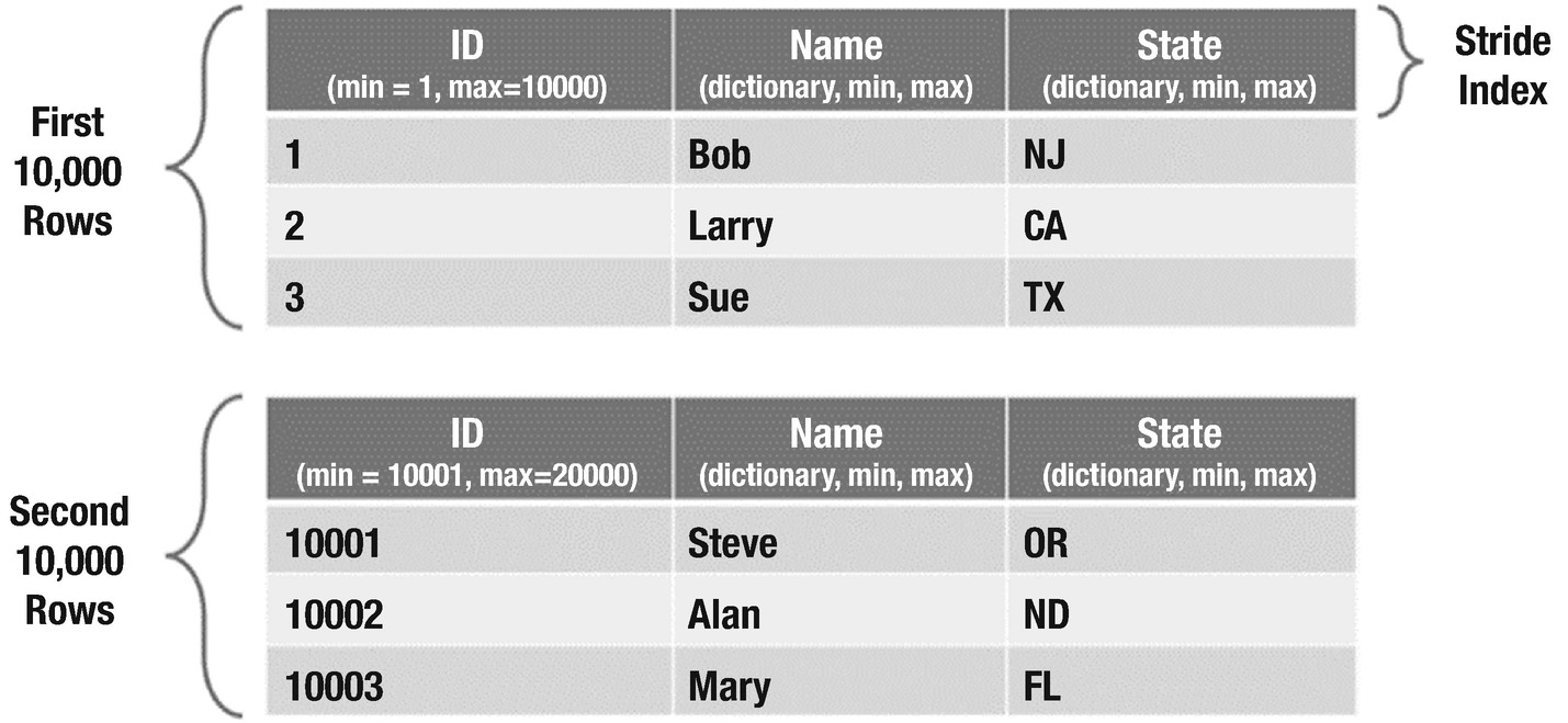
A user issues the below query. The query filters the results on “state” column.
For CUSTOMERS table, the two stripes have 10,000 rows each. The number of rows in a particular stripe is configurable while creating a table. Each stripe contains inline indexes such as min, max, and lookup/dictionary for the data within that stripe. ORC’s predicate pushdown will consult these inline indexes to identify if an entire block can be skipped all at once. The second stripe will be discarded because its index does not have the value “CA” in state column.
If a column is sorted, relevant records will get confined to one area on disk and the other pieces will be skipped very quickly. Skipping works for number types and for string types. In both instances, it’s done by recording a min and max value inside the inline index and determining if the lookup value falls outside that range. Sorting can lead to very nice speedups, but there is a trade-off with the resources needed in order to facilitate the sorting during insertion.
- 1.
Hive queries must be analyzed to explore usage patterns and track down columns that frequently occur in predicates.
- 2.
Hive tables must be timely analyzed to keep the statistics updated
- 3.
Data should be distributed and sorted during ingestion. This will help in effective resource management during query processing.
- 4.
If the filtering column in a query has high cardinality, then lower stripe size works well. If the cardinality is low, then a higher stripe size is preferred.
- 5.
Starting hive 1.2, support for bloom filters was included to ORC semantics to provide granular filtering. It is used on sorted columns.
The ORC file format is supported by Hive, Pig, Apache Nifi, Pig, Spark, and Presto. On the adoption fronts, Facebook and Yahoo use ORC file storage format in production and have observed significant performance compared to other formats.
ETL vs. ELT
It would be an understatement that Extraction, Transformation, and Loading (ETL) protocol under-sufficed the data motion requirements for traditional data warehouses. It has been a standard de-facto process since the evolution of data movement strategies. However, with the next-gen data warehousing strategies and big data trends, the ETL approach tends to require tweaks.
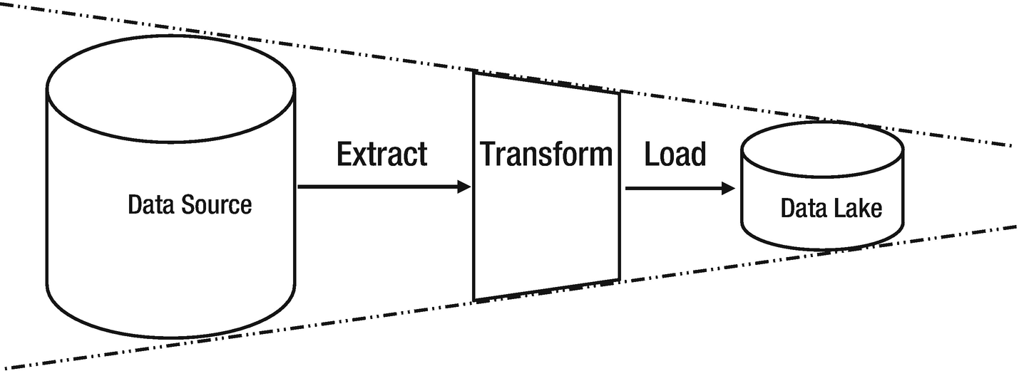
Data agility is reduced in a typical ETL process

Data agility remains intact in a typical ELT process
Other factors that stand in support of ELT in data lakes are cost effectiveness and maintenance. Since the time data lake concept has caught all the eyes of data world, ELT has been the most trusted approach.
Big Data Integration with Data Lake
Data is a ubiquitous entity. Until the big data trend acquired the waves, it was the relational databases who held the system of records in a structured format. Although relational data store vendors are finding ways to address unstructured data, adoption is majorly driven by factors like cost, ease of processing, and use-cases.
Data lakes are designed to complement contemporary data warehousing systems by empowering analytical models to churn out the real value of “data” irrespective of its format. In this chapter, we will cover techniques and best practices of bringing structured as well as unstructured data into data lake. This section focuses on bringing structured data into data lake. We will walkthrough ingestion concepts, best practices, and tools and technologies used in the process.
Hadoop Distributed File System (HDFS)
Although we assume the readers of this book to be proficient with Hadoop concepts and HDFS, but to maintain the logical flow of concepts, let us get a high-level overview of HDFS.
The Hadoop Distributed File System constitutes a layer of abstraction on top of POSIX (or like) file system. During a write operation, a file is split into small blocks and apparently replicated across the cluster. The replication happens transparently within the cluster while the replicas cannot be distinctly accessed. Replication ensures fault tolerance and resiliency. Whenever a file gets processed in the cluster, all its replicas are processed in parallel; thus, bettering the computational performance and scalability.
The hdfs dfs command-line utility can be used to issue the file system commands in the Hortonworks distribution of Hadoop. In addition to this utility, you can also use Hadoop’s web interface, WebHDFS REST API, or Hue to access the HDFS cluster.
- 1.
Shell commands are similar to common Linux file system commands such as ls, mkdir, cat
- 2.Help commands –
- a.
$ hdfs dfs
- b.
$ hdfs dfs -help
- c.
$ hdfs dfs -usage <shell command>
- a.
- 3.
Directory commands like cd and pwd not supported in HDFS.
Copy files directly into HDFS
One of the simplest methods to bring data into Hadoop is to copy the files from local to HDFS. If there are bunch of csv spreadsheets, JSON, or raw text files on the local system, you can copy the files directly into HDFS using put command.
Copies sales.csv from local to HDFS cluster
List the cluster files
Once the file is available in the Hadoop cluster, it can be consumed by Hadoop processing layers like hive data store, pig script, mapreduce custom programs or spark engine.
Batched data ingestion
In simple terms, batch is a frequency based incremental capture that kicks off as per the preset schedule . For most of the ETL frameworks, the implementation of the “extract” phase works on similar principles. Data collector fires a SELECT query (also known as filter query) on the source to pull incremental records or full extracts. Performance of the filter query determines how efficient a data collector is. The query-based approach to extract and load data is easy to implement with minimal failures.
- Change Track flag – if each changed record (insert/update/delete) on the source database can be flagged, the filter query can capture just the flagged records from the source table.
Primary key will be required to merge the changes at the target
- If primary key exists on target
Delete the existing record
Insert the fresh record from changed data set
- If primary key doesn’t exist on target
Insert the record from changed data set
If the target table is modeled as type 2 SCD (slowly changed dimension), all changed records can be directly inserted to target table. A timestamp attribute or transaction id can be maintained on target to trace change history of a primary key.
- Incremental extraction – the filter query pulls the differential data based on a column that can help in identifying changes in the source table. It can be a timestamp attribute or even a serialized id column.
To apply the changes, primary key is a must
If PK exists, delete old and insert the new record
If PK doesn’t exist, insert the new record
Incremental extraction frequency – from the data consistency perspective, it is important to be aware when the source table is active for transactions and what is data change rate. If the change rate is high, incremental job should be periodically orchestrated.
Full extraction – if the source database table is not very large and change frequency is low, target table can undergo full refresh every time the ETL runs. This ensures data consistency between source and target until source data gets modified. For source tables with master data and configuration data, full refresh approach can be followed.
Once captured from the source via filter query, the data extract needs to be staged on the edge node or ETL server, before its gets merged into Hadoop. This brings up the need for an additional storage system prior to the Hadoop cluster. The dual write approach adds to the latency and brings inconsistency in data lake.
Challenges and design considerations
An organizational data lake deals with all formats of data. Data, whether structured or unstructured, struggles with mutable data on Hadoop. Hadoop, being a distributed system relies on concurrency for functionality but dealing with mutability and concurrency could be meaty challenge. The ingestion framework must ensure that only one process updates the mutable object at a given time and avoids dirty read problems.
Other problems include datatype mismatch between source systems and hives, precision field handling, special character handling and efficient transfer of data with table size varying from Kilobyte (KB) to Terabyte (TB).
Design considerations
- 1.Table partitioning – Splitting the data into small manageable chunks provides better control in terms of resource consumption and data analysis. Partitioning strategy should factor in the following parameters –
- a.
Low-cardinality columns
- b.
Frequently used in joins and query predicates
- c.
Columns that can create interval based partitions
- a.
- 2.
File storage format – ORC file storage format gives better compression compared to other file formats. In addition, it also stores index headers for optimized read access from files.
- 3.
Full load or incremental - Full load integration should be practiced if change data capture is not possible. Data size and refresh frequency must be kept in mind while planning full load for objects.
- 4.
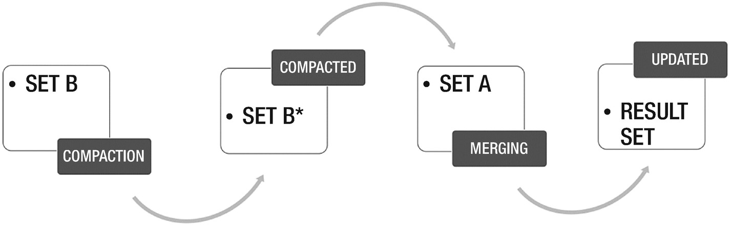
Change merge strategy – If the target landing table is partitioned, then the changes can be tagged by table and the most recent partition. During the exchange partition process, the recent partition can be compared against the “change” data set to merge the changes. Figure 2-5 shows the process flow of strategy to merge change using exchange partition for partitioned hive tables.

Merge changes through exchange partition
Let us consider a simple case of merging the changes using Piglatin. We have an interval partitioned hive table. The below code piece will show how to merge incremental changes from source data into a hive partition.
---sample data in a hive partition---
Changes are captured via a change capture tool. The changed data set has a delimiter “ctrl A”. Below is the change dataset that needs to be merged with most recent partition in hive table.
Pig script to merge the changes with original file.
Check and verify the changes in main file. Note that [id = 20001] has been deleted, [id=20003] has been updated, and [id=20015] has been inserted.
Let’s take another use case to demonstrate change-merge using Spark. We’ll work with a main data set and changed data set. Master Data in Target Location
Combining primary keys – pk1 AND pk2 … pkn
Combining primary keys having null – pk1 is null AND pk2 is null … pkn is null
P.K. | Name | VALUE | TIME_ID | DELETE_FLAG |
|---|---|---|---|---|
1 | Pranav | 13341 | 10001 | 0 |
2 | Shubham | 18929 | 10002 | 0 |
3 | Surya | 12931 | 10003 | 0 |
4 | Arun | 12313 | 10004 | 0 |
5 | Rita | 12930 | 10005 | 0 |
6 | Kiran | 12301 | 10006 | 0 |
7 | John | 82910 | 10007 | 0 |
8 | Niti | 218930 | 10008 | 0 |
9 | Sagar | 82910 | 10009 | 0 |
10 | Arjun | 92901 | 10010 | 0 |
P.K. | Name | VALUE | TIME_ID | DELETE_FLAG |
|---|---|---|---|---|
1 | Pranav | 13341 | 10020 | 1 |
2 | Shubham | 18929 | 10022 | 1 |
3 | Surya | 453202 | 10034 | 2 |
4 | Tarun | 489503 | 10098 | 0 |
5 | Pranav | 129789 | 10099 | 2 |
Here P.K. is the primary key column, TIME_ID is the defined value for timestamps and DELETE_FLAG is the value where 0 is termed as New Insert, 1 as Delete and 2 as an Update. The following spark code will merge the data and store it as a temporary view
Merge operation workflow process
P.K. | Name | VALUE | TIME_ID | DELETE_FLAG |
|---|---|---|---|---|
1 | Pranav | 129789 | 10099 | 0 |
3 | Surya | 453202 | 10034 | 0 |
4 | Arun | 12313 | 10035 | 0 |
5 | Rita | 12930 | 10036 | 0 |
6 | Kiran | 12301 | 10006 | 0 |
7 | John | 82910 | 10007 | 0 |
8 | Niti | 218930 | 10008 | 0 |
9 | Sagar | 82910 | 10009 | 0 |
10 | Arjun | 92901 | 10010 | 0 |
11 | Tarun | 489503 | 10098 | 0 |
Commercial ETL tools
While the underlying principle of most of the 3rd party commercial ETL tools remain as discussed above, implementations can be different. For example, Informatica PowerCenter stores metadata in an Oracle database repository while Talend generates java code to do the job. Pentaho, on the other hand, provides a user-friendly interface.
Because data lake is a new opportunity, data integration software vendors have started complementing their ETL products with Hadoop centric capabilities. Modern-day ETL tools are flexible, platform agnostic, and capable of optimized extraction, through reusable code generation, and much more.
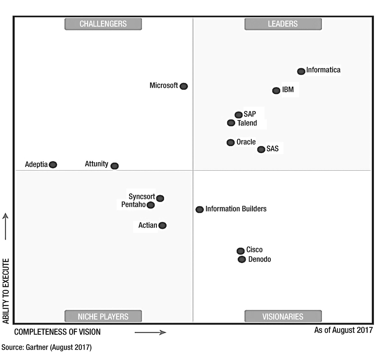
Gartner’s magic quadrant for commercial data integration products. https://www.informatica.com/in/data-integration-magic-quadrant.html
Real-time ingestion
A batched data ingestion technique is fool-proof as far as data sanity checks are concerned. However, it fails to paint the real-time picture of the business due to the lag associated with it. To enhance the business readiness of analytical frameworks, it is expedient to process a business transaction as soon as it occurs. In (near) real-time processing, changes are captured either at very low latency or in real-time. A log-based real-time processing exercise is known as change data capture.
Change data capture refers to the log mining process to capture only the changed data (insert, update, delete) from the data source transaction logs. A real-time or micro-batch CDC detects the change events by scanning the database logs as they occur. With minimal access to enterprise sources, CDC incurs no load on source tables; thereby minimizing latency and ensuring consistency between source and target systems.
So, why CDC? As we discussed in the last section, conventional ETL tools use SQL to extract and batch the incremental data. Query performance may be impacted due to continuous growth in source database’s volume and its concurrent workload. In addition, the query incurs its portion of the workload on the source system.
Change Data capture workflow
As part of business intelligence and data compliance initiatives, CDC helps in aligning with data-as-a-service principles by providing master data management capabilities and enabling quicker data quality checks.
Eliminating the need to run SQL queries on source system. Incurs no load overhead on a transactional source system.
Achieves near real-time replication between source and target
Log mining helps in capturing granular data operations like truncates as well
CDC design considerations
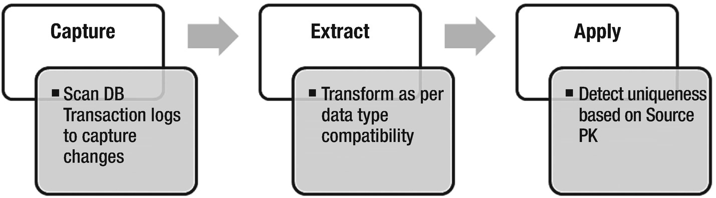
To design a CDC ingestion pipeline, the source database must be enabled for logging. All relational databases follow a roll forward approach by persisting the changes in logs. Each and every event is persistently logged with a change id (or system change number) in a log and will never get purged. An Oracle database allows enabling supplement logging at the table level. Similarly, SQL Server allows logging at the database level. Without logging, transaction logs cannot be mined to capture the changes.
The tables at the source database must hold a primary key for replication. It helps the capture job in establishing uniqueness of a record in the changed data set. A source PK ensures the changes are applied to the correct record on target. If the source table doesn’t have primary key defined, CDC job can designate a composite primary key to uniquely identify a record in the change table.
It would be a terrible design to establish uniqueness based on a unique constraint as it allows multiple NULLs in a column. In the apply phase, a change record with null identity will fail to pick a matching null record at the target.
Trigger based CDC –Another method of setting up change-data-capture is through triggers at the table level. A trigger helps in capturing row changes in a separate table synchronously, which apparently gets replicated to the target. Either the entire record is captured or just the changed attributes along with the primary key. The downside of this approach is that it induces overhead of one more transaction before the original transaction is deemed complete.
Logging not enabled on the source database
Reading transaction logs is a tedious task due to its binary format
T-logs not available for scanning due to software restriction or small retention time
So, should you always prefer CDC over batched ingestion? No. Real-time integration or CDC should be set up only when business demands it. It is a feature to be contemplated based on multiple factors like business’s service-level agreement, change size, and target readiness.
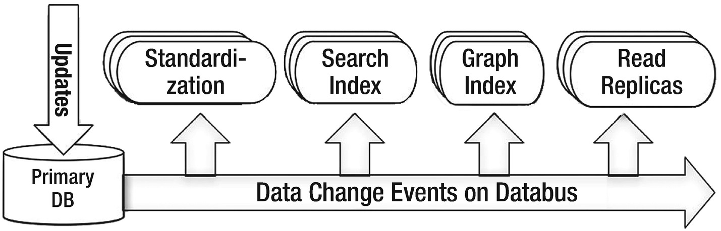
Example of CDC pipeline: Databus, LinkedIn’s open-source solution
Databus , a real-time change data capture system, was developed by LinkedIn in the year 2006. In 2013, LinkedIn released the open-source version of Databus. Since its development, Databus has been an essential component of the data processing framework at LinkedIn. Databus provides a real-time data replication mechanism with the ability to handle high throughput and latency in milliseconds. The Databus source code is available at its git repo at https://github.com/linkedin/databus .
Databus component diagram. Source: https://engineering.linkedin.com/data-replication/open-sourcing-databus-linkedins-low-latency-change-data-capture-system
- Relay is responsible for pulling the most recent committed transactions from the source
Relays are implemented through tungsten replicator
Relay stores the changes in logs or cache in compressed format
Consumer pulls the changes from relay
- Bootstrap component – a snapshot of data source on a temporary instance. It is consistent with the changes captured by Relay . (Refer to Figure 2-11)
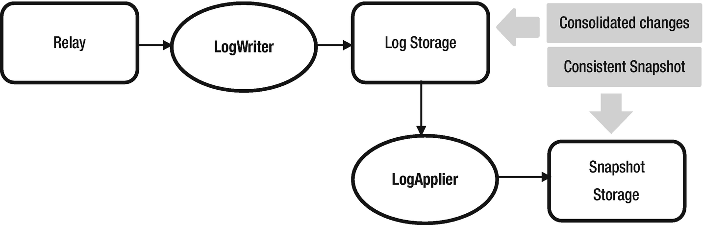 Figure 2-11
Bootstrap component in Databus
If any consumer falls behind and can’t find the changes in relay, bootstrap component transforms and packages the changes to the consumer
A new consumer, with the help of client library, can apply all the changes from bootstrap component until a time. Client library will point the consumer to Relay to continue pulling most recent changes
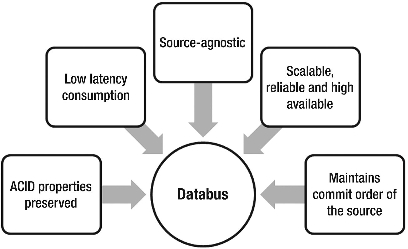
Linkedin’s Databus differentiators
Apache Sqoop
Sqoop or “SQL to Hadoop ” has been one of the top Apache projects that addresses the data integration requirements of Hadoop. It is a native component of the HDFS layer that allows bi-directional “batched” flow of data from the Hadoop distributed file system. Not just the users can automate data transfer between relational databases and Hadoop, but a reverse operation empowers enterprise data warehouses to augment their consumption layer with map-reduced data from data lake.
Apache Sqoop is available in two versions – sqoop 1 and sqoop 2.
Sqoop 1
The very first version of Sqoop was introduced in 2009. In August 2011, the project moved under Apache and quickly, Sqoop became one of the most sought-after ingestion tools.
Java based utility (web interface in Sqoop2) that spawns Map jobs from MapReduce engine to store data in HDFS
Provides full extract as well as incremental import mode support
Runs on HDFS cluster and can populate tables in Hive, HBase
Can establish a data integration layer between NoSQL and HDFS
Can be integrated with Oozie to schedule import/export tasks
Supports connectors to multiple relational databases like Oracle, SQL Server, MySQL
Sqoop 2
Sqoop2 succeeded sqoop with a major focus on optimizing data transfer, easing of using extension framework, and ensuring security. Sqoop2 works on client-server architecture (service-based model) in which the server acts as the host for two critical components, the connectors and the jobs.
Sqoop 2 can act as a generic data transfer service between any-to-any systems.
Sqoop 2 comes with a web interface for better interactivity. Command line utility still works. Sqoop 2 web interface uses REST services running on sqoop server. It helps in easy integration with Oozie and other frameworks.
Sqoop 2 employs both mapper and reducer jobs during data transfer activity. Mapper jobs extract the data, while the reducer operation transforms and loads the data into the target.
Connectors will be setup on Sqoop 2 server which requires connection details to the source and targets. Role-based access to connection objects mitigates the risk of unauthorized access on source and target systems.
The metadata repository stores connections and jobs. Connectors register metadata on the sqoop server to allow the connection to the source and the creation of jobs.
The connector consists of partitioning API (create splits and enabled parallelism), Extract API (Mappers), and Loading API (Reducers)
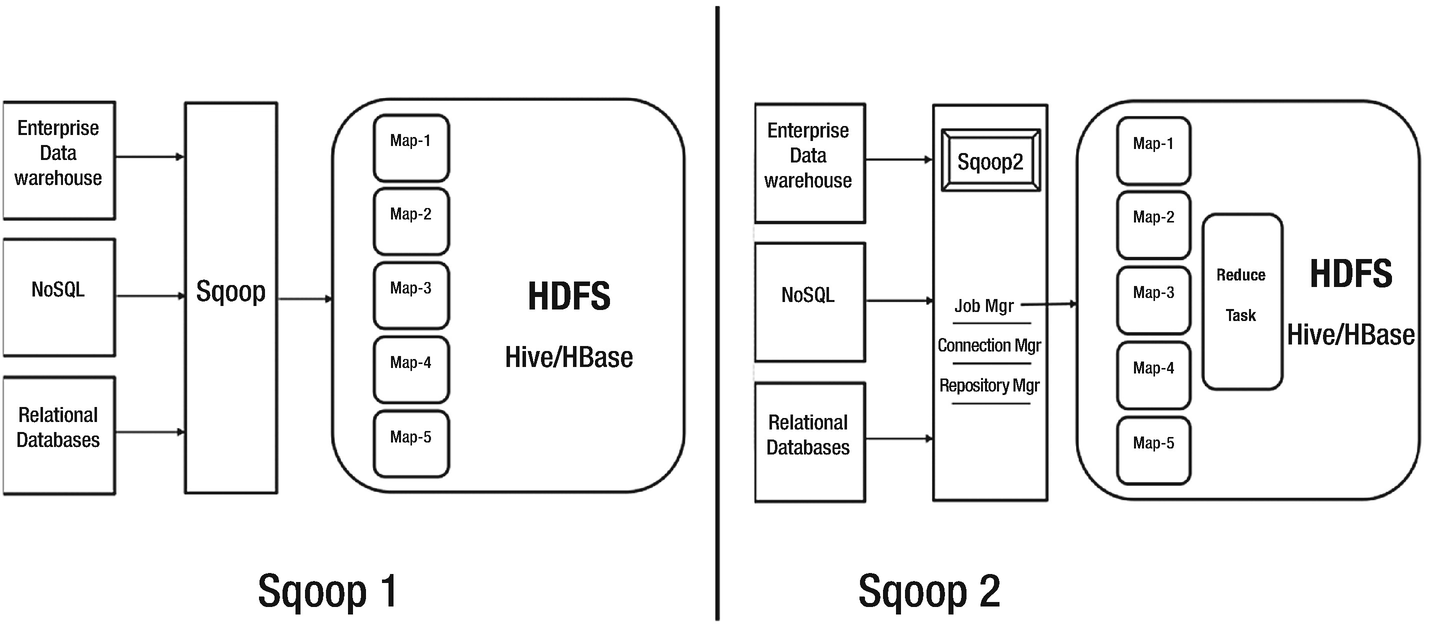
Sqoop 1 vs Sqoop2
How Sqoop works?
Sqoop adopts quite a simple approach to extract data from a relational database. In a nutshell, it builds up an SQL query that runs at the source to capture the source data, which later gets ingested into Hadoop. Let us look at the internals of Sqoop.
Sqoop leverages mapper jobs of MapReduce processing layer in Hadoop, to extract and ingest data into HDFS. By default, a sqoop job has four mappers; this number is configurable though. Each of these mappers is given a query to extract data from the source system. Query for a mapper is build using a split rule. As per the split rule, the values of --split-by column must be equally distributed to each mapper. This implies that --split-by column should be a primary key. The entire range of PK is equally sliced for the mappers. Once the mapper jobs capture source data, either it is dumped in HDFS storage or loaded into hive tables.
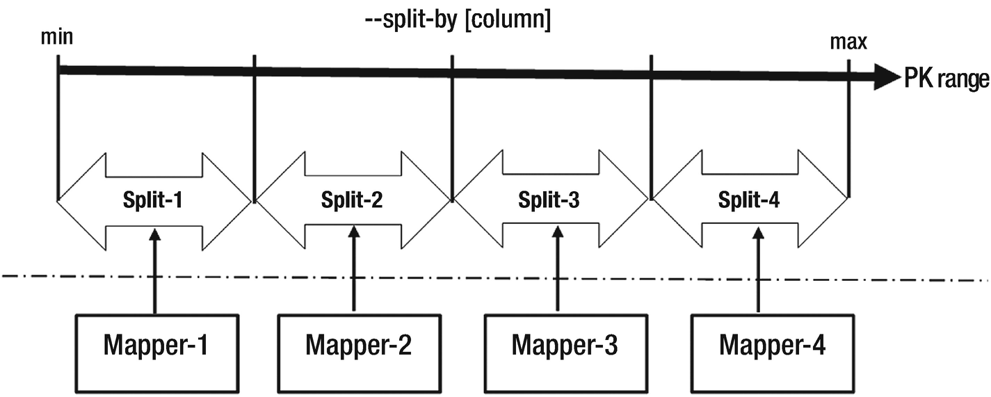
Sqoop split mechanism
Sqoop design considerations
- 1.
Specify number of mappers in --num-mappers [n] argument
- 2.Number of mappers
- a.
Note that mappers run in parallel within Hadoop, just like parallel queries
- b.
Large number of mappers might increase the load on source database. Decision should be taken based on size of the table and workload on the source database
- c.Depends upon –
- i.
Handling of concurrent queries in the source database
- ii.
Varies by table, split configuration, and run time
- i.
- a.
- 3.
If the source table cannot be split on a column, use --autoreset-to-one-mapper argument to perform unsplit full extract using single mapper
- 4.If the source table has all character columns with or without a defined primary key, we can have go with the below approaches –
- a.
Add surrogate key as primary key and use it for splits
- b.
Create manual data partitions and run multiple sqoop jobs with one mapper for each partition. This may cause data skewness and jobs will run for irregular durations depending upon the data volume per split
- c.Character based key column can be used as --split-by column as usual, if the column has –
- i.
Unique values (or a partitioning key like location, gender)
- ii.
Integer values that can be implicitly type casted
- i.
- a.
- 5.Sparse split-by column
- a.
Use --boundary-query to create splits
- b.
It works similar to retrieving split size from another lookup table
- c.
For text attributes, set
-Dorg.apache.sqoop.splitter.allow_text_splitter=true - a.
- 6.Export data subsets
- a.If only subset of columns is required from the source table, specify column list in --columns argument.
- i.
For example, --columns “orderId, product, sales”
- i.
- b.If limited rows are required to be “sqooped”, specify --where clause with the predicate clause.
- i.
For example, --where “sales > 1000”
- i.
- c.If result of a structured query needs to be imported, use --query clause.
- i.
For example, --query ‘select orderId, product, sales from orders where sales>1000’
- i.
- a.
- 7.Good practice to stage data in a hive table using -- hive-import
- a.
If table exists, data gets appended. Data can be overwritten using --hive-overwrite argument to indicate full refresh of the table
- b.
If table doesn’t exist, it gets created with the data
- c.
Use --hive-partition-key and --hive-partition-value attributes to create partitions on a column key from the import
- d.
By default, data load is append in nature. Data load approach can be incremental by
- e.Delimiters can be handled through either of the below ways –
- i.
Specify --hive-drop-import-delims to remove delimiters during import process
- ii.
Specify --hive-delims-replacement to replace delimiters with an alternate character
- i.
- a.
- 8.Connectivity – ensure source database connectivity from the sqoop nodes
- a.
Create and maintain a dedicated user at source with required access permissions
- a.
- 9.Always prefix table name with the schema name as [schema].[table name]
- a.
Supply table name in upper case
- a.
- 10.Connectors – common (JDBC) and direct (source specific)
- a.
Direct connector yields better performance
- b.
Use --direct mode argument with MySQL, PostgreSQL, and Oracle
- a.
- 11.Use --batch argument to batch insert statements during export
- a.
Uses JDBC batch API
- b.
Native properties of database (like locking, query size) apply
- c.
Sqoop.export.records.per.statement (10) – collates multiple rows in a single insert statement
- d.
Sqoop.export.statements.per.transaction (10) – number of inserts in a transaction
- a.
- 12.Approaches to secure Sqoop jobs
- a.
For secure data transfer, use useSSL=true and requireSSL flags
- b.
Enable Kerberos authentication
- a.
- 13.You can even create a Sqoop Spark job to enhance sqoop job performance
- a.
MapReduce engine might get slow with increased number of splits
- b.
No changes to the connectors. Enables pluggable processing engine
- c.Spark job execution –
- i.
Data splits are converted to Resilient Distributed Dataset (RDD)
- ii.
Extract API reads records, while Load API writes data
- i.
- a.
Native ingestion utilities
Ever since the Hadoop ecosystem reached a thoughtful stage, the tech stack has been able to provide extremely flexibility to implementers and practitioners. The big data ecosystem, in itself, comprises multiple pluggable components, which in turn, opens up a wide space for exploration and discovery. Ingestion patterns have evolved from tightly coupled utilities to standard and generic frameworks.
Many of the database software vendors who are planning their move to data lake, have developed home-grown utilities to facilitate transfer of its own data to Hadoop. What differentiates these native utilities from generic tools is the deep expertise in data placement strategy and the ability to capitalize on database architecture. In this section, we will cover utilities provided by the Oracle database and Greenplum to load data into HDFS.
Oracle copyToBDA
The copy to BDA utility helps in loading Oracle database tables to Hadoop by dumping the table data in Data Pump format and copying them into HDFS. The utility serves a full extract and load operation to Hadoop. If the data at the source changes, the utility must be rerun to refresh the data pump files. Once the data pump files are available in Hadoop, data can be accessed through Hive queries.
Note that the utility works on Oracle Big Data stack comprising Oracle Exadata and Oracle Big Data appliance, preferably connected via Infiniband network. It is licensed under Oracle Big Data SQL.
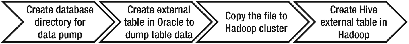
CopyToBDA utility workflow
- 1.
Copy to BDA utility works well for static tables whose data change rate is not frequent. Reason being it doesn’t allow the continuous refresh between source data and target.
- 2.
If the table size is large, data can be dumped in multiple .dmp files
- 3.For a Hive external table to access the dump files and prepare the result set, specify appropriate SerDe, InputFormat and OutputFormat
- a.
SERDE 'oracle.Hadoop.hive.datapump.DPSerDe'
- b.
INPUTFORMAT ‘oracle.Hadoop.hive.datapump.DPInputFormat’
- c.
OUTPUTFORMAT ‘org.apache.Hadoop.hive.ql.io.HiveIgnoreKeyTextOutputFormat’
- a.
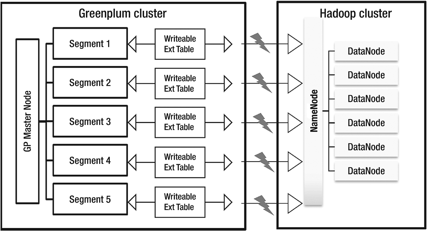
Greenplum gphdfs utility
Greenplum offers the gphdfs protocol to enable batched data transfer operations between the Greenplum and Hadoop clusters. For Greenplum as a source, the utility has been a de-facto mechanism for data movement as it fully exploits the MPP capability of the database. On the target side, it can work with various flavors of Hadoop like Cloudera, Hortonworks, MapR, Pivotal HD, and Greenplum HD.
The gphdfs utility must be setup on all segment nodes of a Greenplum cluster. During a data transfer operation, all segments concurrently push the local copies of data splits to the Hadoop cluster. The number of segment nodes in the Greenplum cluster measure the degree of parallelism of data transfer. Data distribution on segments plays a key role in determining the effort at a segment level process. If a table is unevenly distributed on the cluster, the gphdfs processes will have an irregular split size, which will impact the performance of the data ingestion process.
- 1.
Create repo file using
wget -nv http://public-repo-1.hortonworks.com/HDP/centos7/2.x/updates/2.6.1.0/hdp.repo - 2.
Install the libraries using YUM
yum install Hadoop Hadoop-hdfs Hadoop-libhdfs Hadoop-yarn Hadoop-mapreduce Hadoop-client openssl -y - 3.Set the Hadoop configuration parameters
- a.
gpconfig -c gp_Hadoop_home -v " '/usr/hdp/2.6.1.0-129'”
- b.
gpconfig -c gp_Hadoop_target_version -v "'hdp2'"
- c.
Set java home and Hadoop home
- a.
How GPHDFS utility works
- 1.
JVM and gphdfs – The gphdfs protocol uses JVM on each segment host to access and write data into HDFS. While the writable external table is created on segment host and accessed via gphdfs, each segment instance initializes the JVM process with 1GB of memory .
In case of high workloads during reading and writing multiple tables at the same time, JVM Heap memory issue might occur. You can decrease the value of the parameter GP_JAVA_OPT in $GPHOME/lib/Hadoop/Hadoop_env.sh from 1GB to 500MB.
- 2.Kerberos and gphdfs – The gphdfs protocol supports Kerberos authentication for Hadoop cluster. Kerberos authentication details are required to be updated in below files –
Yarn-site.xml
Core-site.xml
Hdfs-site.xml
In addition, the /etc/krb5.conf must be present in the Greenplum cluster. In case you are facing GSSAPI errors while accessing HDFS, install the Java Cryptography extension (JCE) on Greenplum nodes ($JAVA_HOME/jre/lib/security).
- 3.
Trigger gphdfs via ETL – The gphdfs utility can be embedded in Python script and fired through a standard ingestion tool like Informatica, Talend, Appworx, etc.
- 4.
The LOCATION parameter of the writable external table must have either the Hadoop cluster name or HDFS namenode’s hostname and port details.
- 5.
Compression support – Use compress and compression_type arguments in writable external table to load data in compressed format into HDFS.
- 6.
Custom loading framework is possible that loads group of tables (batch tables by schema or category) using python or any other scripting language
Data transfer from Greenplum to using gpfdist
In addition to gphdfs, the Greenplum utility gpfdist can be used to transfer the data from the Greenplum to HDFS.
The gpfdist utility offers parallel file operations in the Greenplum database. It can be used to move data from Greenplum segments to Hadoop clusters via edge node. You can create a writable external table in Greenplum using the below script.
- 1.
Use Hadoop put command to copy file in HDFS
- 2.
Secure copy (scp) the file to Hadoop name node
Ingest unstructured data into Hadoop
The technological and analytical advances sparked by machine textual analysis prompted many businesses to research applications, leading to the development of areas like sentiment analysis, speech mining, and predictive analytics. The emergence of Big Data in the late 2000s led to a heightened interest in the applications of unstructured data analytics in contemporary fields like natural language processing, and image or video analytics.
Unstructured data is information that either does not have a pre-defined data model or is not organized in a pre-defined manner. Unstructured information is typically text-heavy, but may contain data such as dates, numbers, and facts as well. This results in irregularities and ambiguities that make it difficult to understand using traditional programs as compared to data stored in fielded form in databases or annotated in documents.
Apache Flume
Apache Flume is a distributed system to capture and load large volumes of log data from different source systems to the data lake. Traditional solutions to copy a data set securely over network from one system to other, work only when data set is relatively small, easy and readily available. Given the challenges of a near real-time replication, batched loads, and volume, the urge to have a robust, flexible, and extensible tool cannot be ignored. Flume fits the bill appropriately as a reliable system that can transfer streaming events from different sources to HDFS.
Flume had its roots at Cloudera since 2011 and is packaged as a native component of Hadoop stack. It is used to collect and aggregate streaming data as events. Built upon a distributed pipeline architecture, the framework consists a Flume agent (or multiple independent federated agents) consisting of a channel that connects sources to sink. What flume guarantees is end-to-end reliability by enabling transactional exchange between agents and configurable data persistency characteristics of channels. The flume topology can be flexibly tweaked to optimize event volume and load balancing.
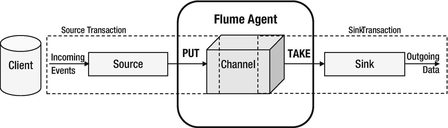
Apache Flume architecture
A flume event is a byte size data object, along with optional headers as key-value pair of distinctive information, transporting through the agent.
Source is a scalable component that accepts data from the data source and writes to the channel. It may, optionally, have an interceptor to modify events through tagging, filtering, or altering. Events pushed to the channel are PUT transactions.
The channel, depending on its configuration, queues the flume events persistently as received. It helps in persisting the events and controls fluctuations in data loads.
The sink pulls the data from channel and pushes to the target data store (could be HDFS or another flume agent). Events pulled by sink from the channel are TAKE transactions.
Data flow from source to sink is carried out using transactions which eliminates the risk of data loss in the pipeline. Flume works best for sources that generate streams of data at a steady rate. Source data can be synchronous like Avro, Thrift, spool directory, HTTP, Java message service, or asynchronous like SYSLOGTCP, SYSLOGUDP, NETCAT, or EXEC. For synchronous sources, client can handle failures, while for asynchronous, it cannot. Similarly, sinks can be HDFS, HBase (sync and async), Hive, logger, Avro, Thrift, File roll, morphlineSolr, ElasticSearch, Kafka, Kite, and more flume agents.
Tiered architecture for convergent flow of events
A tiered framework of multiple agents can be setup to enable convergent flow of events to multiple sinks. There can be multiple motivations behind the tiered approach. The primary motivation is to optimize the data volume distribution and insulate sinks from uneven data loads. Other reasons could be to relieve sources from holding large volumes of events for long time.
Loosely connected independent flume agents in the outermost tier (Tier-1) hold event streams from the sources. In the subsequent tier, sources consolidate the event streams received from preceding tier’s sinks. The process of consolidation and aggregation continues until the last tier, before the sinks in the innermost tier route the events to HDFS. Agent count is maximum in the outermost tier while event volume is highest in the innermost tier.

Apace Flume tiered model
A tiered architecture achieves load balancing and enables a distinguished layer between collector, storage, and aggregator agents.
Features and design considerations
- 1.Channel type – Flume has three built-in channels, namely, MEMORY, JDBC, and FILE.
- a.MEMORY – events are read from source to memory. Being a memory based operation, event ingestion is very fast. On contrary, since the changes captured are volatile in nature, incidents like agents crash or hardware issue can result into data loss. Business critical events are not a good choice but low category logs can be set of memory channel.
- i.
You can set the event capacity using agent.channels.c1.capacity. Java heap space should also be increased in accordance with the capacity.
- ii.
Use keep-alive to determine wait time for the process that writes event into the channel.
- iii.
Low put and take transaction latencies but not a cost-effective solution for a large event
- i.
- b.
FILE – events are read from source and written to files on a filesystem. Though slow, it is considered as durable and reliable option amongst the three channels as it uses Write Ahead Log mechanism along with storage directory to track events in the channel. Set the checkpointDir and dataDirs attributes of the channel to set directories where events are to be held.
- c.
JDBC – events are read and stored in Derby database. Enables ACID support as well but acute adoption trends due to performance issues.
- d.Kafka channel – events get stored in a Kafka topic in a cluster. This is one of the recent integrations that can be retrofitted into multiple scenarios:
- i.
Flume source and sink available – event written to Kafka topic
- ii.
Flume source – event captured in a Kafka topic. Integration with other applications is use-case driven.
- iii.
Flume sink – While Kafka captures the events from source systems, the sink helps in transporting events to HDFS, HBase, or Solr.
- i.
- a.
- 2.Channel capacity and transaction capacity – Channel capacity is the maximum number of events in a channel. Transaction capacity is the maximum number of events passed to a sink in single transaction. Attributes capacity and transactionCapacity are set for a channel.
- a.
Channel capacity must be large enough to queue many events. It depends on the size of an event, memory or disk size.
- b.
For MEMORY channel, channel capacity is limited by RAM size.
- c.
For FILE, channel capacity is limited by disk size.
- d.
Transaction capacity depends on batch size configured for the sinks
- a.
- 3.Event batch size – The transaction capacity or batch size is the maximum number of events that can be batched in a single transaction. It is set at the source and sink level.
- a.
Set at source – number of events in a batch written to channel
- b.
Set at sink – number of events captured by sink in single transaction before flush
- c.
Batch size <<channel>>.batchSize must be less than or equal to channel transaction capacity for proper resource management.
- d.
Larger the batch size at sink, faster the channels function to free up space for more events. For a file channel, post flush operation may be time consuming for fat batches.
- e.
Best practice to have transaction capacity that yields optimum performance. Not fixed formula but a gradual exercise.
- f.
If a batch fails in between, entire batch is replayed; which may cause duplicates at destination
- a.
- 4.
Channel selector ( Replicator/Multiplexer ) – An event in flume, can either be replicated to all channels or conditional-copied to selected channels. For instance, if an event to be consumed by HDFS, Kafka, HBase, and Spark, channels can be marked as replicator. Replication is the default channel selector type. If an event needs to be routed to different channels based on a rule or context, selected channels can be marked as multiplexer. Selector applies before event stream reaches the channel.
agent.sources.example.selector.type = multiplexingagent.sources.example.selector.mapping.healthy = mychannelagent.sources.example.selector.mapping.sick = yourchannelagent.sources.example.selector.default = mychannelagent.sources.example.selector.header = someHeaderIn case replicator and multiplexer do not suffice the requirements, custom replication strategy can also be developed.
- 5.
Channel provisioning – if the channels are insufficiently provisioned in the topology, it will create a bottleneck in the event flow, in terms of event load per agent and resource utilization.
- 6.
In a multi-hop flow or a tiered farm, keep note of the hops that an event makes before landing to destination. Note that the channels within the agents, at a given time, act as event buffers. In case of many hops, if any one agent goes faulty, the impact can get cascaded until source.
- 7.
Flume follows extensible framework. Custom flume components are required to add their jars to FLUME_CLASSPATH in flume-env.sh file. Other way is the plugins.d directory under $FLUME_HOME path. If plugins follow the defined format, flume-ng process will read the compatible plugins from plugins.d directory.
- 8.
Flume topology is highly dependent on use case. For a time-series evenly generating data, flume can work wonders. If source data pipeline is wrecked, flume is not a good choice as it might potentially break flume topology and cause prolonged outages. Frequent configuration changes to flume topology are not recommended.
- 9.
Due to global spread out, time zones have become indispensable piece of data ingestion strategy. All timings and schedules must be normalized a single time zone UTC in its standard format.
Conclusion
In this chapter, we discussed different approaches to bring data into a the Hadoop data lake. The chapter kicks off with the principles of ingestion framework and a quick brush up on basic ETL and ELT concepts. We discussed batched ingestion concepts and its design considerations. Under real-time processing, we explored how change data capture works and what its key drivers are in real-world scenarios. Key takeaways from this chapter would be two apache foundation products: sqoop and flume. Both have proved useful in integrating structured and unstructured data in data lake ecosystems.
In the next chapter, we’ll cover data streaming strategies, focusing majorly on Kafka.