© Banu Parasuraman 2023
B. ParasuramanPractical Spring Cloud Functionhttps://doi.org/10.1007/978-1-4842-8913-6_5

5. AI/ML Trained Serverless Endpoints with Spring Cloud Function

Banu Parasuraman1  
(1)
Frisco, TX, USA
 

This chapter looks at how Spring Cloud Function can be leveraged in AI/ML. You learn about the AI/ML process and learn where Spring Cloud Function fits in the process. You also learn about some of the offerings from the cloud providers, such as AWS, Google, and Azure.

Before delving into the details of Spring Cloud Function implementation, you need to understand the AI/ML process. This will set the stage for implementing Spring Cloud Function.

5.1 AI/ML in a Nutshell

AI/ML is gaining popularity, as it is being offered by almost all cloud providers. For AI/ML to work properly, it is important to understand the process behind it. See Figure 5-1.

A process of the M L lifecycle. The 4 processing steps are, gathering requirements, setting A I slash M L pipeline, performing A I slash M L, and monitoring.

Figure 5-1

ML lifecycle

Let’s dig deeper into the process depicted in Figure 5-1 and see what is accomplished.
  1. 1)
    Gathering requirements
    • Model requirements

      This is an important step in the AI/ML process. This determines the ultimate success or failure of the AI/ML model activity. The requirements for models must match the business objectives.

    • What is the return on investment (ROI) expected from this activity?

    • What are the objectives? Examples may include reduce manufacturing costs, reduce equipment failures, or improve operator productivity.

    • What are the features that need to be included in the model?

    • In character recognition, it can be histograms counting the number of black pixels along horizontal and vertical directions, the number of internal holes, and so on.

    • In speech recognition, it can be recognizing phonemes.

    • In computer vision, it can be a lot of features such as objects, edges, shape size, depth, and so on.

     
  1. 2)
    Setting up the data pipeline
    • Data collection
      1. i.

        What datasets to integrate

         
      2. ii.

        What are the sources

         
      3. iii.

        Are the datasets available

         
    • Data cleaning: This activity involves removing inaccurate or noisy records from the dataset. This may include fixing spelling and syntax errors, standardizing datasets, removing empty fields, and removing duplicate data. 45 percent of a data scientist’s time is spent on cleaning data (https://analyticsindiamag.com/data-scientists-spend-45-of-their-time-in-data-wrangling/).

    • Data labeling: Tagging or labeling raw data such as images, videos, text, audio, and so on, is an important part of the AI/ML activity. This makes the data meaningful and allows the machine learning model to identify a particular class of objects. This helps a lot in the supervised learning activities such as image classification, image segmentation, and so on.

     
  2. 3)
    Performing the AI/ML tasks
    • Feature engineering: This refers to all activities that are performed to extract and select features for machine learning models. This includes the use of domain knowledge to select and transform the most relevant variables from raw data to create predictive models. The goal of feature engineering is to improve the performance of machine learning algorithms. The success or failure of the predictive model is determined by feature engineering and ensure that the model will be comprehensible to humans.

    • Train model: In this step the machine learning algorithm is fed with sufficient training data to learn from. The training model dataset consists of sample output data and the corresponding sets of input data that influence the output. This is a iterative process that takes the input data through the algorithm and correlates it against the sample output. The result is then used to modify the model. This iterative process is called “model fitting” until the model precision meets the goals.

    • Model evaluation: This process involves using metrics to understand the model’s performance, including its strengths and weaknesses. For example, doing a classification prediction, the metrics can include true positives, true negatives, false positives, and false negatives. Other derived metrics can be accuracy, precision, and recall. Model evaluation allows you to determine how well the model is doing, the usefulness of the model, how additional model training will improve performance, and whether you should include more features.

    • Deploy model: This process involves deploying a model to a live environment. These models can then be exposed to other processes through the method of model serving. The deployment of models can involve a process of storing the models in a store such as Google Cloud Storage.

     
  3. 4)

    Monitoring the AI/ML models

    In this process, you want to make sure that the model is working properly and that the model predictions are effective. The reason you need to monitor model is that models may degrade over time due to these factors:

     
  • Variance in deployed data

  • Variance refers to the sensitivity of the learning algorithms to the training dataset. Every time you try to fit a model, the output parameters may vary ever so slightly, which will alter the predictions. In a production environment where the model has been deployed, these variances may have a significant impact if they’re not corrected in time.

  • Changes in data integrity

  • Machine learning data is dynamic and requires tweaking to ensure the right data is supplied to the model. There are three types of data integrity problems—missing values, range violations, and type mismatches. Constant monitoring and management of these types of issues is important for a good operational ML.

  • Data drift

  • Data drift occurs when the training dataset does not match the data output in production.

  • Concept drift

  • Concept drift is the change in relationships between input and output data over time. For example, when you are trying to predict consumer purchasing behavior, the behavior may be influenced by factors other than what you specified in the model. factors that are not explicitly used in the model prediction are called hidden contexts.

Let’s evaluate these activities from a compute perspective. This will allow us to determine what kind of compute elements we can assign to these process

Some of the activities in this process are short lived and some are long running process. For example, deploying models and accessing the deployed models is a short lived process. While Training models and model evaluation require both a manual and programmatic intervention and will take a lot of processing time.

Table 5-1 shows the type of compute that can be applied to the processes. Some of the processes are manual.
Table 5-1

Where to Use Spring Cloud Function in the AI/ML Process

AI/ML Process

Human

Compute


Spring Cloud Function (Short Run)

Batch (Long Run)

Model requirements

Human/manual process


Collect data


Integration triggers, data pipeline sources or sinks

Data pipeline process-Transformation

Data cleaning


Integration triggers

Transformation process

Data labeling


Tagging discrete elements-updates, deletes

Bulk tagging

Feature engineering

Manual


Train model


Trigger for training

Training process

Model evaluation

Manual

Triggers for evaluation

Bulk evaluation

Deploy models


Model serving, model

Bulk storage

Monitoring models


alerts


AI/ML processes require varying compute and storage requirements. Depending on the model size, the time taken to train, the complexity of the model, and so on, the process may require different compute and storage at different times. So, the environment should be scalable. In earlier days, AI/ML activities were conducted with a fixed infrastructure, through over-allocated VMs, dedicated bare metal servers, or parallel or concurrent processing units. This made the whole process costly and it was left to companies with deep pockets to be able to conduct proper AI/ML activities.

Today, with all the cloud providers providing some level of AI/ML activities through an API or SaaS approach, and with the ability to pay per use or pay as you go, companies small and big have begun to utilize AI/ML in their compute activities.

Paradigms such as cloud functions make it even easier to take advantage of a scalable platform offered by the cloud. Activities such as model storage and retrieval can be done on demand with cloud functions. Serving pre-trained models is easy through cloud functions and these models can be made available to any client without the need to install client libraries. Here are some of the advantages of cloud functions in AI/ML:
  • Codeless inference makes getting started easy

  • Scalable infrastructure

  • No management of infrastructure required

  • Separate storage for the model, which is very convenient for tracking versions of the model and for comparing their performance

  • Cost structure allows you to pay per use

  • Ability to use different frameworks

5.1.1 Deciding Between Java and Python or Other Languages for AI/ML

Most of the popular frameworks such as TensorFlow are written in Python, so the models’ outputs are also Python based. Therefore, it’s easy for anyone working on AI/ML to code in Python. See Figure 5-2.

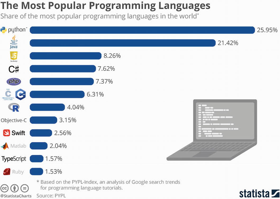
A pictorial horizontal bar graph of the most popular programming languages. It mentions the logo of worldwide languages with percentages and a laptop image. Python has the highest at 25.95 and Ruby, has the lowest at 1.53.

Figure 5-2

AI/ML language popularity

It is very important to understand that the popularity of a language does not equate to it being a good, robust, secure language for use in AI/ML.

There are several reasons to choose Java over Python or R:
  • Enterprises have standardized on Java, so they prefer to have their AI/ML platform written in Java to ease the integration into existing systems.

  • Apache.org , the open source community for Java, is very robust and has many libraries and tools that have been tuned toward speed of compute, data processing, and so on. Tools such as Hadoop, Hive, and Spark are integral to the AI/ML process. Developers can easily use these tools and libraries in their java code.

  • Java can be used at all touchpoints in the AI/ML process, including data collection, cleansing, labeling, model training, and so on. This way you can standardize on one language for AI/ML needs.

  • JVMs allow for applications to be portable across different machine types.

  • Due to Java’s object-oriented mechanisms and JVMs, it is easier to scale.

  • Java-based computation for AI/ML can be made to perform faster with some tuning at the algorithm and JVM level. Therefore, it is a preferred language for sites like Twitter, Facebook, and so on.

  • Java is a strong typing programming language, meaning developers must be explicit and specific about variables and types of data.

  • Finally, production codebases are often written in Java. If you want to build an enterprise-grade application, Java is the preferred language.

Since Java is a preferred enterprise language for AI/ML, we can safely say that Spring Cloud Function is a better framework to use when developing enterprise-grade functions for AI/ML.

This chapter explores the different offerings from the different cloud providers and explains how you can use Spring Cloud Function with these offerings.

5.2 Spring Framework and AI/ML

A lot of frameworks have been developed in Java that can be leveraged using the Spring Framework. The latest of these frameworks was developed by AWS and is called DJL (Deep Java Library). This library can integrate with PyTorch, TensorFlow, Apache MXNet, ONNX, Python, and TFLite based models.

One of the important capabilities that you need is model serving, where you can leverage Spring Cloud Function to serve trained models, and DJL provides this capability out of the box. It’s called djl-serving.

Spring Cloud Function is unique in its ability to transcend the on-premises and cloud, especially in the realm of AI/ML. Even though cloud has become popular, not all companies have fully transitioned to the cloud. Most of them in fact have adopted a hybrid approach. Some of the applications and data still reside in the company-owned datacenters or are co-hosted in datacenters operated by third-party service providers. AI/ML activities revolving the data that is residing in the datacenters will need to have models that are trained and stored and be served using cloud functions that can be hosted in the datacenter. Cloud functions hosted in the datacenter are nearer to their data and therefore have better performance than cloud functions that are hosted in the cloud and access models that are trained and stored in the on-premises datacenters. This is where Spring Cloud Function can help serve models on-premises. See Figure 5-3.

An illustrated model of the on-prem data center. The flow of data includes trained model data, the model serving, an enterprise application, a firewall, and an external application.

Figure 5-3

On-premises and Spring Cloud Function deployment for model serving

5.3 Model Serving with Spring Cloud Function with DJL

Before you explore the cloud provider’s option, it’s a good idea try this out locally. To do that, you need a framework installed and access to a good tensor model and an image. The framework that you use in this example is called djl-serving.

5.3.1 What Is DJL?

Deep Java Library (DJL) https://docs.djl.ai/ is a high-level, engine-agnostic Java framework for deep learning. It allows you to connect to any framework like TensorFlow or PyTorch and conduct AI/ML activities from Java.

DJL has also great hooks to Spring Boot and can easily be invoked through the Spring Framework. DJL acts as an abstraction layer across frameworks and makes it easy to interact with those frameworks, as shown in Figure 5-4.

A model of layers of the deep java library. It includes a java framework with a logo of spring boot, and spring cloud function. An M L framework of m x net, Tensor flow, PyTorch. Deep Lava Library is mentioned between the frameworks.

Figure 5-4

Deep Java Library (DJL) layers

There are many components in DJL that are useful to look at, but the DJL serving is interesting.

Run the following commands to get the djl-serving bits. Then unzip the file into your directory of choice and set the path to the serving.bat located at ~serving-0.19.0inserving.bat. This will allow you to execute serving from anywhere on your machine.
curl -O https://publish.djl.ai/djl-serving/serving-0.19.0.zip
unzip serving-0.19.0.zip
Listing 5-1 shows a sample run of djl-serving with a TensorFlow model.
# Load a TensorFlow model from TFHub
C:Usersanua>serving -m "resnet=https://tfhub.dev/tensorflow/resnet_50/classification/1"
[INFO ] - Starting djl-serving: 0.19.0 ...
[INFO ] -
Model server home: C:Usersanua
Current directory: C:Usersanua
Temp directory: C:UsersanuaAppDataLocalTemp
Command line:
Number of CPUs: 16
Max heap size: 8114
Config file: N/A
Inference address: http://127.0.0.1:8080
Management address: http://127.0.0.1:8080
Default job_queue_size: 1000
Default batch_size: 1
Default max_batch_delay: 300
Default max_idle_time: 60
Model Store: N/A
Initial Models: resnet=https://tfhub.dev/tensorflow/resnet_50/classification/1
Initial Workflows: N/A
Netty threads: 0
Maximum Request Size: 67108864
[INFO ] - Initializing model: resnet=https://tfhub.dev/tensorflow/resnet_50/classification/1
[INFO ] - Downloading https://publish.djl.ai/tensorflow-2.7.0/win/cpu/api-ms-win-core-synch-l1-2-0.dll.gz ...
[INFO ] - Downloading https://publish.djl.ai/tensorflow-2.7.0/win/cpu/api-ms-win-core-file-l1-2-0.dll.gz ...
[INFO ] - Downloading https://publish.djl.ai/tensorflow-2.7.0/win/cpu/THIRD_PARTY_TF_JNI_LICENSES.gz ...
[INFO ] - Downloading https://publish.djl.ai/tensorflow-2.7.0/win/cpu/api-ms-win-core-file-l1-1-0.dll.gz ...
[INFO ] - Downloading https://publish.djl.ai/tensorflow-2.7.0/win/cpu/api-ms-win-crt-environment-l1-1-0.dll.gz ...
[INFO ] - Downloading https://publish.djl.ai/tensorflow-2.7.0/win/cpu/api-ms-win-core-synch-l1-1-0.dll.gz ...
[INFO ] - Downloading https://publish.djl.ai/tensorflow-2.7.0/win/cpu/api-ms-win-core-string-l1-1-0.dll.gz ...
[INFO ] - Downloading https://publish.djl.ai/tensorflow-2.7.0/win/cpu/api-ms-win-core-memory-l1-1-0.dll.gz ...
[INFO ] - Downloading https://publish.djl.ai/tensorflow-2.7.0/win/cpu/msvcp140.dll.gz ...
[INFO ] - Downloading https://publish.djl.ai/tensorflow-2.7.0/win/cpu/api-ms-win-core-util-l1-1-0.dll.gz ...
[INFO ] - Downloading https://publish.djl.ai/tensorflow-2.7.0/win/cpu/api-ms-win-core-datetime-l1-1-0.dll.gz ...
[INFO ] - Downloading https://publish.djl.ai/tensorflow-2.7.0/win/cpu/vcruntime140.dll.gz ...
[INFO ] - Downloading https://publish.djl.ai/tensorflow-2.7.0/win/cpu/concrt140.dll.gz ...
[INFO ] - Downloading https://publish.djl.ai/tensorflow-2.7.0/win/cpu/api-ms-win-core-sysinfo-l1-1-0.dll.gz ...
[INFO ] - Downloading https://publish.djl.ai/tensorflow-2.7.0/win/cpu/ucrtbase.dll.gz ...
[INFO ] - Downloading https://publish.djl.ai/tensorflow-2.7.0/win/cpu/api-ms-win-core-interlocked-l1-1-0.dll.gz ...
[INFO ] - Downloading https://publish.djl.ai/tensorflow-2.7.0/win/cpu/api-ms-win-core-processenvironment-l1-1-0.dll.gz ...
[INFO ] - Downloading https://publish.djl.ai/tensorflow-2.7.0/win/cpu/api-ms-win-core-file-l2-1-0.dll.gz ...
[INFO ] - Downloading https://publish.djl.ai/tensorflow-2.7.0/win/cpu/tensorflow_cc.dll.gz ...
[INFO ] - Downloading https://publish.djl.ai/tensorflow-2.7.0/win/cpu/libiomp5md.dll.gz ...
[INFO ] - Downloading https://publish.djl.ai/tensorflow-2.7.0/win/cpu/vcomp140.dll.gz ...
[INFO ] - Downloading https://publish.djl.ai/tensorflow-2.7.0/win/cpu/api-ms-win-core-timezone-l1-1-0.dll.gz ...
[INFO ] - Downloading https://publish.djl.ai/tensorflow-2.7.0/win/cpu/jnitensorflow.dll.gz ...
[INFO ] - Downloading https://publish.djl.ai/tensorflow-2.7.0/win/cpu/api-ms-win-crt-convert-l1-1-0.dll.gz ...
[INFO ] - Downloading https://publish.djl.ai/tensorflow-2.7.0/win/cpu/api-ms-win-core-errorhandling-l1-1-0.dll.gz ...
[INFO ] - Downloading https://publish.djl.ai/tensorflow-2.7.0/win/cpu/api-ms-win-core-namedpipe-l1-1-0.dll.gz ...
[INFO ] - Downloading https://publish.djl.ai/tensorflow-2.7.0/win/cpu/api-ms-win-crt-math-l1-1-0.dll.gz ...
[INFO ] - Downloading https://publish.djl.ai/tensorflow-2.7.0/win/cpu/api-ms-win-crt-locale-l1-1-0.dll.gz ...
[INFO ] - Downloading https://publish.djl.ai/tensorflow-2.7.0/win/cpu/api-ms-win-crt-heap-l1-1-0.dll.gz ...
[INFO ] - Downloading https://publish.djl.ai/tensorflow-2.7.0/win/cpu/api-ms-win-core-profile-l1-1-0.dll.gz ...
[INFO ] - Downloading https://publish.djl.ai/tensorflow-2.7.0/win/cpu/LICENSE.gz ...
[INFO ] - Downloading https://publish.djl.ai/tensorflow-2.7.0/win/cpu/api-ms-win-crt-utility-l1-1-0.dll.gz ...
[INFO ] - Downloading https://publish.djl.ai/tensorflow-2.7.0/win/cpu/api-ms-win-core-heap-l1-1-0.dll.gz ...
[INFO ] - Downloading https://publish.djl.ai/tensorflow-2.7.0/win/cpu/api-ms-win-core-localization-l1-2-0.dll.gz ...
[INFO ] - Downloading https://publish.djl.ai/tensorflow-2.7.0/win/cpu/api-ms-win-core-debug-l1-1-0.dll.gz ...
[INFO ] - Downloading https://publish.djl.ai/tensorflow-2.7.0/win/cpu/api-ms-win-core-processthreads-l1-1-1.dll.gz ...
[INFO ] - Downloading https://publish.djl.ai/tensorflow-2.7.0/win/cpu/api-ms-win-core-libraryloader-l1-1-0.dll.gz ...
[INFO ] - Downloading https://publish.djl.ai/tensorflow-2.7.0/win/cpu/api-ms-win-crt-time-l1-1-0.dll.gz ...
[INFO ] - Downloading https://publish.djl.ai/tensorflow-2.7.0/win/cpu/api-ms-win-core-rtlsupport-l1-1-0.dll.gz ...
[INFO ] - Downloading https://publish.djl.ai/tensorflow-2.7.0/win/cpu/api-ms-win-crt-runtime-l1-1-0.dll.gz ...
[INFO ] - Downloading https://publish.djl.ai/tensorflow-2.7.0/win/cpu/api-ms-win-crt-stdio-l1-1-0.dll.gz ...
[INFO ] - Downloading https://publish.djl.ai/tensorflow-2.7.0/win/cpu/api-ms-win-core-console-l1-1-0.dll.gz ...
[INFO ] - Downloading https://publish.djl.ai/tensorflow-2.7.0/win/cpu/vcruntime140_1.dll.gz ...
[INFO ] - Downloading https://publish.djl.ai/tensorflow-2.7.0/win/cpu/api-ms-win-core-processthreads-l1-1-0.dll.gz ...
[INFO ] - Downloading https://publish.djl.ai/tensorflow-2.7.0/win/cpu/api-ms-win-core-handle-l1-1-0.dll.gz ...
[INFO ] - Downloading https://publish.djl.ai/tensorflow-2.7.0/win/cpu/api-ms-win-crt-filesystem-l1-1-0.dll.gz ...
[INFO ] - Downloading https://publish.djl.ai/tensorflow-2.7.0/win/cpu/api-ms-win-crt-multibyte-l1-1-0.dll.gz ...
[INFO ] - Downloading https://publish.djl.ai/tensorflow-2.7.0/win/cpu/api-ms-win-crt-string-l1-1-0.dll.gz ...
2022-09-21 12:09:38.465035: I external/org_tensorflow/tensorflow/core/platform/cpu_feature_guard.cc:151] This TensorFlow binary is optimized with oneAPI Deep Neural Network Library (oneDNN) to use the following CPU instructions in performance-critical operations:  AVX2
To enable them in other operations, rebuild TensorFlow with the appropriate compiler flags.
[INFO ] - initWorkers for resnet (cpu()): -1, -1
[INFO ] - Loading model resnet on cpu()
2022-09-21 12:09:38.595923: I external/org_tensorflow/tensorflow/cc/saved_model/reader.cc:43] Reading SavedModel from: C:Usersanua.djl.aicache epomodelundefinedaidjllocalmodelzooffdb59c80e9d66dc0ce00e409e06e710
2022-09-21 12:09:38.641647: I external/org_tensorflow/tensorflow/cc/saved_model/reader.cc:107] Reading meta graph with tags { serve }
2022-09-21 12:09:38.641933: I external/org_tensorflow/tensorflow/cc/saved_model/reader.cc:148] Reading SavedModel debug info (if present) from: C:Usersanua.djl.aicache epomodelundefinedaidjllocalmodelzooffdb59c80e9d66dc0ce00e409e06e710
2022-09-21 12:09:38.837590: I external/org_tensorflow/tensorflow/cc/saved_model/loader.cc:210] Restoring SavedModel bundle.
2022-09-21 12:09:39.330251: I external/org_tensorflow/tensorflow/cc/saved_model/loader.cc:194] Running initialization op on SavedModel bundle at path: C:Usersanua.djl.aicache epomodelundefinedaidjllocalmodelzooffdb59c80e9d66dc0ce00e409e06e710
2022-09-21 12:09:39.746608: I external/org_tensorflow/tensorflow/cc/saved_model/loader.cc:283] SavedModel load for tags { serve }; Status: success: OK. Took 1150043 microseconds.
[INFO ] - scanning for plugins...
[INFO ] - plug-in folder not exists:C:Usersanuaplugins
[INFO ] - 0 plug-ins found and loaded.
[INFO ] - Initialize BOTH server with: NioServerSocketChannel.
[INFO ] - BOTH API bind to: http://127.0.0.1:8080
[INFO ] - Model server started.
Listing 5-1

djl-serving Run with a Tensorflow Model

On the initial run, the model you specified will be loaded:
"resnet=https://tfhub.dev/tensorflow/resnet_50/classification/1"

On subsequent runs, the model server will be available at port 8080 at http://localhost:8080.

This example provides an image of kitten and it will try to recognize the kitten by providing output with probabilities:
$curl -O https://resources.djl.ai/images/kitten.jpg
This will show the image in Figure 5-5.

A photograph of a kitten with closed eyes and legs laid out.

Figure 5-5

Image of a kitten for the model to predict

Next, run the following and you will see the output with probabilities.

You provide the djl-serving instance that is running at http://localhost:8080/predictions with the kitten image that is located in the current directory, and you get a response shown in Figure 5-6, which shows that the image is probably a tabby cat. The probability is 0.4107377231121063. This is close.

A screenshot of the window. It has the class name and probability input and outputs. It represents the D J L results.

Figure 5-6

DJL results for the image

An X-ray image. It diagnosis the lungs using a saved model.

Figure 5-7

Xray image provided to the saved_model

Next, you see how you can use DJL to create a Spring Cloud Function to serve models.

5.3.2 Spring Cloud Function with DJL

For this example, we borrow an example from DJL called pneumonia detection. This sample is available at https://github.com/deepjavalibrary/djl-demo/tree/master/pneumonia-detection.

This example uses an Xray image from https://djlai.s3.amazonaws.com/resources/images/chest_xray.jpg.

It predicts using a model from https://djl-ai.s3.amazonaws.com/resources/demo/pneumonia-detection-model/saved_model.zip.

The Spring Cloud Function you create will take an image, load the model, and provide a prediction, as in the cat example.

Step 1: Create the Spring Cloud Function with DJL framework. Add dependencies to the Hadoop file.

Add the DJL highlighted dependencies along with spring-cloud-function-web and GCP dependencies, as shown in Listing 5-2.
       <dependencies>
        <dependency>
            <groupId>org.springframework.boot</groupId>
            <artifactId>spring-boot-starter-web</artifactId>
        </dependency>
        <dependency>
            <groupId>org.springframework.cloud</groupId>
            <artifactId>spring-cloud-function-web</artifactId>
        </dependency>
        <!-- https://mvnrepository.com/artifact/ai.djl/bom -->
        <dependency>
            <groupId>ai.djl</groupId>
            <artifactId>bom</artifactId>
            <version>0.12.0</version>
            <type>pom</type>
        </dependency>
        <dependency>
            <groupId>ai.djl</groupId>
            <artifactId>api</artifactId>
            <version>0.12.0</version>
        </dependency>
        <dependency>
            <groupId>ai.djl.tensorflow</groupId>
            <artifactId>tensorflow-api</artifactId>
            <version>0.12.0</version>
        </dependency>
        <dependency>
            <groupId>ai.djl.tensorflow</groupId>
            <artifactId>tensorflow-engine</artifactId>
            <version>0.12.0</version>
        </dependency>
        <dependency>
            <groupId>ai.djl.tensorflow</groupId>
            <artifactId>tensorflow-native-auto</artifactId>
            <version>2.4.1</version>
            <scope>runtime</scope>
        </dependency>
        <dependency>
            <groupId>org.projectlombok</groupId>
            <artifactId>lombok</artifactId>
            <optional>true</optional>
        </dependency>
Listing 5-2

Dependencies for DJL

Step 2: Create the Spring Cloud Function.

Now create an XRAYFunction that stores a model from the URL provided: https://djl-ai.s3.amazonaws.com/resources/demo/pneumonia-detection-model/saved_model.zip. See Listing 5-3.
package com.kubeforce.djlxray;
import ai.djl.inference.Predictor;
import ai.djl.modality.Classifications;
import ai.djl.modality.cv.Image;
import ai.djl.modality.cv.ImageFactory;
import ai.djl.modality.cv.translator.ImageClassificationTranslator;
import ai.djl.modality.cv.util.NDImageUtils;
import ai.djl.repository.zoo.Criteria;
import ai.djl.repository.zoo.ZooModel;
import ai.djl.translate.Translator;
import lombok.SneakyThrows;
import org.slf4j.Logger;
import org.slf4j.LoggerFactory;
import java.io.IOException;
import java.util.Arrays;
import java.util.List;
import java.util.Map;
import java.util.function.Function;
public class XRAYFunction implements Function<Map<String,String>, String> {
    private static final Logger logger = LoggerFactory.getLogger(XRAYFunction.class);
    private static final List<String> CLASSES = Arrays.asList("Normal", "Pneumonia");
    String imagePath;
    String savedModelPath;
    @SneakyThrows
    @Override
    public String apply(Map<String, String> imageinput) {
            imagePath= imageinput.get("url");
            savedModelPath = imageinput.get("savedmodelpath");
            Image image;
            try {
                image = ImageFactory.getInstance().fromUrl(imagePath);
            } catch (IOException e) {
                throw new RuntimeException(e);
            }
            Translator<Image, Classifications> translator =
                    ImageClassificationTranslator.builder()
                            .addTransform(a -> NDImageUtils.resize(a, 224).div(255.0f))
                            .optSynset(CLASSES)
                            .build();
            Criteria<Image, Classifications> criteria =
                    Criteria.builder()
                            .setTypes(Image.class, Classifications.class)
//                           .optModelUrls("https://djl-ai.s3.amazonaws.com/resources/demo/pneumonia-detection-model/saved_model.zip")
                            .optModelUrls(savedModelPath)
                            .optTranslator(translator)
                            .build();
            try (ZooModel<Image, Classifications> model = criteria.loadModel();
                 Predictor<Image, Classifications> predictor = model.newPredictor()) {
                Classifications result = predictor.predict(image);
                logger.info("Diagnose: {}", result);
                return result.toJson();
            }
        }
    }
Listing 5-3

XRAYFunction.java

Step 3: Test locally. Run the Spring Cloud Function and invoke the endpoint http://localhost:8080/xrayFunction

Provide input:
 {
"url":"https://djl-ai.s3.amazonaws.com/resources/images/chest_xray.jpg",
"savedmodelpath":https://djl-ai.s3.amazonaws.com/resources/demo/pneumonia-detection-model/saved_model.zip
}
This is executed in Postman, as shown in Figure 5-8.

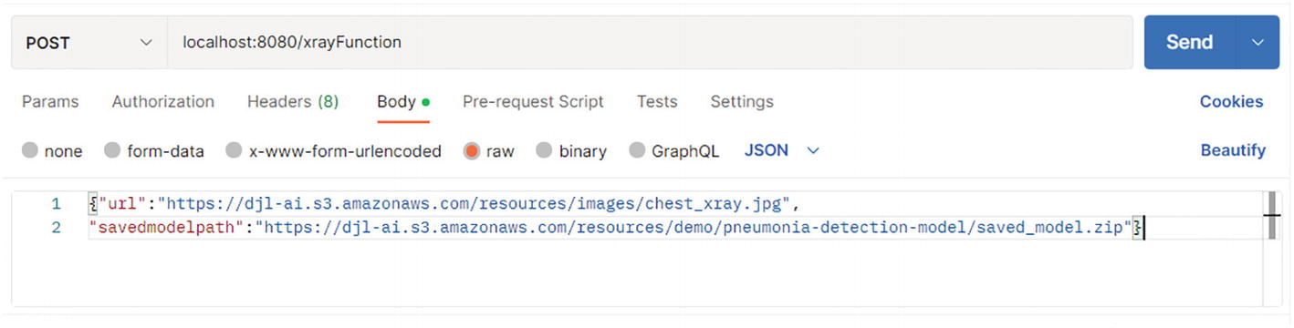
A screenshot of the postman testing. It highlights the local host, body, and row options with a testing program.

Figure 5-8

Testing with a POST in Postman

Upon invoking the function, the model is downloaded and then loaded into memory. This takes about a minute to load, after which it comes back with a successful message. The model took 802066 microseconds (80 seconds) to load, and this is critical for your function calls, as you will have to accommodate for this model-loading time. See Figure 5-9.

A screenshot of programming functions with number, date, and time. It represents the results from image evaluation.

Figure 5-9

Prediction results from the image evaluation

A flow diagram of the saved model. It classifies as training and deployment. It represents the tensor flow components. The output from the training is sent to the saved model and further to the deployment.

Figure 5-10

TensorFlow components1

This section successfully demonstrated that Spring Cloud Function can act as a model server in AI/ML. This is a critical function, as you can move the loading and serving of models from traditional servers to a function-based, “pay-per-use” model.

You also learned how to use deep learning Java libraries in your functions. You can deploy this Spring Cloud Function to any cloud, as shown in Chapter 2.

5.4 Model Serving with Spring Cloud Function with Google Cloud Functions and TensorFlow

This section explores the model serving on Google. It uses TensorFlow, which is a Google product from AI/ML and explains how to build and save an AI model with datasets such as MNIST (https://en.wikipedia.org/wiki/MNIST_database).

5.4.1 TensorFlow

TensorFlow was developed by Google and is an open source platform for machine learning. It is an interface for expressing and executing machine learning algorithms. The beauty of TensorFlow is that a model expressed in TensorFlow can be executed with minimal changes on mobile devices, laptops, or large-scale systems with multiple GPUs and CPUs. TensorFlow is flexible and can express a lot of algorithms, including training and inference algorithms for deep neural networks, speech recognition, robotics, drug discovery, and so on.

In Figure 5-9, you can see that TensorFlow can be deployed to multiple platforms and has many language interfaces. Unfortunately, TensorFlow is written in Python, so most of the models are written and deployed in Python. This poses a unique challenge for enterprises who have standardized on Java.

Even though TensorFlow is written in Python, there are lots of frameworks written in Java that work on a saved model.

Let’s look at how you can work with TensorFlow on the Google Cloud platform.

Google Cloud provides different approaches to working on models. You can use a container- or Kubernetes-based approach, an SaaS-based approach, or a Cloud Functions-based approach. Each has advantages and disadvantages. Google has published a good guide for you to pick the right platform for your needs, as shown in Table 5-2.
Table 5-2

Google and AI/ML Environment2

A table with 4 columns and 6 rows. The column headers are the features, compute engine, A L platform prediction, and cloud functions. It categorizes features and descriptions.

As you can see from Table 5-2, cloud functions are recommended for experimentation. Google recommends Compute Engine with TF Serving, or its SaaS platform (AI Platform) for predictions for production deployments.

The issue with this approach is that a function-based approach is more than just an experimentation environment. Functions are a way of saving on cost while exposing the serving capabilities for predictions through APIs. It is a serverless approach, so enterprises do not have to worry about scaling.

5.4.2 Example Model Training and Serving

In this section you see how to train an AI model locally and upload it to Google Cloud Storage. You will then download the model and test an image through a Cloud Function API. You will use a model that is based on MNIST. More about MNIST can be found at https://en.wikipedia.org/wiki/MNIST_database.

In this example, you develop the model in Python and then expose the model through Spring Cloud Function using DJL; see Figure 5-11.

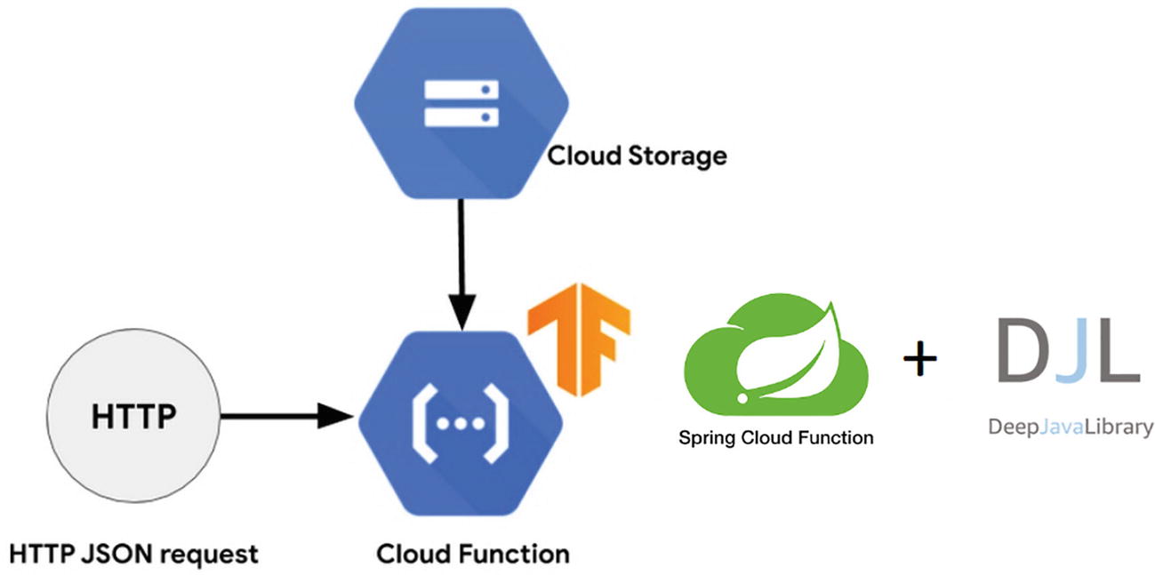
A model of spring cloud function. It indicates the tensor flow of H T T P J SON request, cloud storage, and cloud function with two logos of spring cloud function, and deep java library.

Figure 5-11

Spring Cloud Function with DJL and TensorFlow

You use the same example outlined at https://cloud.google.com/blog/products/ai-machine-learning/how-to-serve-deep-learning-models-using-tensorflow-2-0-with-cloud-functions. This will allow you to concentrate more on the Spring Cloud Function code that you will be creating rather than the actual implementation in Python.

You will then serve the model using Spring Cloud Function.

Step 1: Install TensorFlow.
python3 -m pip install tensorflow

Step 2: Create a project. Create a project called MNIST and then create a main.py file with the code in Listing 5-4. I used PyCharm to run this code.

On your Mac, make sure to run this command before running the code; otherwise you will get a certificate error. The code tries to download packages from googleapis:
open /Applications/Python 3.7/Install Certificates.command
I ran main.py and the whole process took me 13 minutes. At the end of it, I was able to get two model files as output.
from __future__ import absolute_import
from __future__ import division
from __future__ import print_function
from __future__ import unicode_literals
import tensorflow as tf
from tensorflow.keras.layers import Dense, Flatten, Conv2D
from tensorflow.keras import Model
EPOCHS = 10
mnist = tf.keras.datasets.mnist
fashion_mnist = tf.keras.datasets.fashion_mnist
(x_train, y_train), (x_test, y_test) = fashion_mnist.load_data()
x_train, x_test = x_train / 255.0, x_test / 255.0
# Add a channels dimension e.g. (60000, 28, 28) => (60000, 28, 28, 1)
x_train = x_train[..., tf.newaxis]
x_test = x_test[..., tf.newaxis]
train_ds = tf.data.Dataset.from_tensor_slices(
    (x_train, y_train)).shuffle(10000).batch(32)
test_ds = tf.data.Dataset.from_tensor_slices((x_test, y_test)).batch(32)
class CustomModel(Model):
    def __init__(self):
        super(CustomModel, self).__init__()
        self.conv1 = Conv2D(32, 3, activation='relu')
        self.flatten = Flatten()
        self.d1 = Dense(128, activation='relu')
        self.d2 = Dense(10, activation='softmax')
    def call(self, x):
        x = self.conv1(x)
        x = self.flatten(x)
        x = self.d1(x)
        return self.d2(x)
model = CustomModel()
loss_object = tf.keras.losses.SparseCategoricalCrossentropy()
optimizer = tf.keras.optimizers.Adam()
train_loss = tf.keras.metrics.Mean(name='train_loss')
train_accuracy = tf.keras.metrics.SparseCategoricalAccuracy(name='train_accuracy')
test_loss = tf.keras.metrics.Mean(name='test_loss')
test_accuracy = tf.keras.metrics.SparseCategoricalAccuracy(name='test_accuracy')
@tf.function
def train_step(images, labels):
    with tf.GradientTape() as tape:
        predictions = model(images)
        loss = loss_object(labels, predictions)
    gradients = tape.gradient(loss, model.trainable_variables)
    optimizer.apply_gradients(zip(gradients, model.trainable_variables))
    train_loss(loss)
    train_accuracy(labels, predictions)
@tf.function
def test_step(images, labels):
    predictions = model(images)
    t_loss = loss_object(labels, predictions)
    test_loss(t_loss)
    test_accuracy(labels, predictions)
for epoch in range(EPOCHS):
    for images, labels in train_ds:
        train_step(images, labels)
    for test_images, test_labels in test_ds:
        test_step(test_images, test_labels)
    template = 'Epoch {}, Loss: {}, Accuracy: {}, Test Loss: {}, Test Accuracy: {}'
    print(template.format(epoch + 1,
                          train_loss.result(),
                          train_accuracy.result() * 100,
                          test_loss.result(),
                          test_accuracy.result() * 100))
# Save the weights
model.save_weights('fashion_mnist_weights')
tf.saved_model.save(model, export_dir="c://Users//banua//Downloads/MNIST/models")
Listing 5-4

main.py

The key is tf.saved_model.save(model, export_dir="c://Users//banua//Downloads/MNIST/models").

This will save the model so that any model server can use it.

Step 3: Run the project.

Execute main.py from the IDE. See Figure 5-12.

A screenshot of the window. It represents the successful run of M N I S T. The pop-up text reads as generated model files located in the root of the project.

Figure 5-12

Successful run of MNIST and model building

Zip the assets, variables, and the saved_model.pb. file as Savedmodel3.zip and upload it to the Google Cloud Storage.

Step 4: Upload the models into Cloud Storage. Navigate to your Google Cloud Console and subscribe to Cloud Storage. It is available at cloud.google.com.

Create a storage bucket in Google Cloud Storage and upload the two files into the storage bucket. Use the defaults for this example. If you are using free credits from Google, this storage should be covered.

I created a bucket called mnist-soc. You will use the bucket name in the Cloud Functions call. See Figure 5-13.

A screenshot of the Google cloud storage bucket. It includes the name of the bucket, choosing store data, choosing default storage, choosing control access, and protecting access with highlighted lines.

Figure 5-13

Google Cloud Storage Bucket creation steps

Name your bucket mnist-soc and leave the others set to the defaults; then click Create.

Upload the savedmodel3.zip file to this folder by clicking Upload Files. See Figure 5-14.

A screenshot of a mnist soc application. It highlights the object option and mentions the model's name, size, and type. It represents the models located in cloud storage.

Figure 5-14

Models deployed into Cloud Storage

Click the file to get the details of the URL you need to connect to, as shown in Figure 5-15.

A screenshot represents the U R L for a model. It indicates a mnist soc application with a live object option. It highlights the public and authentication U R L with a link.

Figure 5-15

URL for the savedmodel3.zip

The URL you use for testing this example is https://storage.googleapis.com/mnist-soc/savedmodel3.zip.

The test image you use for this example is https://storage.googleapis.com/mnist-soc/test.png.

Note that the function that you created in Section 5.2 will be deployed in Step 5. If you use savedmodel3.zip and test.png, it will fail. But you will know that the function is working because you will get an error message that the model could not be loaded. This is an acceptable outcome for the model you created.

Step 5: Deploy the Spring Cloud Function to Google Functions. In this step, you take the function you created in Section 5.2 and deploy it into the Google Cloud Functions environment. The prerequisites and steps are the same as discussed in Chapter 2.

Prerequisites:
Modify the Spring Cloud Function to fit the Google Cloud Functions environment. See Listing 5-5.
<dependency>
    <groupId>org.springframework.cloud</groupId>
    <artifactId>spring-cloud-function-adapter-gcp</artifactId>
</dependency>
<dependencyManagement>
        <dependencies>
            <dependency>
                <groupId>org.springframework.cloud</groupId>
                <artifactId>spring-cloud-dependencies</artifactId>
                <version>${spring-cloud.version}</version>
                <type>pom</type>
                <scope>import</scope>
            </dependency>
            <dependency>
                <groupId>com.google.cloud</groupId>
                <artifactId>spring-cloud-gcp-dependencies</artifactId>
                <version>3.3.0</version>
                <type>pom</type>
                <scope>import</scope>
            </dependency>
        </dependencies>
    </dependencyManagement>
<build>
        <plugins>
            <plugin>
                <groupId>org.springframework.boot</groupId>
                <artifactId>spring-boot-maven-plugin</artifactId>
                <configuration>
                    <outputDirectory>target/deploy</outputDirectory>
                </configuration>
                <dependencies>
                    <dependency>
                        <groupId>org.springframework.cloud</groupId>
                        <artifactId>spring-cloud-function-adapter-gcp</artifactId>
                        <version>3.2.7</version>
                    </dependency>
                </dependencies>
            </plugin>
            <plugin>
                <groupId>com.google.cloud.functions</groupId>
                <artifactId>function-maven-plugin</artifactId>
                <version>0.9.1</version>
                <configuration>
                    <functionTarget>org.springframework.cloud.function.adapter.gcp.GcfJarLauncher</functionTarget>
                    <port>8080</port>
                </configuration>
            </plugin>
        </plugins>
    </build>
Listing 5-5

Dependencies for GCP Added

Deploy the Spring Cloud Function to Google Cloud Functions. Make sure that you build and package before you run the following command. A JAR file must be present in the target/deploy directory in the root of your project.

The saved model that you are going to test with is 400MB, so you have to accommodate this by increasing the memory to 4096 and setting the timeout to 540 seconds:
gcloud functions deploy DJLXRay-GCP --entry-point org.springframework.cloud.function.adapter.gcp.GcfJarLauncher --runtime java11 --trigger-http --source target/deploy --memory 4096MB --timeout 540
Once this runs successfully, you will get the output shown in Figure 5-16.

A screenshot of multiple programming functions. It denotes the deployed function, memory, and time.

Figure 5-16

Successfully deployed function with the specifed memory and timeout

Navigate to your Google Cloud Functions console to verify and to get the URL to test. See Figure 5-17.

A screenshot includes functions and cloud functions in the console. It highlights the create function and refresh. It indicates a filter option with details of the first gen.

Figure 5-17

Function shows up in the console

You now test in the Cloud Function console by providing input (see Figure 5-18). Note that you have to increase the memory to 4096MB with a timeout set to 540s just to be safe:
{"url":"https://djl-ai.s3.amazonaws.com/resources/images/chest_xray.jpg",
"savedmodelpath":"https://storage.googleapis.com/mnist-soc/saved_model.zip"}

A screenshot highlights the cloud function, D J L X ray -G C P. The testing option with Test the function is highlighted. The test was successfully executed.

Figure 5-18

Successful execution of the test

If you scroll down the test console, you get the execution times. This shows that the function execution took 16392ms, as shown in Figure 5-19. This is 16s for execution, which is phenomenal. This is faster because you stored the saved model in Google Cloud Storage, which is closer to the function.

A screenshot of the window denotes the multiple output logs. It highlights one log code no-16392, code- 200 with box .It displays the execution time.

Figure 5-19

Logs show the execution times

This section explored the capabilities of TensorFlow and explained how you can use DJL and Spring Cloud Function together to access a saved TensorFlow model. DJL makes it easy for Java programmers to access any of the saved models generated using Python frameworks, such as PyTorch (pytorch.org) and TensorFlow.

You also found that you have to set the memory and timeout based on the saved model size and store the model closer to the function, such as in Google’s storage offerings.

5.5 Model Serving with Spring Cloud Function with AWS Lambda and TensorFlow

This section emulates what you did in Chapter 2 for Lambda. It is best to finish that exercise before trying this one.

The prerequisites are the same as in Chapter 2. Here they are for your reference:

Step 1: Prep your Lambda environment. Ensure that you have access and a subscription to the AWS Lambda environment.

Step 2: Modify the Spring Cloud Function to fit the AWS Lambda environment. You need to add the DJL dependencies to the pom.xml file that you created in Chapter 2; see Listing 5-6.
<dependency>
            <groupId>ai.djl</groupId>
            <artifactId>api</artifactId>
            <version>0.12.0</version>
        </dependency>
        <dependency>
            <groupId>ai.djl.tensorflow</groupId>
            <artifactId>tensorflow-api</artifactId>
            <version>0.12.0</version>
        </dependency>
        <dependency>
            <groupId>ai.djl.tensorflow</groupId>
            <artifactId>tensorflow-engine</artifactId>
            <version>0.12.0</version>
        </dependency>
        <dependency>
            <groupId>ai.djl.tensorflow</groupId>
            <artifactId>tensorflow-native-auto</artifactId>
            <version>2.4.1</version>
            <scope>runtime</scope>
        </dependency>
        <dependency>
            <groupId>org.projectlombok</groupId>
            <artifactId>lombok</artifactId>
            <optional>true</optional>
        </dependency>
Listing 5-6

DJL Dependencies

Step 3: Deploy the Spring Cloud Function to Lambda. You should follow the process outlined in Chapter 2 to build and package the Spring Cloud Function and deploy it to Lambda.

Step 4: Test. Once you deploy the function to Lambda, test it with Postman. You should get the result shown in Figure 5-20.

A screenshot of the window of the successful execution. It highlights the body and pretty options and mentions the class name with probability.

Figure 5-20

Successful execution

5.6 Spring Cloud Function with AWS SageMaker or AI/ML

This section explores the offering from AWS called SageMaker and shows how you can use Spring Cloud Function with it.

AWS SageMaker (https://aws.amazon.com/sagemaker/) is a comprehensive platform for AI/ML activities. It is like a one-stop shop for creating and deploying ML models. Figure 5-21 shows AWS SageMaker’s flow.

A model of the A W S sage maker. The process includes labeling data, building, training, tuning, deploying, and discovering. Each step has a logo associated with it.

Figure 5-21

AWS SageMaker flow

SageMaker allows you to build and deploy models with Python as the language of choice, but when it comes to endpoints, there are Java SDKs much like AWS Glue that create prediction APIs or serve models for further processing. You can leverage Lambda functions for these APIs.

So, as you saw in TensorFlow, you have to work in Python and Java to model and expose models for general-purpose use.

Let’s run through a typical example and see if you can then switch to exposing APIs in Spring Cloud Function.

Note

This example uses the same sample to build, train, and deploy as in this hands-on tutorial in AWS.

https://aws.amazon.com/getting-started/hands-on/build-train-deploy-machine-learning-model-sagemaker/

Step 1: Create a notebook instance. Log on to SageMaker and create a notebook instance, as shown in Figure 5-22. Note: It is assumed that you have walked through the tutorial that Amazon provided.

A screenshot of the create notebook instance. It includes Notebook instance settings, Permissions, and encryption. It asks for the notebook instance name, type, elastic inference, platform identifier, and I A M role.

Figure 5-22

Notebook instance in SageMaker with properties set

Your notebook instance will be created, as shown in Figure 5-23.

A screenshot of the deployment of the notebook. It highlights the amazon sage maker and search notebook instance. It asks for name, instance, creation time, status, and actions.

Figure 5-23

Successful deployment of the notebook

Step 2: Prepare the data. Use Python to prepare the data. This example uses the XGBoost ML algorithm. See Figure 5-24.

A screenshot of the jupyter notebook. It highlights the option for new notebooks. It has the title files, running, cluster, sage maker example, and conda.

Figure 5-24

Pick a framework in the Jupyter notebook

As you can see from the list, most frameworks use Python. This example uses conda_python3, as suggested in the AWS tutorial.

Copy and paste the Python code into the Jupyter notebook cell and run it. You will get a “success” message, as shown in Figure 5-25.

A screenshot of the window of the Jupyter notebook code. It creates a sage maker for instance. In this program, the log mentions import libraries, defines I A M role, X G boost container.

Figure 5-25

Code to create a SageMaker instance

Copy and paste the code to create the s3 bucket to store your model, as shown in Figure 5-26.

A screenshot of the window for the creation of a bucket. This program includes the bucket name, steps, and process. The bucket was created successfully.

Figure 5-26

Create a bucket

Now copy and paste the code to download data into a dataframe, as shown in Figure 5-27.

A screenshot of the window for downloading the data to a data frame. The program includes the process of trying, except, and printing data.

Figure 5-27

Download the data into a dataframe

Scuffle and split the dataset, as shown in Figure 5-28.

A screenshot of the window for the work on the dataset. The program includes splitting the dataset to train data, test data, split data, and print.

Figure 5-28

Work on the dataset

Step 3: Train the model. See Figure 5-29.

A screenshot of the window for inputs and outputs. It indicates the training of the model with 3 steps.

Figure 5-29

Train the model

You have to wait for Step 3 to finish before deploying the model; see Figure 5-30.

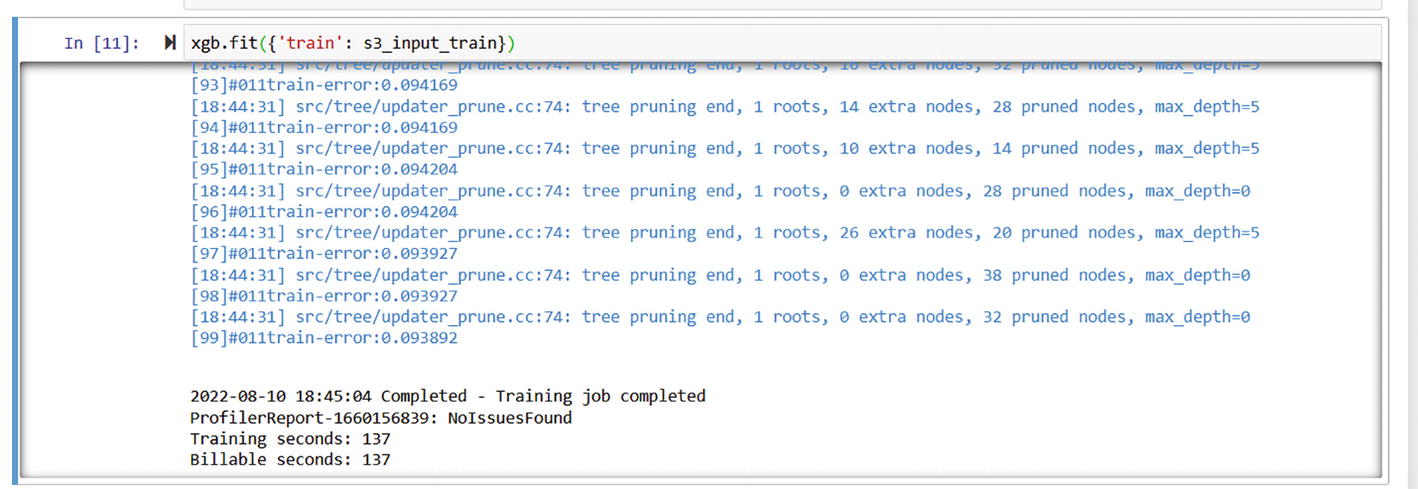
A screenshot of the window with the input and outputs. It indicates the S 3 training completion. It mentions that the training job was completed.

Figure 5-30

Training is complete

Step 4: Deploy the model. Make a note of the compute sizes used. This will impact your billing. See Figure 5-31.

A screenshot of the window for the deployment of the model. It indicates the programming function.

Figure 5-31

Deploy the model

Step 5: Make a note of the endpoints. See Figures 5-32 and 5-33.

A screenshot of the window of Amazon sage maker. It has endpoints that include the name, A R N, creation time, status, and last update.

Figure 5-32

Endpoint of the deployment

A screenshot of the window indicates the endpoint settings. It includes the name, type, A R N, creation time, status, last updated, U R L.

Figure 5-33

Details of the endpoint

Step 6: Create the Spring Cloud Function code to access the endpoint. Listing 5-7 shows the POM dependencies.
<dependency>
   <groupId>com.amazonaws</groupId>
   <artifactId>aws-java-sdk-sagemakerruntime</artifactId>
   <version>1.11.979</version>
   <exclusions>
      <exclusion>
         <groupId>com.amazonaws</groupId>
         <artifactId>aws-java-sdk-core</artifactId>
      </exclusion>
   </exclusions>
</dependency><dependency>
   <groupId>com.amazonaws</groupId>
   <artifactId>aws-java-sdk-core</artifactId>
   <version>1.11.979</version>
</dependency>
Listing 5-7

AWS SDK Dependencies

Create a Supplier class to call and get the result from the SageMaker endpoint. The SupplierFunction, unlike discussed in Section 5.3, will invoke an endpoint URL and provide the results. Here, you use SageMaker’s own model-serving capabilities. The Spring Cloud Function acts as a client for SageMaker. See Figure 5-34.

A screenshot of the window with the programming function input and output components. It represents the sage maker supplier in Java.

Figure 5-34

SageMakerSupplier.java

Deploy the function in Lambda, as shown in Chapter 2.

This section explained how to create and deploy a model in AWS SageMaker. You then called the SageMaker endpoint using the SageMaker JDK client in the Spring Cloud Function, which was deployed in AWS Lambda.

The Java-based Lambda function can be tuned to be more responsive and have a shorter cold startup time by using mechanisms such GraalVMs.

5.7 Summary

As you learned in this chapter, you can serve models using Spring Cloud Function. But you also learned that serving models using Spring Cloud Function and Java is a stretch because the AI/ML models are written in Python. While Python may be popular, it is also important to note that in an enterprise, Java is king. Finding ways to leverage Java in AI/ML is the key to having an integrated environment within your enterprise. Cold starts of Python-based functions take a long time. This is where using Java and frameworks such as GraalVM speeds up the startup times.

The next chapter explores some real-world use cases of IoT and Conversation AI and explains how Spring Cloud Function can be used.

..................Content has been hidden....................

You can't read the all page of ebook, please click here login for view all page.
Reset
13.58.82.79