OLAP

The term ‘online analytical processing’ (OLAP) has been applied to a range of techniques that can be used by senior managers and knowledge workers to query historical, summarised, multidimensional data. The term is used in contrast to ‘ online transactional processing’ (OLTP), where front-line staff are interacting with databases in the course of day-to-day operations. The data associated with OTLP is current, up to date and, probably, relational.

OLAP techniques provide the ability to answer more sophisticated questions than those provided by the standard reporting tools, such as ‘what if …?’ and ‘why …?’ A typical question would be ‘What will happen to our sales figures if we withdraw 200g tins of Brand X Baked Beans from our product range?’ The OLAP techniques are based around four basic operations that can be applied to a multidimensional cube of data: slice, dice, roll-up and drill-down.

The slice operation provides a sub-cube of data by selecting a subset of one of the dimensions. Slicing along the store dimension provides a sub-cube that contains data for a single store or a group of stores (for example, Store 315 or all the stores in the northern region, but showing the values for each product in the product range at each time period in the time range). Slicing along the product dimension provides a sub-cube that contains data for a single product or a category of products (for example, 200g tins of Brand X Baked Beans or all canned goods, but showing the values for each store at each time period in the time range). Slicing along the time dimension provides a sub-cube that contains data for a single time period (for example, 2–3pm on Friday 20 January 2007 or the whole of the first quarter 2007, but showing the values for each product in the product range sold at each store). Slicing purely selects a subset of the data that was available in the original cube without changing any of the values.

The dice operation provides a sub-cube of data by selecting a subset of two or more of the dimensions. The resultant sub-cube may, for example, contain data for a single store for a limited product range over a limited time period (for example, the value of sales of each product within the tinned goods category at Store 315 during January 2007). As with the slice operation, dicing purely selects a subset of the data that was available in the original cube without changing any of the values.

The roll-up (or aggregation) operation provides a new cube of data with the values along one or more dimensions aggregated; for example, rolling up along the product dimension gives a cube showing the total values for the sales for all products in each store in each time period. Unlike the slicing and dicing operations, the roll-up operation calculates new values.

The drill-down (or de-aggregation) operation provides a new cube of data with a more detailed view of the data along one or more dimensions. When drilling down the new cube is not formed from the existing cube of data (as it is for slice, dice and roll-up operations) but is formed from more detailed data; the assumption is that the original cube was showing aggregated data and more detailed data is held in the data warehouse. For example, if we have a cell showing, as a single value, the value of all the sales for tinned goods in all the stores in the northern region on Friday 20 January 2007, we can drill down to look at the sales by individual store, for each individual product or for each hour of the day, or for any combination of these three.

Data mining

Data mining is the application of advanced statistical and other techniques against the large volumes of data held in a data warehouse to discover previously unknown patterns in the data that may be of interest to the business. The patterns are discovered by identifying the underlying rules and features in the data. Data mining is sometimes known as knowledge discovery in databases (KDD). The techniques used in data mining include, amongst others, statistical techniques, cluster analysis and neural networks.

Statistical techniques can be used in a number of different ways. They can be applied to remove any erroneous or irrelevant data before any further analysis is carried out. Sampling techniques could be used to reduce the amount of data that has to be analysed. Other statistical techniques may be used to identify classes within data, for example, to find common shopping times and common purchases, or to find associations within sets of data, for example, discovering where products are commonly bought together. An example of using the a-priori algorithm, a statistical technique to discover associations, is given in Appendix F.

Cluster analysis is the process of finding clusters or subsets of data so that the data in the cluster (or subset) share some common property. For example, cluster analysis could be used to generate a profile of people who responded to a previous mailing campaign. This profile can then be used to predict future responses, enabling future mailings to be directed to gain the best response.

Neural networks are the computer equivalent of a biological nervous system. Each neural network is a network of processing elements called neurons. Neural networks are useful in data mining because they ‘learn’ as they analyse data. Once a neural network has been trained, it can be seen as an ‘expert’ in the category of data that it has been trained to analyse. A neural network is seen as a black box which takes a number of inputs and provides an output. The neurons in a network are arranged in layers; there are at least an input layer and an output layer, but there may well also be a number of intermediate layers that are hidden. Examples of the use of neural networks include the prediction of stock prices and the prediction of the risk of cancer.

Relational data warehouse schema

Whilst there are database management systems on the market that are based on the multidimensional model of data, it is possible to emulate the multidimensional view of data using a relational database management system. Our three-dimensional cube (product, store and time) could be represented using the star schema shown at Figure 12.5.

FIGURE 12.5 A typical relational schema for a data warehouse

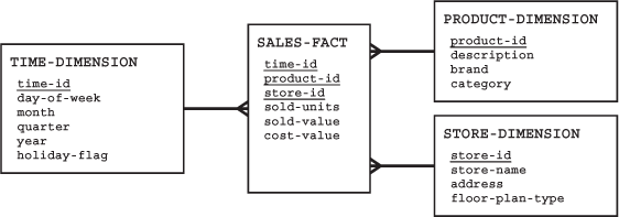
At the centre of the star is a single fact table – in this case the SALES-FACT table. This fact table has a many-to-one relationship with each of the dimension tables, STORE-DIMENSION, PRODUCT-DIMENSION and TIME-DIMENSION.

In this schema, the fact table contains the daily sales totals, that is, the units sold, the cost value and the sale value, for each product in each store. This is as a result of a decision that was made following an analysis of the likely queries that may be made of the data. If it is likely that a user may at some time in the future wish to analyse the distribution of sales throughout a day the time dimension table needs an additional column (say ‘hour’). Decisions about the granularity of the dimensions of the data warehouse are, therefore, very important. Users can only drill down to the lowest level of granularity at which data is stored. Once data has been stored in the data warehouse with the granularity of the time dimension being set as a day, it is impossible to determine the pattern of sales at different times during the day.

There are a number of things to note about this schema. The primary key of the fact table is the combination of the foreign keys that reference the dimension tables. The only non-key columns of the fact table are all numerical. This is important because they are to be subject to statistical analysis. The dimension tables are not normalised – there is a lot of repetition of data. Additionally, the TIME-DIMENSION table has a column called holiday-flag. This enables users to query the data to see what effect holidays have on the sales. The other columns in the time-dimension table allow for analyses that compare sales on Mondays against sales on, say, Tuesdays, January sales against March sales, first quarter sales against third quarter sales, and sales on May Day Bank Holiday 2006 against May Day Bank Holiday 2007. The STORE-DIMENSION table has a floor-plan-type column. This allows analyses that look at the extent to which different store layouts may influence sales. Why are the fruit and vegetables by the entrance and the in-store bakeries diagonally opposite the entrance in most supermarkets?

There are possible variations on the star schema. A snowflake schema introduces a degree of normalisation into the dimensions. A galaxy schema has two or more fact tables that share one or more of the dimensions. The latest versions of SQL have introduced support for OLAP operations with a relational schema, such as a GROUP BY ROLLUP facility.