
companyId   name                 parentCompanyId
----------- -------------------- ---------------
1           Company HQ           NULL
2           Maine HQ             1
3           Tennessee HQ         1
4           Nashville Branch     3
5           Knoxville Branch     3
6           Memphis Branch       3
7           Portland Branch      2
8           Camden Branch        2
You can traverse the data from child to parent fairly easy using the key structures. In the next code, we will write a query to get the children of a given node and add a column to the output that shows the hierarchy. I have commented the code to show what I was doing, but it is fairly straightforward how this code works once you have wrapped your head around it a few times. Recursive CTEs are not always the easiest code to follow:
--getting the children of a row (or ancestors with slight mod to query)
DECLARE @CompanyId int = <set me>;
;WITH companyHierarchy(CompanyId, ParentCompanyId, treelevel, hierarchy)
AS
(
     --gets the top level in hierarchy we want. The hierarchy column
     --will show the row’s place in the hierarchy from this query only
     --not in the overall reality of the row’s place in the table
     SELECT CompanyId, ParentCompanyId,
            1 AS treelevel, CAST(CompanyId AS varchar(max)) as hierarchy
     FROM   Corporate.Company
     WHERE CompanyId=@CompanyId
     UNION ALL
     --joins back to the CTE to recursively retrieve the rows
     --note that treelevel is incremented on each iteration
     SELECT Company.CompanyID, Company.ParentCompanyId,
            treelevel + 1 AS treelevel,
            CONCAT(hierarchy,’’,Company.CompanyId) AS hierarchy
     FROM   Corporate.Company
              INNER JOIN companyHierarchy
                --use to get children
                ON Company.ParentCompanyId= companyHierarchy.CompanyId
                --use to get parents
                --ON Company.CompanyId= companyHierarchy.ParentcompanyId
)
--return results from the CTE, joining to the company data to get the
--company name
SELECT  Company.CompanyID,Company.Name,
        companyHierarchy.treelevel, companyHierarchy.hierarchy
FROM     Corporate.Company
         INNER JOIN companyHierarchy
              ON Company.CompanyId = companyHierarchy.companyId
ORDER BY hierarchy;
Running this code with @companyId = 1, you will get the following:
companyID   name                 treelevel   hierarchy
----------- -------------------- ----------- ----------
1           Company HQ           1           1
2           Maine HQ             2           12
7           Portland Branch      3           127
8           Camden Branch        3           128
3           Tennessee HQ         2           13
4           Nashville Branch     3           134
5           Knoxville Branch     3           135
6           Memphis Branch       3           136
![]() Tip Make a note of the hierarchy output here. This is very similar to the data used by what will be called the “path” method and will show up in the hierarchyId examples as well.
Tip Make a note of the hierarchy output here. This is very similar to the data used by what will be called the “path” method and will show up in the hierarchyId examples as well.
The hierarchy column shows you the position of each of the children of the ’Company HQ’ row, and since this is the only row with a null parentCompanyId, you don’t have to start at the top; you can start in the middle. For example, the ’Tennessee HQ’(@companyId = 3) row would return
companyID   name                 treelevel   hierarchy
----------- -------------------- ----------- -----------
3           Tennessee HQ         1           3
4           Nashville Branch     2           34
5           Knoxville Branch     2           35
6           Memphis Branch       2           36
If you want to get the parents of a row, you need to make just a small change to the code. Instead of looking for rows in the CTE that match the companyId of the parentCompanyId, you look for rows where the parentCompanyId in the CTE matches the companyId. I left in some code with comments:
                --use to get children
                ON company.parentCompanyId= companyHierarchy.companyId
                --use to get parents
                --ON company.CompanyId= companyHierarchy.parentcompanyId
Comment out the first ON, and uncomment the second one:
                --use to get children
                --ON company.parentCompanyId= companyHierarchy.companyId
                --use to get parents
                ON company.CompanyId= companyHierarchy.parentcompanyId
And change @companyId to a row with parents, such as 4. Running this you will get
companyID   name                 treelevel   hierarchy
----------- -------------------- ----------- ----------------------------------
4           Nashville Branch     1           4
3           Tennessee HQ         2           43
1           Company HQ           3           431
The hierarchy column now shows the relationship of the row to the starting point in the query, not its place in the tree. Hence, it seems backward, but thinking back to the breadth-first searching approach, you can see that on each level, the hierarchy columns in all examples have added data for each iteration.
I should also make note of one issue with hierarchies, and that is circular references. We could easily have the following situation occur:
ObjectId    ParentId
----------  ---------
1           3
2           1
3           2
In this case, anyone writing a recursive-type query would get into an infinite loop because every row has a parent, and the cycle never ends. This is particularly dangerous if you limit recursion on a CTE (100 by default, and controlled per statement via the MAXRECURSION query option; set to 0 and no limit is applied) and you stop after MAXRECURSION iterations rather than failing, and hence never noticing.
Graphs (Multiparent Hierarchies)
Querying graphs is a very complex topic that is well beyond the scope of this book and chapter. This section provides a brief overview. There are two types of graph-querying problems that you may come up against:
- Directed: While the node may have more than one parent, there may not exist cycles in the graph. This is common in a graph like a bill of materials/product breakdown. In this case, you can process a slice of the graph from parent to children exactly like a tree. As no item can be a child and a grandparent of the same node.
- Undirected: The far more typical graph. An example of an undirected graph is seen in a representation of actors and movies (not to mention directors, staff, clips, etc.). It is often noted in the problem of “Seven Degrees of Kevin Bacon” whereas Kevin Bacon can be linked to almost anyone in seven steps. He was in a movie with Actor1, who was in a movie with Actor2, who was in a movie with Actor3. And Actor3 may have been in two movies with Actor1 already and so forth. When processing a graph, you have to detect cycles and stop processing.
Let’s look at a bill of materials. Say you have part A, and you have two assemblies that use this part. So the two assemblies are parents of part A. Using an adjacency list embedded in the table with the data, you cannot represent anything other than a tree (we will look at several combinations of object configurations to tweak what your database can model). We split the data from the implementation of the hierarchy. As an example, consider the following schema with parts and assemblies.
First, we create a table for the parts:
CREATE SCHEMA Parts;
GO
CREATE TABLE Parts.Part
(
        PartId   int    NOT NULL CONSTRAINT PKPart PRIMARY KEY,
        PartNumber char(5) NOT NULL CONSTRAINT AKPart UNIQUE,
        Name    varchar(20) NULL
);
Then, we load in some simple data:
INSERT INTO Parts.Part (PartId, PartNumber,Name)
VALUES (1,’00001’,’Screw Package’),(2,’00002’,’Piece of Wood’),
       (3,’00003’,’Tape Package’),(4,’00004’,’Screw and Tape’),
       (5,’00005’,’Wood with Tape’) ,(6,’00006’,’Screw’),(7,’00007’,’Tape’);
Next, we create a table to hold the part containership setup:
CREATE TABLE Parts.Assembly
(
       PartId   int
            CONSTRAINT FKAssembly$contains$PartsPart
                              REFERENCES Parts.Part(PartId),
       ContainsPartId   int
            CONSTRAINT FKAssembly$isContainedBy$PartsPart
                              REFERENCES Parts.Part(PartId),
            CONSTRAINT PKAssembly PRIMARY KEY (PartId, ContainsPartId)
);
First, set up the two packages of screw and tape:
INSERT INTO PARTS.Assembly(PartId,ContainsPartId)
VALUES (1,6),(3,7);
Now, you can load in the data for the Screw and Tape part, by making the part with partId 4 a parent to 1 and 3:
INSERT INTO PARTS.Assembly(PartId,ContainsPartId)
VALUES (4,1),(4,3);
Finally, you can do the same thing for the Wood with Tape part:
INSERT INTO Parts.Assembly(PartId,ContainsPartId)
VALUES (5,2),(5,3);
Now you can take any part in the hierarchy, and use the same recursive CTE-style algorithm and pull out the tree of data you are interested in. In the first go I will get the ’Screw and Tape’ assembly which is PartId=4:
--getting the children of a row (or ancestors with slight mod to query)
DECLARE @PartId int = 4;
;WITH partsHierarchy(PartId, ContainsPartId, treelevel, hierarchy,nameHierarchy)
AS
(
     --gets the top level in hierarchy we want. The hierarchy column
     --will show the row’s place in the hierarchy from this query only
     --not in the overall reality of the row’s place in the table
     SELECT NULL  AS PartId, PartId AS ContainsPartId,
            1 AS treelevel,
            CAST(PartId AS varchar(max)) as hierarchy,
            --added more textual hierarchy for this example
            CAST(Name AS varchar(max)) AS nameHierarchy
     FROM   Parts.Part
     WHERE PartId=@PartId
     UNION ALL
     --joins back to the CTE to recursively retrieve the rows
     --note that treelevel is incremented on each iteration
     SELECT Assembly.PartId, Assembly.ContainsPartId,
            treelevel + 1 as treelevel,
            CONCAT(hierarchy,’’,Assembly.ContainsPartId) AS hierarchy,
            CONCAT(nameHierarchy,’’,Part.Name) AS nameHierarchy
     FROM   Parts.Assembly
                          INNER JOIN Parts.Part
                                ON Assembly.ContainsPartId = Part.PartId
              INNER JOIN partsHierarchy
                ON Assembly.PartId= partsHierarchy.ContainsPartId
)
SELECT PartId, nameHierarchy, hierarchy
FROM partsHierarchy;
This returns
PartId      nameHierarchy                        hierarchy
----------- ------------------------------------ ------------
NULL        Screw and Tape                       4
4           Screw and TapeScrew Package         41
4           Screw and TapeTape Package          43
3           Screw and TapeTape PackageTape     437
1           Screw and TapeScrew PackageScrew   416
Change the variable to 5, and you will see the other part we configured:
PartId      nameHierarchy                        hierarchy
----------- ------------------------------------ ------------
NULL        Wood with Tape                       5
5           Wood with TapePiece of Wood         52
5           Wood with TapeTape Package          53
3           Wood with TapeTape PackageTape     537
As you can see, the tape package is repeated from the other part configuration. I won’t cover dealing with cycles in graphs in the text (it will be a part of the extended examples), but the biggest issue when dealing with cyclical graphs is making sure that you don’t double count data because of the cardinality of the relationship.
Implementing the Hierarchy Using the hierarchyId Type
In addition to the fairly standard adjacency list implementation, there is also a datatype called hierarchyId that is a proprietary CLR-based datatype that can be used to do some of the heavy lifting of dealing with hierarchies. It has some definite benefits in that it makes queries on hierarchies fairly easier, but it has some difficulties as well.
The primary downside to the hierarchyId datatype is that it is not as simple to work with for some of the basic tasks as is the self-referencing column. Putting data in this table will not be as easy as it was for that method (recall all of the data was inserted in a single statement, which will not be possible for the hierarchyId solution, unless you have already calculated the path). However, on the bright side, the types of things that are harder with using a self-referencing column will be notably easier, but some of the hierarchyId operations are not what you would consider natural at all.
As an example, I will set up an alternate company table named corporate2 where I will implement the same table as in the previous example using hierarchyId instead of the adjacency list. Note the addition of a calculated column that indicates the level in the hierarchy, which will be used by the internals to support breadth-first processing. The surrogate key CompanyId is not clustered to allow for a future index. If you do a large amount of fetches by the primary key, you may want to implement the hierarchy as a separate table.
CREATE TABLE Corporate.CompanyAlternate
(
    CompanyOrgNode hierarchyId not null
                 CONSTRAINT AKCompanyAlternate UNIQUE,
    CompanyId   int CONSTRAINT PKCompanyAlternate PRIMARY KEY NONCLUSTERED,
    Name        varchar(20) CONSTRAINT AKCompanyAlternate_name UNIQUE,
    OrganizationLevel AS CompanyOrgNode.GetLevel() PERSISTED
);
You will also want to add an index that includes the level and hierarchyId node. Without the calculated column and index (which are not at all intuitively obvious), the performance of this method will degrade rapidly as your hierarchy grows:
CREATE CLUSTERED INDEX Org_Breadth_First
         ON Corporate.CompanyAlternate(OrganizationLevel,CompanyOrgNode);
To insert a root node (with no parent), you use the GetRoot() method of the hierarchyId type without assigning it to a variable:
INSERT Corporate.CompanyAlternate (CompanyOrgNode, CompanyId, Name)
VALUES (hierarchyid::GetRoot(), 1, ’Company HQ’);
To insert child nodes, you need to get a reference to the parentCompanyOrgNode that you want to add, then find its child with the largest companyOrgNode value, and finally, use the getDecendant() method of the companyOrgNode to have it generate the new value. I have encapsulated it into the following procedure (based on the procedure in the tutorials from Books Online, with some additions to support root nodes and single-threaded inserts, to avoid deadlocks and/or unique key violations), with comments to explain how the code works:
CREATE PROCEDURE Corporate. CompanyAlternate$Insert(@CompanyId int, @ParentCompanyId int,
                                           @Name varchar(20))
AS
BEGIN
   SET NOCOUNT ON
   --the last child will be used when generating the next node,
   --and the parent is used to set the parent in the insert
   DECLARE  @lastChildofParentOrgNode hierarchyid,
            @parentCompanyOrgNode hierarchyid;
   IF @ParentCompanyId IS NOT NULL
     BEGIN
        SET @ParentCompanyOrgNode =
                            (  SELECT CompanyOrgNode
                               FROM   Corporate. CompanyAlternate
                               WHERE  CompanyID = @ParentCompanyId)
         IF  @parentCompanyOrgNode IS NULL
           BEGIN
                THROW 50000, ’Invalid parentCompanyId passed in’,1;
                RETURN -100;
           END;
     END;
   BEGIN TRANSACTION;
      --get the last child of the parent you passed in if one exists
      SELECT @lastChildofParentOrgNode = MAX(CompanyOrgNode)
      FROM Corporate.CompanyAlternate (UPDLOCK) --compatible with shared, but blocks
                                       --other connections trying to get an UPDLOCK
      WHERE CompanyOrgNode.GetAncestor(1) = @parentCompanyOrgNode ;
      --getDecendant will give you the next node that is greater than
      --the one passed in.  Since the value was the max in the table, the
      --getDescendant Method returns the next one
      INSERT Corporate.CompanyAlternate  (CompanyOrgNode, CompanyId, Name)
             --the coalesce puts the row as a NULL this will be a root node
             --invalid ParentCompanyId values were tossed out earlier
      SELECT COALESCE(@parentCompanyOrgNode.GetDescendant(
                   @lastChildofParentOrgNode, NULL),hierarchyid::GetRoot())
                  ,@CompanyId, @Name;
   COMMIT;
END;
Now, create the rest of the rows:
--exec Corporate.CompanyAlternate$insert @CompanyId = 1, @parentCompanyId = NULL,
--                               @Name = ’Company HQ’; --already created
exec Corporate.CompanyAlternate$insert @CompanyId = 2, @ParentCompanyId = 1,
                                 @Name = ’Maine HQ’;
exec Corporate.CompanyAlternate$insert @CompanyId = 3, @ParentCompanyId = 1,
                                 @Name = ’Tennessee HQ’;
exec Corporate.CompanyAlternate$insert @CompanyId = 4, @ParentCompanyId = 3,
                                 @Name = ’Knoxville Branch’;
exec Corporate.CompanyAlternate$insert @CompanyId = 5, @ParentCompanyId = 3,
                                 @Name = ’Memphis Branch’;
exec Corporate.CompanyAlternate$insert @CompanyId = 6, @ParentCompanyId = 2,
                                 @Name = ’Portland Branch’;
exec Corporate.CompanyAlternate$insert @CompanyId = 7, @ParentCompanyId = 2,
                                 @Name = ’Camden Branch’;
You can see the data in its raw format here:
SELECT CompanyOrgNode, CompanyId, Name
FROM   Corporate.CompanyAlternate
ORDER  BY CompanyId;
This returns a fairly uninteresting result set, particularly since the companyOrgNode value is useless in this untranslated format:
companyOrgNode      companyId   name
------------------------------- ------------------
0x                  1           Company HQ
0x58                2           Maine HQ
0x68                3           Tennessee HQ
0x6AC0              4           Knoxville Branch
0x6B40              5           Nashville Branch
0x6BC0              6           Memphis Branch
0x5AC0              7           Portland Branch
0x5B40              8           Camden Branch
But this is not the most interesting way to view the data. The type includes methods to get the level, the hierarchy, and more:
SELECT CompanyId, OrganizationLevel,
       Name, CompanyOrgNode.ToString() as Hierarchy
FROM   Corporate.CompanyAlternate
ORDER  BY Hierarchy;
This can be really useful in queries:
companyId   OrganizationLevel  name                 hierarchy
----------- ------------------ -------------------- -------------
1           0                  Company HQ           /
2           1                  Maine HQ             /1/
6           2                  Portland Branch      /1/1/
7           2                  Camden Branch        /1/2/
3           1                  Tennessee HQ         /2/
4           2                  Knoxville Branch     /2/1/
5           2                  Memphis Branch       /2/2/
Getting all of the children of a node is far easier than it was with the previous method. The hierarchyId type has an IsDecendantOf() method you can use. For example, to get the children of companyId = 3, use the following:
DECLARE @CompanyId int = 3;
SELECT Target.CompanyId, Target.Name, Target.CompanyOrgNode.ToString() AS Hierarchy
FROM   Corporate.CompanyAlternate AS Target
               JOIN Corporate.CompanyAlternate AS SearchFor
                       ON SearchFor.CompanyId = @CompanyId
                          and Target.CompanyOrgNode.IsDescendantOf
                                                 (SearchFor.CompanyOrgNode) = 1;
This returns
CompanyId   Name                 Hierarchy
----------- -------------------- ------------
3           Tennessee HQ         /2/
4           Knoxville Branch     /2/1/
5           Memphis Branch       /2/2/
What is nice is that you can see in the hierarchy the row’s position in the overall hierarchy without losing how it fits into the current results. In the opposite direction, getting the parents of a row isn’t much more difficult. You basically just switch the position of the SearchFor and the Target in the ON clause:
DECLARE @CompanyId int = 3;
SELECT Target.CompanyId, Target.Name, Target.CompanyOrgNode.ToString() AS Hierarchy
FROM   Corporate.CompanyAlternate AS Target
               JOIN Corporate.CompanyAlternate AS SearchFor
                       ON SearchFor.CompanyId = @CompanyId
                          and SearchFor.CompanyOrgNode.IsDescendantOf
                                                 (Target.CompanyOrgNode) = 1;
This returns
companyId   name                 hierarchy
----------- -------------------- ----------
1           Company HQ           /
3           Tennessee HQ         /2/
This query is a bit easier to understand than the recursive CTEs we previously needed to work with. And this is not all that the datatype gives you. This chapter and section are meant to introduce topics, not be a complete reference. Check out Books Online for a full reference to hierarchyId.
However, while some of the usage is easier, using hierarchyId has several negatives, most particularly when moving a node from one parent to another. There is a reparent method for hierarchyId, but it only works on one node at a time. To reparent a row (if, say, Oliver is now reporting to Cindy rather than Bobby), you will have to reparent all of the people that work for Oliver as well. In the adjacency model, simply moving modifying one row can move all rows at once.
Alternative Methods/Query Optimizations
Dealing with hierarchies in relational data has long been a well-trod topic. As such, a lot has been written on the subject of hierarchies and quite a few other techniques that have been implemented. In this section, I will give an overview of three other ways of dealing with hierarchies that have been and will continue to be used in designs:
- Path technique: In this method, which is similar internally to using hierarchyId, (though without the methods on a datatype to work with,) you store the path from the child to the parent in a formatted text string.
- Nested sets: Use the position in the tree to allow you to get children or parents of a row very quickly.
- Kimball helper table: Basically, this stores a row for every single path from parent to child. It’s great for reads but tough to maintain and was developed for read-only situations, like read-only databases.
Each of these methods has benefits. Each is more difficult to maintain than a simple adjacency model or even the hierarchyId solution but can offer benefits in different situations. In the following sections, I am going to give a brief illustrative overview of each.
Path Technique
The path technique is pretty much the manual version of the hierarchyId method. In it, you store the path from the parent to the child. Using our hierarchy that we have used so far, to implement the path method we could use the set of data in Figure 8-7. Note that each of the tags in the hierarchy will use the surrogate key for the key values in the path, so it will be essential that the value is immutable. In Figure 8-7, I have included a diagram of the hierarchy implemented with the path value set for our design.

Figure 8-7. Sample hierarchy diagram with values for the path technique
With the path in this manner, you can find all of the children of a row using the path in a like expression. For example, to get the children of the Main HQ node, you can use a WHERE clause such as WHERE Path LIKE ’12\%’ to get the children, and the path to the parents is directly in the path too. So the parents of the Portland Branch, whose path is ’124’, are ’12’ and ’1’.
One of the great things about the path method is that it readily uses indexes, because most of the queries you will make will use the left side of a string. So up to SQL Server 2014, as long as your path could stay below 900 bytes, your performance is generally awesome. In 2016, the max keylength has been increased to 1,700 bytes, which is great, but if your paths are this long, you will only end up with four keys per page, which is not going to give amazing performance (indexes will be covered in detail in Chapter 10).
One of the more clever methods of dealing with hierarchies was created in 1992 by Michael J. Kamfonas. It was introduced in an article named “Recursive Hierarchies: The Relational Taboo!” in The Relational Journal, October/November 1992. It is also a favorite method of Joe Celko, who has written a book about hierarchies named Joe Celko’s Trees and Hierarchies in SQL for Smarties (Morgan Kaufmann, 2004); check it out (now in its second edition, 2012) for further reading about this and other types of hierarchies.
The basics of the method is that you organize the tree by including pointers to the left and right of the current node, enabling you to do math to determine the position of an item in the tree. Again, going back to our company hierarchy, the structure would be as shown in Figure 8-8.
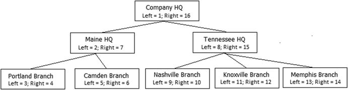
Figure 8-8. Sample hierarchy diagram with values for the nested sets technique
This has the value of now being able to determine children and parents of a node very quickly. To find the children of Maine HQ, you would say WHERE Left > 2 and Right < 7. No matter how deep the hierarchy, there is no traversing the hierarchy at all, just simple integer comparisons. To find the parents of Maine HQ, you simply need to look for the case WHERE Left < 2 and Right > 7.
Adding a node has a rather negative effect of needing to update all rows to the right of the node, increasing their Right value, since every single row is a part of the structure. Deleting a node will require decrementing the Right value. Even reparenting becomes a math problem, just requiring you to update the linking pointers. Probably the biggest downside is that it is not a very natural way to work with the data, since you don’t have a link directly from parent to child to navigate.
Finally, in a method that is going to be the most complex to manage (but in most cases, the fastest to query), you can use a method that Ralph Kimball created for dealing with hierarchies, particularly in a data warehousing/read-intensive setting, but it could be useful in an OLTP setting if the hierarchy is fairly stable. Going back to our adjacency list implementation, shown in Figure 8-9, assume we already have this implemented in SQL.

Figure 8-9. Sample hierarchy diagram with values for the adjacency list technique repeated for the Kimball helper table method
To implement this method, you will use a table of data that describes the hierarchy with one row per parent-to-child relationship, for every level of the hierarchy. So there would be a row for Company HQ to Maine HQ, Company HQ to Portland Branch, etc. The helper table provides the details about distance from parent, if it is a root node or a leaf node. So, for the leftmost four items (1, 2, 4, 5) in the tree, we would get the following table:

The power of this technique is that now you can simply ask for all children of 1 by looking for WHERE ParentId = 1, or you can look for direct descendents of 2 by saying WHERE ParentId = 2 and Distance = 1. And you can look for all leaf notes of the parent by querying WHERE ParentId = 1 and ChildLeafNode = 1. The code to implement this structure is basically a slightly modified version of the recursive CTE used in our first hierarchy example. It may take a few minutes to rebuild for a million nodes.
The obvious downfall of this method is simple. It is somewhat costly to maintain if the structure is modified frequently. To be honest, Kimball’s purpose for the method was to optimize relational usage of hierarchies in the data warehouse, which is maintained by ETL. For this sort of purpose, this method should be the quickest, because all queries will be almost completely based on simple relational queries. Of all of the methods, this one will be the most natural for users, while being the less desirable to the team that has to maintain the data.
Images, Documents, and Other Files, Oh My!
Storing large binary objects, such as PDFs, images, and really any kind of object you might find in your Windows file system, is generally not the historic domain of the relational database. As time has passed, however, it is becoming more and more commonplace.
When discussing how to store large objects in SQL Server, generally speaking this would be in reference to data that is (obviously) large but usually in some form of binary format that is not naturally modified using common T-SQL statements, for example, a picture or a formatted document. Most of the time, this is not considering simple text data or even formatted, semistructured text, or even highly structured text such as XML. SQL Server has an XML type for storing XML data (including the ability to index fields in the XML document), and it also has varchar(max)/nvarchar(max) types for storing very large “plain” text data. Of course, sometimes, you will want to store text data in the form of a Windows text file to allow users to manage the data naturally. When deciding on a way to store binary data in SQL Server, there are two broadly characterizable ways that are available:
In early editions of this book, the question was pretty easy to answer indeed. Almost always, the most reasonable solution was to store files in the file system and just store a reference to the data in a varchar column. In SQL Server 2008, Microsoft implemented a type of binary storage called a filestream, which allows binary data to be stored in the file system as actual files, which makes accessing this data from a client much faster than if it were stored in a binary column in SQL Server. In SQL Server 2012, the picture improved even more to give you a method to store any file data in the server that gives you access to the data using what looks like a typical network share. In all cases, you can deal with the data in T-SQL as before, and even that may be improved, though you cannot do partial writes to the values like you can in a basic varbinary(max) column.
Over the course of time, the picture hasn’t changed terribly. I generally separate the choice between the two possible ways to store binaries into one primary simple reason to choose one or the other: transactional integrity. If you require transaction integrity, you use SQL Server’s storage engine, regardless of the cost you may incur. If transaction integrity isn’t tremendously important, you probably will want to use the file system. For example, if you are just storing an image that a user could go out and edit, leaving it with the same name, the file system is perfectly natural. Performance is a consideration, but if you need performance, you could write the data to the storage engine first and then regularly refresh the image to the file system and use it from a cache.
If you are going to store large objects in SQL Server, you will usually want to use filestream, particularly if your files are of fairly large size. It is suggested that you definitely consider filestream if your binary objects will be greater than 1MB, but recommendations change over time. Setting up filestream access is pretty easy; first, you enable filestream access for the server. For details on this process, check the Books Online topic “Enable and Configure FILESTREAM” (https://msdn.microsoft.com/en-us/library/cc645923.aspx). The basics to enable filestream (if you did not already do this during the process of installation) are to go to SQL Server Configuration Manager and choose the SQL Server Instance in SQL Server Services. Open the properties, and choose the FILESTREAM tab, as shown in Figure 8-10.

Figure 8-10. Configuring the server for filestream access
The Windows share name will be used to access filestream data via the API, as well as using a filetable later in this chapter. Later in this section, there will be additional configurations based on how the filestream data will be accessed. Start by enabling filestream access for the server using sp_configure filestream_access_level of either 1 (T-SQL access) or 2 (T-SQL and Win32 access). We will be using both methods, so I will use the latter:
EXEC sp_configure filestream_access_level 2;
RECONFIGURE;
Next, we create a sample database (instead of using pretty much any database as we have for the rest of this chapter):
CREATE DATABASE FileStorageDemo; --uses basic defaults from model database
GO
USE FileStorageDemo;
GO
--will cover filegroups more in the Chapter 10 on structures
ALTER DATABASE FileStorageDemo ADD
        FILEGROUP FilestreamData CONTAINS FILESTREAM;
![]() Tip There are caveats with using filestream data in a database that also needs to use snapshot isolation level or that implements the READ_COMMITTED_SNAPSHOT database option. Go to SET TRANSACTION ISOLATION LEVEL statement (covered in Chapter 11) documentation here https://msdn.microsoft.com/en-us/library/ms173763.aspx for more information.
Tip There are caveats with using filestream data in a database that also needs to use snapshot isolation level or that implements the READ_COMMITTED_SNAPSHOT database option. Go to SET TRANSACTION ISOLATION LEVEL statement (covered in Chapter 11) documentation here https://msdn.microsoft.com/en-us/library/ms173763.aspx for more information.
Next, add a “file” to the database that is actually a directory for the filestream files (note that the directory should not exist before executing the following statement, but the directory, in this case, c:sql, must exist or you will receive an error):
ALTER DATABASE FileStorageDemo ADD FILE (
       NAME = FilestreamDataFile1,
       FILENAME = ’c:sqlfilestream’) --directory cannot yet exist and SQL account must have
                                        --access to drive.
TO FILEGROUP FilestreamData;
Now, you can create a table and include a varbinary(max) column with the keyword FILESTREAM after the datatype declaration. Note, too, that we need a unique identifier column with the ROWGUIDCOL property that is used by some of the system processes as a kind of special surrogate key.
CREATE SCHEMA Demo;
GO
CREATE TABLE Demo.TestSimpleFileStream
(
        TestSimpleFilestreamId INT NOT NULL
                      CONSTRAINT PKTestSimpleFileStream PRIMARY KEY,
        FileStreamColumn VARBINARY(MAX) FILESTREAM NULL,
        RowGuid uniqueidentifier NOT NULL ROWGUIDCOL DEFAULT (NEWID())
                      CONSTRAINT AKTestSimpleFileStream_RowGuid UNIQUE
)       FILESTREAM_ON FilestreamData;
It is as simple as that. You can use the data exactly like it is in SQL Server, as you can create the data using a simple query:
INSERT INTO Demo.TestSimpleFileStream(TestSimpleFilestreamId,FileStreamColumn)
SELECT 1, CAST(’This is an exciting example’ AS varbinary(max));
and see it using a typical SELECT:
SELECT TestSimpleFilestreamId,FileStreamColumn,
       CAST(FileStreamColumn AS varchar(40)) AS FileStreamText
FROM   Demo.TestSimpleFilestream;
I won’t go any deeper into filestream manipulation here, because all of the more interesting bits of the technology from here are external to SQL Server in API code, which is well beyond the purpose of this section, which is to show you the basics of setting up the filestream column in your structures.
In SQL Server 2012, we got a new feature for storing binary files called a filetable. A filetable is a special type of table that you can access using T-SQL or directly from the file system using the share we set up earlier in this section, named MSSQLSERVER. One of the nice things for us is that we will actually be able to see the file that we create in a very natural manner that is accessible from Windows Explorer.
Enable and set up filetable style filestream in the database as follows:
ALTER DATABASE FileStorageDemo
        SET FILESTREAM (NON_TRANSACTED_ACCESS = FULL,
                         DIRECTORY_NAME = N’ProSQLServerDBDesign’);
The setting NON_TRANSACTED_ACCESS lets you set whether or not users can change data when accessing the data as a Windows share, such as opening a document in Word. The changes are not transactionally safe, so data stored in a filetable is not as safe as using a simple varbinary(max) or even one using the filestream attribute. It behaves pretty much like data on any file server, except that it will be backed up with the database, and you can easily associate a file with other data in the server using common relational constructs. The DIRECTORY_NAME parameter is there to add to the path you will access the data (this will be demonstrated later in this section).
The syntax for creating the filetable is pretty simple:
CREATE TABLE Demo.FileTableTest AS FILETABLE
  WITH (
        FILETABLE_DIRECTORY = ’FileTableTest’,
        FILETABLE_COLLATE_FILENAME = database_default
        );
The FILETABLE_DIRECTORY is the final part of the path for access, and the FILETABLE_COLLATE_FILENAME determines the collation that the filenames will be treated as. It must be case insensitive, because Windows directories are case insensitive. I won’t go in depth with all of the columns and settings, but suffice it to say that the filetable is based on a fixed table schema, and you can access it much like a common table. There are two types of rows, directories, and files. Creating a directory is easy. For example, if you wanted to create a directory for Project 1:
INSERT INTO Demo.FiletableTest(name, is_directory)
VALUES ( ’Project 1’, 1);
Then, you can view this data in the table:
SELECT stream_id, file_stream, name
FROM   Demo.FileTableTest
WHERE  name = ’Project 1’;
This will return (though with a different stream_id)
stream_id                            file_stream                         name
-------------- ------------9BCB8987-1DB4-E011-87C8-000C29992276          Project 1
stream_id is a unique key that you can relate to with your other tables, allowing you to simply present the user with a “bucket” for storing data. Note that the primary key of the table is the path_locator hierarchyId, but this is a changeable value. The stream_id value shouldn’t ever change, though the file or directory could be moved. Before we go check it out in Windows, let’s add a file to the directory. We will create a simple text file, with a small amount of text:
INSERT INTO Demo.FiletableTest(name, is_directory, file_stream)
VALUES ( ’Test.Txt’, 0, CAST(’This is some text’ AS varbinary(max)));
Then, we can move the file to the directory we just created using the path_locator hierarchyId functionality. (The directory hierarchy is built on hierarchyId. In the downloads for hierarchies from the earlier section, you can see more details of the methods you can use here as well as your own hierarchies.)
UPDATE Demo.FiletableTest
SET    path_locator = path_locator.GetReparentedValue( path_locator.GetAncestor(1),
       (SELECT path_locator FROM Demo.FiletableTest
            WHERE name = ’Project 1’
                  AND parent_path_locator IS NULL
                  AND is_directory = 1))
WHERE name = ’Test.Txt’;
Now, go to the share that you have set up and view the directory in Windows. Using the function FileTableRootPath(), you can get the filetable path for the database; in my case, the name of my VM is WIN-8F59BO5AP7D, so the share is \WIN-8F59BO5AP7DMSSQLSERVERProSQLServerDBDesign, which is my computer’s name, the MSSQLSERVER we set up in Configuration Manager, and ProSQLServerDBDesign from the ALTER DATABASE statement turning on filestream.
Now, concatenating the root to the path for the directory, which can be retrieved from the file_stream column (yes, the value you see when querying it is NULL, which is a bit confusing). Now, execute this:
SELECT  CONCAT(FileTableRootPath(),
                            file_stream.GetFileNamespacePath()) AS FilePath
FROM    Demo.FileTableTest
WHERE   name = ’Project 1’
  AND   parent_path_locator is NULL
  AND   is_directory = 1;
This returns the following:
FilePath
-----------------------------------------------------------------------------
\WIN-8F59BO5AP7DMSSQLSERVERProSQLServerDBDesignFileTableTestProject 1
You can then enter this into Explorer to see something like what’s shown in Figure 8-11 (assuming you have everything configured correctly, of course). Note that security for the Windows share is the same as for the filetable through T-SQL, which you administer the same as with any regular table, and you may need to set up your firewall to allow access as well.
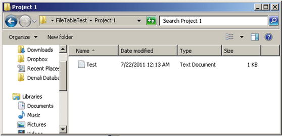
Figure 8-11. Filetable directory opened in Windows Explorer
From here, I would suggest you drop a few files in the directory from your local drive and check out the metadata for your files in your newly created filetable. It has a lot of possibilities. I will touch more on security in Chapter 9, but the basics are that security is based on Windows Authentication as you have it set up in SQL Server on the table, just like any other table.
![]() Note If you try to use Notepad to access the text file on the same server as the share is located, you will receive an error due to the way Notepad accesses files locally. Accessing the file from a remote location using Notepad will work fine.
Note If you try to use Notepad to access the text file on the same server as the share is located, you will receive an error due to the way Notepad accesses files locally. Accessing the file from a remote location using Notepad will work fine.
I won’t spend any more time covering the particulars of implementing with filetables. Essentially, with very little trouble, even a fairly basic programmer could provide a directory per client to allow the user to navigate to the directory and get the customer’s associated files. And the files can be backed up with the normal backup operations. You don’t have any row-level security over access, so if you need more security, you may need a table per security needs, which may not be optimum for more than a few use cases.
So, mechanics aside, consider the four various methods of storing binary data in SQL tables:
- Store a UNC path in a simple character column
- Store the binary data in a simple varbinary(max) column
- Store the binary data in a varbinary(max) using the filestream type
- Store the binary data using a filetable
![]() Tip There is one other type of method of storing large binary values using what is called the Remote BLOB Store (RBS) API. It allows you to use an external storage device to store and manage the images. It is not a typical case, though it will definitely be of interest to people building high-end solutions needing to store blobs on an external device. For more information, see: https://msdn.microsoft.com/en-us/library/gg638709.aspx.
Tip There is one other type of method of storing large binary values using what is called the Remote BLOB Store (RBS) API. It allows you to use an external storage device to store and manage the images. It is not a typical case, though it will definitely be of interest to people building high-end solutions needing to store blobs on an external device. For more information, see: https://msdn.microsoft.com/en-us/library/gg638709.aspx.
Each of these methods has some merit, and I will discuss the pros and cons in the following list. Like with any newer, seemingly easier technology, a filetable does feel like it might take the nod for a lot of upcoming uses, but definitely consider the other possibilities when evaluating your needs in the future.
- Transactional integrity: Guaranteeing that the image is stored and remains stored is far easier if it is managed by the storage engine, either as a filestream or as a binary value, than if you store the filename and path and have an external application manage the files. A filetable could be used to maintain transactional integrity, but to do so, you will need to disallow nontransaction modifications, which will then limit how much easier it is to work with.
- Consistent backup of image and data: Knowing that the files and the data are in sync is related to transactional integrity. Storing the data in the database, either as a binary columnar value or as a filestream/filetable, ensures that the binary values are backed up with the other database objects. Of course, this can cause your database size to grow very large, so it can be handy to use partial backups of just the data and not the images at times. Filegroups can be restored individually as well, but be careful not to give up integrity for faster backups if the business doesn’t expect it.
- Size: For sheer speed of manipulation, for the typical object size less than 1MB, Books Online suggests using storage in a varchar(max). If objects are going to be more than 2GB, you must use one of the filestream storage types.
- API: Which API is the client using? If the API does not support using the filestream type, you should definitely give it a pass. A filetable will let you treat the file pretty much like it was on any network share, but if you need the file modification to occur along with other changes as a transaction, you will need to use the filestream API.
- Utilization: How will the data be used? If it is used very frequently, then you would choose either filestream/filetable or file system storage. This could particularly be true for files that need to be read-only. Filetable is a pretty nice way to allow the client to view a file in a very natural manner.
- Location of files: Filestream filegroups are located on the same server as the relational files. You cannot specify a UNC path to store the data (as it needs control over the directories to provide integrity). For filestream column use, the data, just like a normal filegroup, must be transactionally safe for utilization.
- Encryption: Encryption is not supported on the data store in filestream filegroups, even when transparent data encryption (TDE) is enabled.
- Security: If the image’s integrity is important to the business process (such as the photo on a security badge that’s displayed to a security guard when a badge is swiped), it’s worth it to pay the extra price for storing the data in the database, where it’s much harder to make a change. (Modifying an image manually in T-SQL is a tremendous chore indeed.) A filetable also has a disadvantage in that implementing row-level security (discussed in Chapter 9 in more detail) using views would not be possible, whereas when using a filestream-based column, you are basically using the data in a SQL-esque manner until you access the file.
For three quick examples, consider a movie rental database (online these days, naturally). In one table, we have a MovieRentalPackage table that represents a particular packaging of a movie for rental. Because this is just the picture of a movie, it is a perfectly valid choice to store a path to the data. This data will simply be used to present electronic browsing of the store’s stock, so if it turns out to not work one time, that is not a big issue. Have a column for the PictureUrl that is varchar(200), as shown in Figure 8-12.

Figure 8-12. MovieRentalPackage table with PictureUrl datatype set as a path to a file
This path might even be on an Internet source where the filename is an HTTP:// address and be located in a web server’s image cache, and could be replicated to other web servers. The path may or may not be stored as a full UNC location; it really would depend on your infrastructure needs. The goal will be, when the page is fetching data from the server, to be able to build a bit of HTML such as this to get the picture that you would display for the movie’s catalog entry:
SELECT ’<img src = "’ + MovieRentalPackage.PictureUrl + ’">’, ...
FROM    Movies.MovieRentalPackage
WHERE   MovieId = @MovieId;
If this data were stored in the database as a binary format, it would need to be materialized onto disk as a file first and then used in the page, which is going to be far slower than doing it this way, no matter what your architecture. This is probably not a case where you would want to do this or go through the hoops necessary for filestream access, since transactionally speaking, if the picture link is broken, it would not invalidate the other data, and it is probably not very important. Plus, you will probably want to access this file directly, making the main web screens very fast and easy to code.
An alternative example might be accounts and associated users (see Figure 8-13). To fight fraud, a movie rental chain may decide to start taking digital photos of customers and comparing the photos to the customers whenever they rent an item. This data is far more important from a security standpoint and has privacy implications. For this, I’ll use a varbinary(max) for the person’s picture in the database.

Figure 8-13. Customer table with picture stored as data in the table
At this point, assume you have definitely decided that transactional integrity is necessary and that you want to retrieve the data directly from the server. The next thing to decide is whether to employ filestreams. The big question with regard to this decision is whether your API supports filestreams. If so, this would likely be a very good place to make use of them. Size could play a part in the choice too, though security pictures could likely be less than 1MB anyhow.
Overall, speed probably isn’t a big deal, and even if you needed to take the binary bits and stream them from SQL Server’s normal storage into a file, it would probably still perform well enough since only one image needs to be fetched at a time, and performance will be adequate as long as the image displays before the rental transaction is completed. Don’t get me wrong; the varbinary(max) types aren’t that slow, but performance would be acceptable for these purposes even if they were.
Finally, consider if you wanted to implement a customer file system to store scanned images pertaining to the customer. Not enough significance is given to the data to require it to be managed in a structured manner, but they simply want to be able to create a directory to hold scanned data. The data does need to be kept in sync with the rest of the database. So, you could extend your table to include a filetable (AccountFileDirectory in Figure 8-14, with stream_id modeled as primary key; even though it is technically a unique constraint in implementation, you can reference an alternate key).

Figure 8-14. Account model extended with an AccountFileDirectory
In this manner, you have included a directory for the account’s files that can be treated like a typical file structure but will be securely located with the account information. This not only will be very usable for the programmer and user alike but will also give you the security of knowing the data is backed up with the account files and treated in the same manner as the account information.
Designing is often discussed as an art form, and that is what this topic is about. When designing a set of tables to represent some real-world activity, how specific should your tables be? For example, if you were designing a database to store information about camp activities, it might be tempting to have an individual table for the archery class, another for the swimming class, and so on, modeling with great detail the activities of each camp activity. If there were 50 activities at the camp, you might have 50 tables, plus a bunch of other tables to tie these 50 together. In the end though, while these tables may not look exactly the same, you would start to notice that every table is used for basically the same thing: assign an instructor, sign up kids to attend, add a description, and so forth. Rather than the system being about each activity, requiring you to model each of the different activities as being different from one another, what you would truly need to do is model the abstraction of a camp activity. On the other hand, while the primary focus of the design would be the management of the activity, you might discover that some extended information is needed about some or all of the classes. Generalization is about making objects as general as possible, employing a pattern like subclassing to tune in the best possible solution.
In the end, the goal is to consider where you can combine foundationally similar tables into a single table, particularly when multiple tables are constantly being treated as one, as you would have to do with the 50 camp activity tables, particularly to make sure kids weren’t signing up their friends for every other session just to be funny.
During design, it is useful to look for similarities in utilization, columns, and so on, and consider collapsing multiple tables into one, ending up with a generalization/abstraction of what is truly needed to be modeled. Clearly, however, the biggest problem here is that sometimes you do need to store different information about some of the things your original tables were modeling. In our example, if you needed special information about the snorkeling class, you might lose that if you just created one activity abstraction, and heaven knows the goal is not to end up with a table with 200 columns all prefixed with what ought to have been a table in the first place (or even worse, one general-purpose bucket of a table with a varchar(max) column where all of the desired information is shoveled into).
In those cases, you can consider using a subclassed entity for certain entities. Take the camp activity model. You could include the generalized table for the generic CampActivity, in which you would associate students and teachers who don’t need special training, and in the subclassed tables, you would include specific information about the snorkeling and archery classes, likely along with the teachers who meet specific criteria (in unshown related tables), as shown in Figure 8-15.

Figure 8-15. Extending generalized entity with specific details as required
As a coded example, we will look at a home inventory system. Suppose we have a client who wants to create an inventory of the various types of stuff in their house, or at least everything valuable, for insurance purposes. So, should we simply design a table for each type of item? That seems like too much trouble, because for almost everything the client will simply have a description, picture, value, and a receipt. On the other hand, a single table, generalizing all of the items in the client’s house down to a single list, seems like it might not be enough for items that they need specific information about, like appraisals and serial numbers. For example, some jewelry probably ought to be appraised and have the appraisal listed. Electronics and appliances ought to have brand, model, and, alternatively, serial numbers captured. So the goal is to generalize a design to the level where the client has a basic list of the home inventory, but can also print a list of jewelry alone with extra detail or print a list of electronics with their identifying information.
So we implement the database as such. First, we create the generic table that holds generic item descriptions:
CREATE SCHEMA Inventory;
GO
CREATE TABLE Inventory.Item
(
        ItemId  int NOT NULL IDENTITY CONSTRAINT PKItem PRIMARY KEY,
        Name    varchar(30) NOT NULL CONSTRAINT AKItemName UNIQUE,
        Type    varchar(15) NOT NULL,
        Color   varchar(15) NOT NULL,
        Description varchar(100) NOT NULL,
        ApproximateValue  numeric(12,2) NULL,
        ReceiptImage   varbinary(max) NULL,
        PhotographicImage varbinary(max) NULL
);
As you can see, I included two columns for holding an image of the receipt and a picture of the item. As discussed in the previous section, you might want to use a filetable construct to just allow various electronic items to be associated with this data, but it would probably be sufficient to simply have a picture of the receipt and the item minimally attached to the row for easy use. In the sample data, I always load the varbinary data with a simple hex value of 0x001 as a placeholder:
INSERT INTO Inventory.Item
VALUES (’Den Couch’,’Furniture’,’Blue’,’Blue plaid couch, seats 4’,450.00,0x001,0x001),
       (’Den Ottoman’,’Furniture’,’Blue’,’Blue plaid ottoman that goes with couch’,
         150.00,0x001,0x001),
       (’40 Inch Sorny TV’,’Electronics’,’Black’,
        ’40 Inch Sorny TV, Model R2D12, Serial Number XD49292’,
         800,0x001,0x001),
        (’29 Inch JQC TV’,’Electronics’,’Black’,’29 Inch JQC CRTVX29 TV’,800,0x001,0x001),
        (’Mom’’s Pearl Necklace’,’Jewelery’,’White’,
         ’Appraised for $1300 in June of 2003. 30 inch necklace, was Mom’’s’,
         1300,0x001,0x001);
Checking out the data using the following query:
SELECT Name, Type, Description
FROM   Inventory.Item;
we see that we have a good little system, though data isn’t organized how we really need it to be, because in realistic usage, we will probably need some of the specific data from the descriptions to be easier to access:
Name                           Type            Description
------------------------------ --------------- -------------------------------------
Den Couch                      Furniture       Blue plaid couch, seats 4
Den Ottoman                    Furniture       Blue plaid ottoman that goes with ...
40 Inch Sorny TV               Electronics     40 Inch Sorny TV, Model R2D12, Ser...
29 Inch JQC TV                 Electronics     29 Inch JQC CRTVX29 TV
Mom’s Pearl Necklace           Jewelery        Appraised for $1300 in June of 200...
At this point, we look at our data and reconsider the design. The two pieces of furniture are fine as listed. We have a picture and a brief description. For the other three items, however, using the data becomes trickier. For electronics, the insurance company is going to want model and serial number for each, but the two TV entries use different formats, and one of them doesn’t capture the serial number. Did the client forget to capture it? Or does it not exist?
So, we add subclasses for cases where we need to have more information, to help guide the user as to how to enter data:
CREATE TABLE Inventory.JeweleryItem
(
        ItemId  int     CONSTRAINT PKJeweleryItem PRIMARY KEY
                    CONSTRAINT FKJeweleryItem$Extends$InventoryItem
                                           REFERENCES Inventory.Item(ItemId),
        QualityLevel   varchar(10) NOT NULL,
        AppraiserName  varchar(100) NULL,
        AppraisalValue numeric(12,2) NULL,
        AppraisalYear  char(4) NULL
);
GO
CREATE TABLE Inventory.ElectronicItem
(
        ItemId        int        CONSTRAINT PKElectronicItem PRIMARY KEY
                    CONSTRAINT FKElectronicItem$Extends$InventoryItem
                                           REFERENCES Inventory.Item(ItemId),
        BrandName  varchar(20) NOT NULL,
        ModelNumber varchar(20) NOT NULL,
        SerialNumber varchar(20) NULL
);
Now, we adjust the data in the tables to have names that are meaningful to the family, but we can create views of the data that have more or less technical information to provide to other people—first, the two TVs. Note that we still don’t have a serial number, but now, it would be simple to find the electronics for which the client doesn’t have a serial number listed and needs to provide one:
UPDATE Inventory.Item
SET    Description = ’40 Inch TV’
WHERE  Name = ’40 Inch Sorny TV’;
GO
INSERT INTO Inventory.ElectronicItem (ItemId, BrandName, ModelNumber, SerialNumber)
SELECT ItemId, ’Sorny’,’R2D12’,’XD49393’
FROM   Inventory.Item
WHERE  Name = ’40 Inch Sorny TV’;
GO
UPDATE Inventory.Item
SET    Description = ’29 Inch TV’
WHERE  Name = ’29 Inch JQC TV’;
GO
INSERT INTO Inventory.ElectronicItem(ItemId, BrandName, ModelNumber, SerialNumber)
SELECT ItemId, ’JVC’,’CRTVX29’,NULL
FROM   Inventory.Item
WHERE  Name = ’29 Inch JQC TV’;
Finally, we do the same for the jewelry items, adding the appraisal value from the text:
UPDATE Inventory.Item
SET    Description = ’30 Inch Pearl Neclace’
WHERE  Name = ’Mom’’s Pearl Necklace’;
GO
INSERT INTO Inventory.JeweleryItem (ItemId, QualityLevel, AppraiserName, AppraisalValue,AppraisalYear )
SELECT ItemId, ’Fine’,’Joey Appraiser’,1300,’2003’
FROM   Inventory.Item
WHERE  Name = ’Mom’’s Pearl Necklace’;
Looking at the data now, we see the more generic list with names that are more specifically for the person maintaining the list:
SELECT Name, Type, Description
FROM   Inventory.Item;
This returns
Name                           Type            Description
------------------------------ --------------- ----------------------------------
Den Couch                      Furniture       Blue plaid couch, seats 4
Den Ottoman                    Furniture       Blue plaid ottoman that goes w...
40 Inch Sorny TV               Electronics     40 Inch TV
29 Inch JQC TV                 Electronics     29 Inch TV
Mom’s Pearl Necklace           Jewelery        30 Inch Pearl Neclace
And to see specific electronics items with their information, we can use a query such as this, with an inner join to the parent table to get the basic nonspecific information:
SELECT Item.Name, ElectronicItem.BrandName, ElectronicItem.ModelNumber, ElectronicItem.SerialNumber
FROM   Inventory.ElectronicItem
         JOIN Inventory.Item
                ON Item.ItemId = ElectronicItem.ItemId;
This returns
Name               BrandName   ModelNumber   SerialNumber
------------------ ----------- ------------- --------------------
40 Inch Sorny TV   Sorny       R2D12         XD49393
29 Inch JQC TV     JVC         CRTVX29       NULL
Finally, it is also quite common to want to see a complete inventory with the specific information, since this is truly the natural way to think of the data and is why the typical designer will design the table in a single table no matter what. We return an extended description column this time by formatting the data based on the type of row:
SELECT Name, Description,
       CASE Type
          WHEN ’Electronics’
            THEN CONCAT(’Brand:’, COALESCE(BrandName,’_______’),
                 ’ Model:’,COALESCE(ModelNumber,’________’),
                 ’ SerialNumber:’, COALESCE(SerialNumber,’_______’))
          WHEN ’Jewelery’
            THEN CONCAT(’QualityLevel:’, QualityLevel,
                 ’ Appraiser:’, COALESCE(AppraiserName,’_______’),
                 ’ AppraisalValue:’, COALESCE(Cast(AppraisalValue as varchar(20)),’_______’),
                 ’ AppraisalYear:’, COALESCE(AppraisalYear,’____’))
            ELSE ’’ END as ExtendedDescription
FROM   Inventory.Item --simple outer joins because every not item will have extensions
                      --but they will only have one if any extension
           LEFT OUTER JOIN Inventory.ElectronicItem
                ON Item.ItemId = ElectronicItem.ItemId
           LEFT OUTER JOIN Inventory.JeweleryItem
                ON Item.ItemId = JeweleryItem.ItemId;
This returns a formatted description, and visually shows missing information:
Name                  Description                   ExtendedDescription
--------------------- ----------------------------- ------------------------
Den Couch             Blue plaid couch, seats 4
Den Ottoman           Blue plaid ottoman that ...
40 Inch Sorny TV      40 Inch TV                    Brand:Sorny Model:R2D12
                                                                       SerialNumber:XD49393
29 Inch JQC TV        29 Inch TV                    Brand:JVC Model:CRTVX29
                                                                       SerialNumber:_______
Mom’s Pearl Necklace  30 Inch Pearl Neclace         NULL
The point of this section on generalization really goes back to the basic precepts that you design for the user’s needs. If we had created a table per type of item in the house—Inventory.Lamp, Inventory.ClothesHanger, and so on—the process of normalization would normally get the blame. But the truth is, if you really listen to the user’s needs and model them correctly, you will naturally generalize your objects. However, it is still a good thing to look for commonality among the objects in your database, looking for cases where you could get away with less tables rather than more.
![]() Tip It may seem unnecessary, even for a simple home inventory system, to take these extra steps in your design. However, the point I am trying to make here is that if you have rules about how data should look, having a column for that data almost certainly is going to make more sense. Even if your business rule enforcement is as minimal as just using the final query, it will be far more obvious to the end user that the SerialNumber: ___________ value is a missing value that probably needs to be filled in.
Tip It may seem unnecessary, even for a simple home inventory system, to take these extra steps in your design. However, the point I am trying to make here is that if you have rules about how data should look, having a column for that data almost certainly is going to make more sense. Even if your business rule enforcement is as minimal as just using the final query, it will be far more obvious to the end user that the SerialNumber: ___________ value is a missing value that probably needs to be filled in.
Try as one might, it is nearly impossible to get a database design done perfectly, especially for unseen future needs. Users need to be able to morph their schema slightly at times to add some bit of information that they didn’t realize would exist, and doesn’t meet the needs of changing the schema and user interfaces. So we need to find some way to provide a method of tweaking the schema without changing the interface. The biggest issue is the integrity of the data that users want to store in this database, in that it is very rare that they’ll want to store data and not use it to make decisions. In this section, I will explore a couple of the common methods for enabling the end user to expand the data catalog.
As I have tried to make clear throughout the book so far, relational tables are not meant to be flexible. T-SQL as a language is not made for flexibility (at least not from the standpoint of producing reliable databases that produce expected results and producing acceptable performance while protecting the quality of the data, which, as I have said many times, is almost always the most important thing). Unfortunately, reality is that users want flexibility, and frankly, you can’t tell users that they can’t get what they want, when they want it, and in the form they want it.
As an architect, I want to give the users what they want, within the confines of reality and sensibility, so it is necessary to ascertain some method of giving the users the flexibility they demand, along with methods to deal with this data in a manner that feels good to them.
![]() Note I will specifically speak only of methods that allow you to work with the relational engine in a seminatural manner. One method I won’t cover is using a normal XML column. The second method I will show actually uses an XML-formatted basis for the solution in a far more natural solution.
Note I will specifically speak only of methods that allow you to work with the relational engine in a seminatural manner. One method I won’t cover is using a normal XML column. The second method I will show actually uses an XML-formatted basis for the solution in a far more natural solution.
The methods I will demonstrate are as follows:
The last time I had this type of need was to gather the properties on networking equipment. Each router, modem, and so on for a network has various properties (and hundreds or thousands of them at that). For this section, I will present this example as three different examples.
The basis of this example will be a simple table called Equipment. It will have a surrogate key and a tag that will identify it. It is created using the following code:
CREATE SCHEMA Hardware;
GO
CREATE TABLE Hardware.Equipment
(
    EquipmentId int NOT NULL
          CONSTRAINT PKEquipment PRIMARY KEY,
    EquipmentTag varchar(10) NOT NULL
          CONSTRAINT AKEquipment UNIQUE,
    EquipmentType varchar(10)
);
GO
INSERT INTO Hardware.Equipment
VALUES (1,’CLAWHAMMER’,’Hammer’),
       (2,’HANDSAW’,’Saw’),
       (3,’POWERDRILL’,’PowerTool’);
By this point in this book, you should know that this is not how the whole table would look in the actual solutions, but these three columns will give you enough to build an example from. One anti-pattern I won’t demonstrate is what I call the “Big Ol’ Set of Generic Columns.” Basically, it involves adding multiple columns to the table as part of the design, as in the following variant of the Equipment table:
CREATE TABLE Hardware.Equipment
(
    EquipmentId int NOT NULL
          CONSTRAINT PKHardwareEquipment PRIMARY KEY,
    EquipmentTag varchar(10) NOT NULL
          CONSTRAINT AKHardwareEquipment UNIQUE,
    EquipmentType varchar(10),
    UserDefined1 sql_variant NULL,
    UserDefined2 sql_variant NULL,
    ...
    UserDefinedN sql_variant NULL
);
I definitely don’t favor such a solution because it hides what kind of values are in the added columns, and is often abused because the UI is built to have generic labels as well. Such implementations rarely turn out well for the person who needs to use these values at a later point in time.
Entity-Attribute-Value (EAV)
The first recommended method of implementing user-specified data is the entity-attribute-value (EAV) method. These are also known by a few different names, such as property tables, loose schemas, or open schema. This technique is often considered the default method of implementing a table to allow users to configure their own storage.
The basic idea is to have another related attribute table associated with the table you want to add information about. Then, you can either include the name of the attribute in the property table or (as I will do) have a table that defines the basic properties of a property.
Considering our needs with equipment, I will use the model shown in Figure 8-16.

Figure 8-16. Property schema for storing equipment properties with unknown attributes
If you as the architect know that you want to allow only three types of properties, you should almost never use this technique because it is almost certainly better to add the three known columns, possibly using the techniques for subtyped entities presented earlier in the book to implement the different tables to hold the values that pertain to only one type or another. The goal here is to build loose objects that can be expanded on by the users, but still have a modicum of data integrity. In our example, it is possible that the people who develop the equipment you are working with will add a property that you want to then keep up with. In my real-life usage of this technique, there were hundreds of properties added as different equipment was brought online, and each device was interrogated for its properties.
What makes this method desirable to programmers is that you can create a user interface that is just a simple list of attributes to edit. Adding a new property is simply another row in a database. Even the solution I will provide here, with some additional data control, is really easy to provide a UI for.
To create this solution, I will create an EquipmentPropertyType table and add a few types of properties:
CREATE TABLE Hardware.EquipmentPropertyType
(
    EquipmentPropertyTypeId int NOT NULL
        CONSTRAINT PKEquipmentPropertyType PRIMARY KEY,
    Name varchar(15)
        CONSTRAINT AKEquipmentPropertyType UNIQUE,
    TreatAsDatatype sysname NOT NULL
);
INSERT INTO Hardware.EquipmentPropertyType
VALUES(1,’Width’,’numeric(10,2)’),
      (2,’Length’,’numeric(10,2)’),
      (3,’HammerHeadStyle’,’varchar(30)’);
Then, I create an EquipmentProperty table, which will hold the actual property values. I will use a sql_variant type for the value column to allow any type of data to be stored, but it is also typical either to use a character string–type value (requiring the caller/user to convert to a string representation of all values) or to have multiple columns, one for each possible/supported datatype. Both of these options and using sql_variant all have slight difficulties, but I tend to use sql_variant for truly unknown types of data because data is stored in its native format and is usable in some ways in its current format (though in most cases you will need to cast the data to some datatype to use it). In the definition of the property, I will also include the datatype that I expect the data to be, and in my insert procedure, I will test the data to make sure it meets the requirements for a specific datatype.
CREATE TABLE Hardware.EquipmentProperty
(
    EquipmentId int NOT NULL
      CONSTRAINT FKEquipment$hasExtendedPropertiesIn$HardwareEquipmentProperty
           REFERENCES Hardware.Equipment(EquipmentId),
    EquipmentPropertyTypeId int
      CONSTRAINT FKEquipmentPropertyTypeId$definesTypesFor$HardwareEquipmentProperty
           REFERENCES Hardware.EquipmentPropertyType(EquipmentPropertyTypeId),
    Value sql_variant,
    CONSTRAINT PKEquipmentProperty PRIMARY KEY
                     (EquipmentId, EquipmentPropertyTypeId)
);
Then, I need to load some data. For this task, I will build a procedure that can be used to insert the data by name and, at the same time, will validate that the datatype is right. That is a bit tricky because of the sql_variant type, and it is one reason that property tables are sometimes built using character values. Since everything has a textual representation and it is easier to work with in code, it just makes things simpler for the code but often far worse for the storage engine to maintain.
In the procedure, I will insert the row into the table and then use dynamic SQL to validate the value by casting it to the datatype the user configured for the property. (Note that the procedure follows the standards that I will establish in later chapters for transactions and error handling. I don’t always do this in all examples in the book, to keep the samples cleaner, but this procedure deals with validations.)
CREATE PROCEDURE Hardware.EquipmentProperty$Insert
(
    @EquipmentId int,
    @EquipmentPropertyName varchar(15),
    @Value sql_variant
)
AS
    SET NOCOUNT ON;
    DECLARE @entryTrancount int = @@trancount;
    BEGIN TRY
        DECLARE @EquipmentPropertyTypeId int,
                @TreatASDatatype sysname;
        SELECT @TreatASDatatype = TreatAsDatatype,
               @EquipmentPropertyTypeId = EquipmentPropertyTypeId
        FROM   Hardware.EquipmentPropertyType
        WHERE  EquipmentPropertyType.Name = @EquipmentPropertyName;
      BEGIN TRANSACTION;
        --insert the value
        INSERT INTO Hardware.EquipmentProperty(EquipmentId, EquipmentPropertyTypeId,
                    Value)
        VALUES (@EquipmentId, @EquipmentPropertyTypeId, @Value);
        --Then get that value from the table and cast it in a dynamic SQL
        -- call.  This will raise a trappable error if the type is incompatible
        DECLARE @validationQuery  varchar(max) =
           CONCAT(’ DECLARE @value sql_variant
                   SELECT  @value = CAST(VALUE AS ’, @TreatASDatatype, ’)
                   FROM    Hardware.EquipmentProperty
                   WHERE   EquipmentId = ’, @EquipmentId, ’
                     and   EquipmentPropertyTypeId = ’ ,
                          @EquipmentPropertyTypeId);
        EXECUTE (@validationQuery);
      COMMIT TRANSACTION;
    END TRY
    BEGIN CATCH
         IF @@TRANCOUNT > 0
             ROLLBACK TRANSACTION;
         DECLARE @ERRORmessage nvarchar(4000)
         SET @ERRORmessage = CONCAT(’Error occurred in procedure ’’’,
                  OBJECT_NAME(@@procid), ’’’, Original Message: ’’’,
                  ERROR_MESSAGE(),’’’ Property:’’’,@EquipmentPropertyName,
                 ’’’ Value:’’’,cast(@Value as nvarchar(1000)),’’’’);
      THROW 50000,@ERRORMessage,16;
      RETURN -100;
     END CATCH;
So, if you try to put in an invalid piece of data such as
EXEC Hardware.EquipmentProperty$Insert 1,’Width’,’Claw’; --width is numeric(10,2)
you will get the following error:
Msg 50000, Level 16, State 16, Procedure EquipmentProperty$Insert, Line 49
Error occurred in procedure ’EquipmentProperty$Insert’, Original Message: ’Error converting data type varchar to numeric.’. Property:’Width’ Value:’Claw’
Now, I create some proper demonstration data:
EXEC Hardware.EquipmentProperty$Insert @EquipmentId =1 ,
        @EquipmentPropertyName = ’Width’, @Value = 2;
EXEC Hardware.EquipmentProperty$Insert @EquipmentId =1 ,
        @EquipmentPropertyName = ’Length’,@Value = 8.4;
EXEC Hardware.EquipmentProperty$Insert @EquipmentId =1 ,
        @EquipmentPropertyName = ’HammerHeadStyle’,@Value = ’Claw’;
EXEC Hardware.EquipmentProperty$Insert @EquipmentId =2 ,
        @EquipmentPropertyName = ’Width’,@Value = 1;
EXEC Hardware.EquipmentProperty$Insert @EquipmentId =2 ,
        @EquipmentPropertyName = ’Length’,@Value = 7;
EXEC Hardware.EquipmentProperty$Insert @EquipmentId =3 ,
        @EquipmentPropertyName = ’Width’,@Value = 6;
EXEC Hardware.EquipmentProperty$Insert @EquipmentId =3 ,
        @EquipmentPropertyName = ’Length’,@Value = 12.1;
To view the data in a raw manner, I can simply query the data as such:
SELECT Equipment.EquipmentTag,Equipment.EquipmentType,
       EquipmentPropertyType.name, EquipmentProperty.Value
FROM   Hardware.EquipmentProperty
         JOIN Hardware.Equipment
            on Equipment.EquipmentId = EquipmentProperty.EquipmentId
         JOIN Hardware.EquipmentPropertyType
            on EquipmentPropertyType.EquipmentPropertyTypeId =
                                   EquipmentProperty.EquipmentPropertyTypeId;
This is usable but not very natural as results:
EquipmentTag EquipmentType name            Value
------------ ------------- --------------- --------------
CLAWHAMMER   Hammer        Width           2
CLAWHAMMER   Hammer        Length          8.4
CLAWHAMMER   Hammer        HammerHeadStyle Claw
HANDSAW      Saw           Width           1
HANDSAW      Saw           Length          7
POWERDRILL   PowerTool     Width           6
POWERDRILL   PowerTool     Length          12.1
To view this in a natural, tabular format along with the other columns of the table, I could use PIVOT, but the “old” style method to perform a pivot, using MAX() aggregates, works better here because I can fairly easily make the statement dynamic (which is the next query sample):
SET ANSI_WARNINGS OFF; --eliminates the NULL warning on aggregates.
SELECT  Equipment.EquipmentTag,Equipment.EquipmentType,
   MAX(CASE WHEN EquipmentPropertyType.name = ’HammerHeadStyle’ THEN Value END)
                                                            AS ’HammerHeadStyle’,
   MAX(CASE WHEN EquipmentPropertyType.name = ’Length’THEN Value END) AS Length,
   MAX(CASE WHEN EquipmentPropertyType.name = ’Width’ THEN Value END) AS Width
FROM   Hardware.EquipmentProperty
         JOIN Hardware.Equipment
            on Equipment.EquipmentId = EquipmentProperty.EquipmentId
         JOIN Hardware.EquipmentPropertyType
            on EquipmentPropertyType.EquipmentPropertyTypeId =
                                     EquipmentProperty.EquipmentPropertyTypeId
GROUP BY Equipment.EquipmentTag,Equipment.EquipmentType;
SET ANSI_WARNINGS OFF; --eliminates the NULL warning on aggregates.
This returns the following:
EquipmentTag EquipmentType HammerHeadStyle  Length    Width
------------ ------------- ---------------- --------- --------
CLAWHAMMER   Hammer        Claw             8.4       2
HANDSAW      Saw           NULL             7         1
POWERDRILL   PowerTool     NULL             12.1      6
If you execute this on your own in the “Results to Text” mode in SSMS, what you will quickly notice is how much editing I had to do to the data. Each sql_variant column will be formatted for a huge amount of data. And, you had to manually set up each column ahead of execution time. In the following extension, I have used XML PATH to output the different properties to different columns, starting with MAX. (This is a common SQL Server 2005 and later technique for converting rows to columns. Do a web search for “convert rows to columns in SQL Server,” and you will find the details.)
SET ANSI_WARNINGS OFF;
DECLARE @query varchar(8000);
SELECT  @query = ’SELECT Equipment.EquipmentTag,Equipment.EquipmentType ’ + (
                SELECT DISTINCT
                    ’,MAX(CASE WHEN EquipmentPropertyType.name = ’’’ +
                       EquipmentPropertyType.name + ’’’ THEN cast(Value as ’ +
                       EquipmentPropertyType.TreatAsDatatype + ’) END) AS [’ +
                       EquipmentPropertyType.name + ’]’ AS [text()]
                FROM
                    Hardware.EquipmentPropertyType
                FOR XML PATH(’’) ) + ’
                FROM  Hardware.EquipmentProperty
                             JOIN Hardware.Equipment
                                ON Equipment.EquipmentId =
                                     EquipmentProperty.EquipmentId
                             JOIN Hardware.EquipmentPropertyType
                                ON EquipmentPropertyType.EquipmentPropertyTypeId
                                   = EquipmentProperty.EquipmentPropertyTypeId
          GROUP BY Equipment.EquipmentTag,Equipment.EquipmentType  ’
EXEC (@query);
Executing this will get you the following (which is exactly what was returned in the last results, but you will notice a major difference if you execute this code yourself):
EquipmentTag EquipmentType HammerHeadStyle  Length    Width
------------ ------------- ---------------- --------- --------
CLAWHAMMER   Hammer        Claw             8.40      2.00
HANDSAW      Saw           NULL             7.00      1.00
POWERDRILL   PowerTool     NULL             12.10     6.00
I won’t pretend that I didn’t have to edit the results to get them to fit, but each of these columns was formatted as the datatype specified in the EquipmentPropertyType table, not as 8,000-character values (that is a lot of little minus signs under each heading to delete). You could expand this code further if you wanted to limit the domain even further than just by datatype, but it definitely will complicate matters.
![]() Tip The query that was generated to create the output in “relational” manner can easily be turned into a view for permanent usage. You can even create such a view instead of triggers to make the view treat the data like relational data. All of this could be done by your toolset as well, if you really do need to use the EAV pattern to store data.
Tip The query that was generated to create the output in “relational” manner can easily be turned into a view for permanent usage. You can even create such a view instead of triggers to make the view treat the data like relational data. All of this could be done by your toolset as well, if you really do need to use the EAV pattern to store data.
For the final choice that I will demonstrate, consider the idea of using the facilities that SQL Server gives us for implementing columns, rather than implementing your own metadata system. In the previous examples, it was impossible to use the table structures in a natural way, meaning that if you wanted to query the data, you had to know what was meant by interrogating the metadata. In the EAV solution, a normal SELECT statement is almost impossible. One could be simulated with a dynamic stored procedure, or you could possibly create a hard-coded view, but it certainly would not be easy for the typical end user without the aid of a programmer.
![]() Tip If you build products to ship to customers, you should produce an application to validate the structures against before applying a patch or upgrade or even allowing your tech support to help out with a problem. Although you cannot stop a customer from making a change (like a new column, index, trigger, or whatever), you don’t want the change to cause an issue that your tech support won’t immediately recognize.
Tip If you build products to ship to customers, you should produce an application to validate the structures against before applying a patch or upgrade or even allowing your tech support to help out with a problem. Although you cannot stop a customer from making a change (like a new column, index, trigger, or whatever), you don’t want the change to cause an issue that your tech support won’t immediately recognize.
The key to this method is to use SQL Server more or less naturally (there may still be some metadata required to manage data rules, but it is possible to use native SQL commands with the data). Instead of all the stuff we went through in the previous section to save and view the data, just use ALTER TABLE and add the column.
To implement this method, for the most part we will make use of sparse columns, a type of column storage where a column that is NULL takes no storage at all (normal NULL columns require space to indicate that they are NULL). Basically, the data is stored internally as a form of an EAVXML storage that is associated with each row in the table. Sparse columns are added and dropped from the table using the same DDL statements as normal columns (with the added keyword of SPARSE on the column create statement). You can also use the same DML operations on the data as you can for regular tables. However, since the purpose of having sparse columns is to allow you to add many columns to the table (the maximum is 30,000!), you can also work with sparse columns using a column set, which gives you the ability to retrieve and work with only the sparse columns that you desire to or that have values in the row. Because of the concept of a column set, this solution will allow you to build a UI that doesn’t know all of the structure along with a typical SQL solution.
Sparse columns are slightly less efficient in many ways when compared to normal columns, so the idea would be to add nonsparse columns to your tables when they will be used quite often, and if they will pertain only to rare or certain types of rows, then you could use a sparse column. Several types cannot be stored as sparse:
- The spatial types
- rowversion/timestamp
- User-defined datatypes
- text, ntext, and image (Note that you shouldn’t use these anyway; use varchar(max), nvarchar(max), and varbinary(max) instead.)
Returning to the Equipment example, all I’m going to use this time is the single table. Note that the data I want to produce looks like this:
EquipmentTag EquipmentType HammerHeadStyle  Length    Width
------------ ------------- ---------------- --------- --------
CLAWHAMMER   Hammer        Claw             8.40      2.00
HANDSAW      Saw           NULL             7.00      1.00
POWERDRILL   PowerTool     NULL             12.10     6.00
To add the Length column to the Equipment table, use this:
ALTER TABLE Hardware.Equipment
    ADD Length numeric(10,2) SPARSE NULL;
If you were building an application to add a column, you could use a procedure like the following to give the user rights to add a column without getting all the other control types over the table. Note that if you are going to allow users to drop columns, you will want to use some mechanism to prevent them from dropping primary system columns, such as a naming standard or extended property. You also may want to employ some manner of control to prevent them from doing this at just any time they want.
CREATE PROCEDURE Hardware.Equipment$addProperty
(
    @propertyName   sysname, --the column to add
    @datatype       sysname, --the datatype as it appears in a column creation
    @sparselyPopulatedFlag bit = 1 --Add column as sparse or not
)
WITH EXECUTE AS OWNER
AS
  --note: I did not include full error handling for clarity
  DECLARE @query nvarchar(max);
 --check for column existence
 IF NOT EXISTS (SELECT *
               FROM   sys.columns
               WHERE  name = @propertyName
                 AND  OBJECT_NAME(object_id) = ’Equipment’
                 AND  OBJECT_SCHEMA_NAME(object_id) = ’Hardware’)
  BEGIN
    --build the ALTER statement, then execute it
     SET @query = ’ALTER TABLE Hardware.Equipment ADD ’ + quotename(@propertyName) + ’ ’
                + @datatype
                + case when @sparselyPopulatedFlag = 1 then ’ SPARSE ’ end
                + ’ NULL ’;
     EXEC (@query);
  END
 ELSE
     THROW 50000, ’The property you are adding already exists’,1;
Now, any user to whom you give rights to run this procedure can add a column to the table:
--EXEC Hardware.Equipment$addProperty ’Length’,’numeric(10,2)’,1; -- added manually
EXEC Hardware.Equipment$addProperty ’Width’,’numeric(10,2)’,1;
EXEC Hardware.Equipment$addProperty ’HammerHeadStyle’,’varchar(30)’,1;
Viewing the table, you see the following:
SELECT EquipmentTag, EquipmentType, HammerHeadStyle,Length,Width
FROM   Hardware.Equipment;
This returns the following (I will use this SELECT statement several times):
EquipmentTag EquipmentType HammerHeadStyle    Length    Width
------------ ------------- ------------------ --------- --------
CLAWHAMMER   Hammer        NULL               NULL      NULL
HANDSAW      Saw           NULL               NULL      NULL
POWERDRILL   PowerTool     NULL               NULL      NULL
Now, you can treat the new columns just like they were normal columns. You can update them using a normal UPDATE statement:
UPDATE Hardware.Equipment
SET    Length = 7.00,
       Width =  1.00
WHERE  EquipmentTag = ’HANDSAW’;
Checking the data, you can see that the data was updated:
EquipmentTag EquipmentType HammerHeadStyle    Length    Width
------------ ------------- ------------------ --------- --------
CLAWHAMMER   Hammer        NULL               NULL      NULL
HANDSAW      Saw           NULL               7.00      1.00
POWERDRILL   PowerTool     NULL               NULL      NULL
One thing that is so much more powerful about this method of user-specified columns is validation. Because the columns behave just like columns should, you can use a CHECK constraint to validate row-based constraints:
ALTER TABLE Hardware.Equipment
 ADD CONSTRAINT CHKEquipment$HammerHeadStyle CHECK
        ((HammerHeadStyle is NULL AND EquipmentType <> ’Hammer’)
        OR EquipmentType = ’Hammer’);
![]() Note You could easily create a procedure to manage a user-defined check constraint on the data just like I created the columns.
Note You could easily create a procedure to manage a user-defined check constraint on the data just like I created the columns.
Now, if you try to set an invalid value, like a saw with a HammerHeadStyle, you get an error:
UPDATE Hardware.Equipment
SET    Length = 12.10,
       Width =  6.00,
       HammerHeadStyle = ’Wrong!’
WHERE  EquipmentTag = ’HANDSAW’;
This returns the following:
Msg 547, Level 16, State 0, Line 1
The UPDATE statement conflicted with the CHECK constraint "CHKEquipment$HammerHeadStyle". The conflict occurred in database "Chapter8", table "Hardware.Equipment".
Setting the rest of the values, I return to where I was in the previous section’s data, only this time the SELECT statement could have been written by a novice:
UPDATE Hardware.Equipment
SET    Length = 12.10,
       Width =  6.00
WHERE  EquipmentTag = ’POWERDRILL’;
UPDATE Hardware.Equipment
SET    Length = 8.40,
       Width =  2.00,
       HammerHeadStyle = ’Claw’
WHERE  EquipmentTag = ’CLAWHAMMER’;
GO
SELECT EquipmentTag, EquipmentType, HammerHeadStyle ,Length,Width
FROM   Hardware.Equipment;
This returns that result set I was shooting for:
EquipmentTag EquipmentType HammerHeadStyle   Length   Width
------------ ------------- ----------------- -------- --------
CLAWHAMMER   Hammer        Claw              8.40     2.00
HANDSAW      Saw           NULL              7.00     1.00
POWERDRILL   PowerTool     NULL              12.10    6.00
Now, up to this point, it really did not make any difference if this was a sparse column or not. Even if I just used a SELECT * from the table, it would look just like a normal set of data. Pretty much the only way you can tell is by looking at the metadata:
SELECT name, is_sparse
FROM   sys.columns
WHERE  OBJECT_NAME(object_id) = ’Equipment’
This returns the following:
name                 is_sparse
-------------------- ---------
EquipmentId          0
EquipmentTag         0
EquipmentType        0
Length               1
Width                1
HammerHeadStyle      1
There is a different way of working with this data that can be much easier to deal with if you have many sparse columns with only a few of them filled in, or if you are trying to build a UI that morphs to the data. You can define a column set, which is the XML representation of the set of columns stored for the sparse column. With a column set defined, you can access the XML that manages the sparse columns and work with it directly. This is handy for dealing with tables that have a lot of empty sparse columns, because NULL sparse columns do not show up in the XML, allowing you to pass very small amounts of data to the user interface, though it will have to deal with it as XML rather than in a tabular data stream.
![]() Tip You cannot add or drop the column set once there are sparse columns in the table, so decide which to use carefully.
Tip You cannot add or drop the column set once there are sparse columns in the table, so decide which to use carefully.
For our table, I will drop the check constraint and sparse columns and add a column set (you cannot modify the column set when any sparse columns):
ALTER TABLE Hardware.Equipment
    DROP CONSTRAINT CHKEquipment$HammerHeadStyle;
ALTER TABLE Hardware.Equipment
    DROP COLUMN HammerHeadStyle, Length, Width;
Now, I add a column set, which I will name SparseColumns:
ALTER TABLE Hardware.Equipment
  ADD SparseColumns XML COLUMN_SET FOR ALL_SPARSE_COLUMNS;
Next, I add back the sparse columns and constraints using my existing procedure:
EXEC Hardware.Equipment$addProperty ’Length’,’numeric(10,2)’,1;
EXEC Hardware.Equipment$addProperty ’Width’,’numeric(10,2)’,1;
EXEC Hardware.Equipment$addProperty ’HammerHeadStyle’,’varchar(30)’,1;
GO
ALTER TABLE Hardware.Equipment
 ADD CONSTRAINT CHKEquipment$HammerHeadStyle CHECK
        ((HammerHeadStyle is NULL AND EquipmentType <> ’Hammer’)
        OR EquipmentType = ’Hammer’);
Now, I can still update the columns individually using the UPDATE statement:
UPDATE Hardware.Equipment
SET    Length = 7,
       Width =  1
WHERE  EquipmentTag = ’HANDSAW’;
But this time, using SELECT * does not return the sparse columns as normal SQL columns; it returns them as XML:
SELECT *
FROM   Hardware.Equipment;
This returns the following:
EquipmentId EquipmentTag EquipmentType SparseColumns
----------- ------------ ------------- ------------------------------------------
1           CLAWHAMMER   Hammer        NULL
2           HANDSAW      Saw           <Length>7.00</Length><Width>1.00</Width>
3           POWERDRILL   PowerTool     NULL
You can also update (or also insert) the SparseColumns column directly using the XML representation:
UPDATE Hardware.Equipment
SET    SparseColumns = ’<Length>12.10</Length><Width>6.00</Width>’
WHERE  EquipmentTag = ’POWERDRILL’;
UPDATE Hardware.Equipment
SET    SparseColumns = ’<Length>8.40</Length><Width>2.00</Width>
                        <HammerHeadStyle>Claw</HammerHeadStyle>’
WHERE  EquipmentTag = ’CLAWHAMMER’;
Enumerating the columns gives us the output that matches what we expect:
SELECT EquipmentTag, EquipmentType, HammerHeadStyle ,Length,Width
FROM   Hardware.Equipment;
Finally, we’re back to the same results as before:
EquipmentTag EquipmentType HammerHeadStyle   Length    Width
------------ ------------- ----------------- --------- ---------
CLAWHAMMER   Hammer        Claw              8.40      2.00
HANDSAW      Saw           NULL              7.00      1.00
POWERDRILL   PowerTool     NULL              12.10     6.00
Sparse columns can be indexed, but you will likely want to create a filtered index (discussed earlier in this chapter for selective uniqueness). The WHERE clause of the filtered index could be used either to associate the index with the type of row that makes sense (like in our HAMMER example’s CHECK constraint, you would likely want to include EquipmentTag and HammerHeadStyle) or to simply ignore NULL. So if you wanted to index the HammerHeadStyle for the hammer type rows, you might add the following index (preceded by the settings that must be turned on before creating an index on the XML-based column set):
SET ANSI_PADDING, ANSI_WARNINGS, CONCAT_NULL_YIELDS_NULL, ARITHABORT, QUOTED_IDENTIFIER, ANSI_NULLS ON
GO
CREATE INDEX HammerHeadStyle_For_ClawHammer ON Hardware.Equipment (HammerHeadStyle) WHERE EquipmentType = ’Hammer’
In comparison to the methods used with property tables, this method is going to be tremendously easier to implement, and if you are able to use sparse columns, this method is faster and far more natural to work with in comparison to the EAV method. It is going to feel strange allowing users to change the table structures of your main data tables, but with proper coding, testing, and security practices (and perhaps a DDL trigger monitoring your structures for changes to let you know when these columns are added), you will end up with a far better-performing and more-flexible system.
Anti-Patterns
For every good practice put forth to build awesome structures, there come many that fail to work. In this section, I will outline four of these practices that are often employed by designers and implementers, some novice and some experienced, and explain why I think they are such bad ideas:
- Undecipherable data: Too often, you find the value 1 in a column with no idea what “1” means without looking into copious amounts of code.
- One-size-fits-all domain: One domain table is used to implement all domains rather than using individual tables that are smaller and more precise.
- Generic key references: In this anti-pattern, you have one column where the data in the column might be the key from any number of tables, requiring you to decode the value rather than know what it is.
- Overusing unstructured data: This is the bane of existence for DBAs—the blob-of-text column that the users swear they put well-structured data in for you to parse out. You can’t eliminate a column for notes here and there, but overuse of such constructs leads to lots of DBA pain.
There are a few other problematic patterns I need to reiterate (with chapter references), in case you have read only this chapter so far. My goal in this section is to hit upon some patterns that would not come up in the “right” manner of designing a database but are common ideas that designers get when they haven’t gone through the heartache of these patterns:
- Poor normalization practices: Normalization is an essential part of the process of database design, and it is far easier to achieve than it will seem when you first start. And don’t be fooled by people who say that Third Normal Form is the ultimate level; Fourth Normal Form is very important and common as well. Fifth is rare to violate, but if you do you will know why it is interesting as well. (Chapter 5 covers normalization in depth.)
- Poor domain choices: Lots of database designers just use varchar(50) for every nonkey column, rather than taking the time to determine proper domains for their data. Sometimes, this is even true of columns that are related via foreign key and primary key columns, which makes the optimizer work harder. (See Chapter 5 and 6.)
- No standardization of datatypes: It is a good idea to make sure you use the same sized/typed column whenever you encounter like typed things. For example, if your company’s account number is nine ASCII characters long, it is best to use a char(9) column to store that data. Too often a database might have it 20 different ways: varchar(10), varchar(20), char(15), and so on. All of these will store the data losslessly, but only char(9) will be best and will help keep your users from needing to think about how to deal with the data. (See Chapter 6 for more discussion of choosing a datatype and Appendix A for a more detailed list and discussion of all of the intrinsic relational types.)
And yes, there are many more things you probably shouldn’t do, but this section has listed some of the bigger design-oriented issues that really drive you crazy when you have to deal with the aftermath of their use.
The most important issue to understand (if Star Trek has taught us anything) is that if you use one of these anti-patterns along with the other patterns discussed in this chapter, the result will likely be mutual annihilation.
Undecipherable Data
One of the most annoying things when dealing with a database is undecipherable values. Code such as WHERE status = 1 will pepper the code you no doubt discover using SQL Server Profiler, and you as the data developer end up scratching your head in wonderment as to what 1 represents (and then what 2, 3, 5, and 282 represent. Oh yeah, and what happened to 4?). Of course, the reason for this is that the developers don’t think of the database as a primary data resource to not only store data, but also will be queried by people other than the code they have written. It is simply thought of as the place where they hold state for their objects.
Of course, in their code, they are probably doing a decent job of presenting the meaning of the values in their coding. They aren’t actually dealing with a bunch of numbers in their code; they have a constant structure, such as
CONST (CONST_Active = 1, CONST_Inactive = 2, CONST_BarelyActive = 3, CONST_Asleep = 5, CONST_Dead = 282);
So the code they are using to generate the code make sense because they have said "WHERE status = " & CONST_Active. This is clear in the usage but not clear at the database level (where the values are actually seen and used by everyone else!). From a database standpoint, we have a few possibilities:
- Use descriptive values such as “Active” and “Inactive” directly. This makes the data more decipherable but doesn’t provide a domain of possible values. If you have no inactive values, you will not know about its existence at the database.
- Create tables to implement a domain that mirrors the CONST structure. Have a table with all possible values.
For the latter, your table could use the descriptive values as the domain, or you could use the integer values that the programmer likes as well. Yes, there will be double definitions of the values (one in the table, one in the constant declaration), but since domains such as this rarely change, it is generally not a terrible issue. The principles I tend to try to design by follow:
- Only have values that can be deciphered using the database:
- Foreign key to a domain table.
- Human-readable values with no expansion in CASE expressions.
- No bitmasks! (We are not writing machine code!)
- Don’t be afraid to have lots of small tables. Joins generally cost a lot less than the time needed to decipher a value, measured in programmer time, ETL time, and end-user frustration.
One-Size-Fits-All Key Domain
Relational databases are based on the fundamental idea that every object represents one and only one thing. There should never be any doubt as to what a piece of data refers. By tracing through the relationships, from column name to table name to primary key, it should be easy to examine the relationships and know exactly what a piece of data means.
However, oftentimes, it will seem reasonable that, since domain-type data looks the same (or at least looks the same shape) in many cases, creating just one such table and reusing it in multiple locations would be a great idea. This is an idea from people who are architecting a relational database who don’t really understand relational database architecture (me included, early in my career)—that the more tables there are, the more complex the design will be. So, conversely, condensing multiple tables into a single catch-all table should simplify the design, right? That sounds logical, but at one time giving Adam Sandler the lead in a movie sounded like a good idea too.
As an example, consider that I am building a database to store customers and orders. I need domain values for the following:
- Customer credit status
- Customer type
- Invoice status
- Invoice line item back order status
- Invoice line item ship via carrier
Why not just use one generic table to hold these domains, as indicated in Figure 8-17?

Figure 8-17. One multiuse domain table
The problem from a relational coding/implementation standpoint is that it is just not natural to work with in SQL. In many cases, the person who does this does not even think about SQL access. The data in GenericDomain is most likely read into cache in the application and never queried again. Unfortunately, however, this data will need to be used when the data is reported on. For example, say the report writer wants to get the domain values for the Customer table:
SELECT *
FROM Customer
  JOIN GenericDomain as CustomerType
    ON Customer.CustomerTypeId = CustomerType.GenericDomainId
      and CustomerType.RelatedToTable = ’Customer’
      and  CustomerType.RelatedToColumn = ’CustomerTypeId’
  JOIN GenericDomain as CreditStatus
    ON  Customer.CreditStatusId = CreditStatus.GenericDomainId
      and CreditStatus.RelatedToTable = ’Customer’
      and CreditStatus.RelatedToColumn = ’CreditStatusId’;
--NOTE: This code is not part of the downloads, nor are the tables for the examples in
--this anti-pattern section.
It comes down to the problem of mixing apples with oranges. When you want to make apple pie, you have to separate out only apples so you don’t get them mixed. At first glance, domain tables are just an abstract concept of a container that holds text. And from an implementation-centric standpoint, this is quite true, but it is not the correct way to build a database because we never want to mix the rows together as the same thing ever in a query. In a database, the process of normalization as a means of breaking down and isolating data takes every table to the point where one table represents one type of thing and one row represents the existence of one of those things. Every independent domain of values should be thought of as a distinctly different thing from all the other domains (unless, as we explored when defining domains, it is the same domain used in multiple places, in which case one table will suffice).
So, what you do, in essence, is normalize the data over and over on each usage, spreading the work out over time, rather than doing the task once and getting it over with. Instead of a single table for all domains, you should model it as shown in Figure 8-18.

Figure 8-18. One domain table per purpose
That looks harder to do, right? Well, it is initially (like for the 5 or 10 minutes it takes to create a few tables). Frankly, it took me longer to flesh out the example tables. What makes it even more time to implement is that you will actually be able to implement the foreign key constraints to protect the values in the tables no matter what the values are for the Id columns. The fact is, there are quite a few tremendous gains to be had:
- Using the data in a query is much easier and self-documenting:
SELECT *
FROM Customer
  JOIN CustomerType
    ON Customer.CustomerTypeId = CustomerType.CustomerTypeId
  JOIN CreditStatus
ON Customer.CreditStatusId = CreditStatus.CreditStatusId - Data can be validated using simple foreign key constraints: This was something not feasible for the one-table solution. Now, validation needs to be in triggers or just managed solely by the application.
- Expandability and control: If it turns out that you need to keep more information in your domain row, it is as simple as adding a column or two. For example, if you have a domain of shipping carriers, you might define a ShipViaCarrier in your master domain table. In its basic form, you would get only one column for a value for the user to choose. But if you wanted to have more information—such as a long name for reports, as in “United Parcel Service”; a description; and some form of indication when to use this carrier—you would be forced to implement a table and change all the references to the domain values.
- Performance considerations: All of the smaller domain tables will fit on a single page or disk. This ensures a single read (and likely a single page in cache). If the other case, you might have your domain table spread across many pages. In a very large table, it could get to the point where a scan of a larger domain table could get costly when only a very small number of rows is needed.
- You can still make the data look like one table for the domain management application: There is nothing precluding developers from building a caching mechanism that melds together all the individual tables to populate the cache and use the data however they need it for the application. With some clever use of extended properties, this could be as simple as adding a value to a property and letting a dynamic SQL procedure return all the data. A common concern that developers have is that now they will need 50 editors instead of one. You can still have one editor for all rows, because most domain tables will likely have the same base structure/usage, and if they don’t, you will already need to create a new table or do some sort of hokey usage to make the single-table design work.
Some tools that implement an object-oriented view of a design tend to use this frequently, because it’s easy to implement tables such as this and use a cached object.
Generic Key References
In an ideal situation, one table is related to another via a key. However, it is entirely possible to have a table that has a foreign key that can actually be a value from several different tables, instead of just one.
For example, consider the case where you have several objects, all of which need a reference to one table. In our sample, say you have a customer relationship management system with SalesOrders and TroubleTickets. Each of these objects has the need to store journal items, outlining the user’s contact with the customer (for example, in the case where you want to make sure not to over-communicate with a customer!). You might logically draw it up like in Figure 8-19.

Figure 8-19. Multiple tables related to the same key
You might initially consider modeling it like a classic subtype relationship, but it really doesn’t fit that mold because you probably can have more than one journal entry per sales order and trouble ticket. Fair enough, each of these relationships is 1–N, where N is between 0 and infinity (though the customer with infinite journal entries must really hate you). Having all parents relate to the same column is a possible solution to the problem but not a very favorable one. For our table in this scenario, we build something like this:
CREATE TABLE SalesOrder
(
    SalesOrderId <int or uniqueidentifier> PRIMARY KEY,
    <other columns>
)
CREATE TABLE TroubleTicket
(
    TroubleTicketId <int or uniqueidentifier> PRIMARY KEY,
    <other columns>
)
CREATE TABLE JournalEntry
(
     JournalEntryId  <int or uniqueidentifier>,
     RelatedTableName sysname,
     PRIMARY KEY (JournalEntryId, RelatedTableName)
     <other columns>
)