
4
Zero-Failure Reliability Demonstration
4.1. Purpose of zero-failure tests
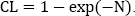
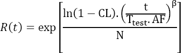
The purpose of this type of test is to demonstrate a certain level of reliability with a given confidence level. When a reliability objective must be demonstrated, the common approach is to submit the components to testing and note the number of failures. As a result, the tests may prove time-consuming and expensive and thus, in some cases, a “zero-failure” test may be used.
While such a test has the advantage of being faster and less expensive, it also has disadvantages. These are generally accelerated tests and since only one test is conducted, assumptions must be made on the acceleration law. In addition, the demonstration may fail as soon as a failure is detected. Finally, when no failure is observed, reliability cannot be estimated; however, it is possible to estimate a lower bound (for a probability of correct functioning, also known as the survival function) or a lower bound (for an MTBF). If this bound is above the objective, this means that the reliability is demonstrated.
4.2. Theoretical principle
As already noted, there are two industrial application categories for which the reliability objective is different.
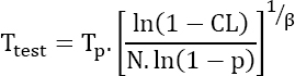
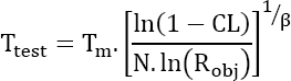
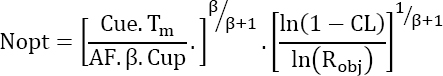
4.2.1. Non-maintained products
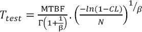
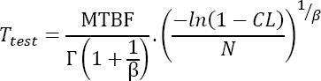
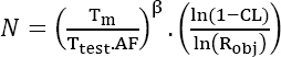
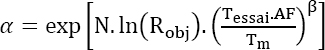
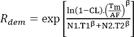
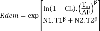
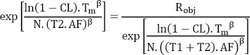
For this type of application, a Weibull distribution can be viewed as a reliability model. If Robj is the probability that the mission will be completed successfully after a duration Tm, the duration of the required test is given by:
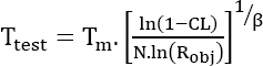
where:
- CL is the confidence level;
- N is the number of parts submitted to the test;
- β is the shape parameter of the Weibull distribution.
Demonstration
Given that a random variable X follows a Weibull distribution W(η,β) then the variable X1/β follows an exponential distribution Exp(1/η). On the other hand, the higher one-sided bound of the failure rate following an exponential distribution is given by:
Given that ![]() this yields:
this yields:
The “p-quantile” of the Weibull distribution is given by the time after which “p%” of defective parts were observed, hence:
The previous two equations lead to:
or still
or the proportion of functional parts “1- p” at the moment Tm is in fact the objective of the survival function Robj, which finally yields:
End
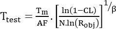
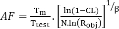
This type of test is generally conducted under accelerated conditions in order to reduce the duration of the tests, and therefore the costs. The quid pro quo is that this requires knowledge of the acceleration law that makes it possible to estimate the acceleration factor AF between the test conditions and the operational conditions. To account for the effect of physical constraints on reliability, the most commonly used model is the Acceleration Failure Time (AFT) model. This model relies on the hypothesis that an increase in the level of physical contributions accelerates the time.
Hence, equation [4.1] can be written as:
Let us interpret this last theoretical result. It can be seen that the duration of the test depends on six parameters:
- – The duration of the mission Tm, whose value is imposed by the specifications. It seems obvious that the test time is even longer as this duration is significant.
- – The probability of successfully completing the mission Robj. Similarly, this parameter is imposed by the specifications. The differentiation of Ttest with respect to Robj yields:
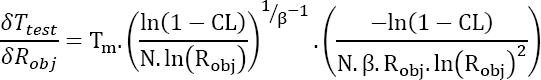
This derivative is always positive so that the test time is even longer because the probability of successfully completing the mission is high, which is a logical result.
- – The confidence level CL. This parameter is fixed before the test dimensioning.
Hence:
Here, the derivative is always positive which means the test time will be longer as the confidence level is significant. Obviously, the longer the test time, the lower the risk involved by demonstrating a reliability above the objective.
- – The parameter N, which can be controlled subject to financial considerations. It can be noted that the greater the number of parts in the tests, the shorter the testing time, but this parameter is present at a power 1/β.
- – The parameter AF, which depends on the level of physical and operational contributions of the test.
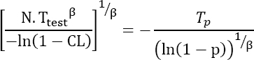
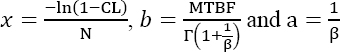
- – The parameter β. This is not known, but in the spirit of reliability demonstration, a conservative value of β is looked for. Equation [4.1] can be written as:
with
As β is by definition positive, the parameter “a” is also positive. This type of test is expected to evidence aging mechanisms, which implies β > 1. On the other hand, the confidence level CL < 1 and therefore ln(1-CL) < 0. Similarly, Robj < 1 and therefore ln(Robj) < 0. Consequently, it can be stated that x is positive. On the other hand, there are three possible cases for the value of x depending on the properties of the power function:
- – either
 and in this case it is a low value of “a” that minimizes the function f(x). Therefore, a high value of β should be chosen;
 - – or
 and in this case it is a high value of “a” that minimizes the function f(x). Therefore, a low value of β should be chosen;
 - – or x = 1 and equation [4.1] can then be written as
 irrespective of the value of β. Therefore, an arbitrary value of β can be chosen.
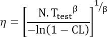
As mentioned previously, the parameters Robj, CL and Tm are fixed before the demonstration of reliability. Let us find the values of parameters N and β, for which the variable x takes values around 1.
If x > 1, a low value of β must be chosen, therefore β = 1. This leads to:
We therefore tend to consider the highest possible value of N, since the testing time is proportional to N. In fact, these two parameters (N and Ttest) can be chosen to optimize other constraints. If test duration is restrictive (either in terms of time or in terms of costs), we tend to consider the highest possible value of N in order to minimize the testing time. If, on the contrary, the tested parts are expensive, a minimum number should be considered, even if this extends the duration of the test.
If x < 1, a high value of β should be considered. However, for physical reasons, the parameter β cannot take an infinite value. Indeed, it depends on the aging mechanism that may be activated during this test. For a given component, several competing aging mechanisms are possible. It is known that the aging mechanisms depend on physical contributions applied to the tested component. This is all the more true in the case of a subset or an entire product.
As a result, when this type of test is conducted at the component level, knowing the aging mechanism that is the most likely to be activated is essential. This information is paramount for identifying the type of physical contribution to be used for the test, and therefore the acceleration law to be employed for the estimation of the acceleration factor.
When this test is conducted at the subset or product level, it is useful to know the component with the lowest reliability. All of these considerations also depend on the operational life profile. For example, if the product is watertight and the environment has low moisture content, a moist heat test is not necessary.
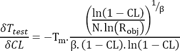
EXAMPLE.– Assume the aim is to demonstrate a reliability Robj = 92% with a confidence level CL = 80% after 10 years of operation. The reliability demonstration test is conducted under conditions such that the acceleration factor with respect to the operational conditions is AF = 100.
The first step is to observe the evolution of ![]() depending on the number of parts. In this example, Figure 4.1 is obtained.
depending on the number of parts. In this example, Figure 4.1 is obtained.
Figure 4.1. Example of demonstration of reliability of non-maintained products
It can be noted that:
- – for N∈[1 ;19], x > 1. A low value of β should therefore be chosen;
- – for N ≥ 20, x < 1. A high value of β should be chosen.
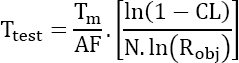
The graphical representation of the testing time as a function of N, with β as a parameter, yields Figure 4.2.
Figure 4.2. Testing time depending on the number of parts of non-maintained products
Figure 4.2 reflects the theoretical principles presented above. When the number of parts being tested is below 20, a low value of β is conservative (which yields the longest testing time). Starting with N = 20, the opposite is true. Therefore, in this example, if for other reasons (costs, testing duration, overall external dimensions of the parts being tested, etc.) we choose, for example, N = 10, a parameter β = 1 should be considered. In this specific case, the test duration is 1,691 hours.
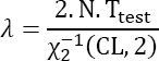
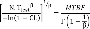
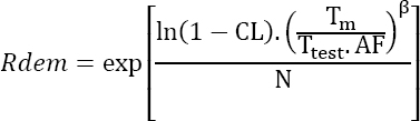
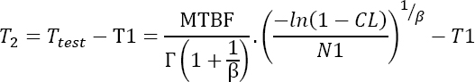
4.2.2. Maintained products
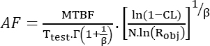
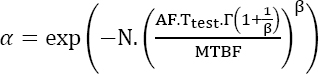
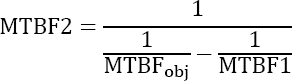
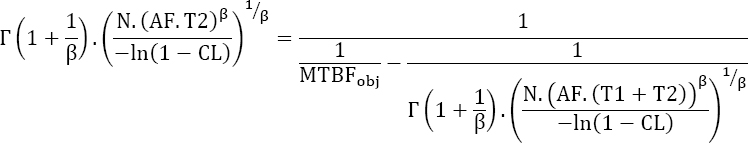
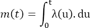
The same approach can be used to find an MTTF, instead of an observed downtime. It can then be written as:
Demonstration
As previously noted, ![]() . Furthermore, as noted in Chapter 1 of the previous book, numerically MTBF ~ MTTF. Finally, as far as the Weibull distribution is concerned, it is known that
. Furthermore, as noted in Chapter 1 of the previous book, numerically MTBF ~ MTTF. Finally, as far as the Weibull distribution is concerned, it is known that ![]() Hence, the following can be written as:
Hence, the following can be written as:
or still
End
Equation [4.3] can be written in the following form:
with
Since β is by definition positive, the parameter “a” is also positive. This type of test is expected to evidence aging mechanisms, which implies β > 1.
Then, for ![]() and hence b > 1. On the other hand, the confidence level CL < 1 and therefore –ln(1–CL) is positive. Consequently, it can be said that x is positive. On the other hand, there are three possible cases for the value of x depending on the properties of the power function:
and hence b > 1. On the other hand, the confidence level CL < 1 and therefore –ln(1–CL) is positive. Consequently, it can be said that x is positive. On the other hand, there are three possible cases for the value of x depending on the properties of the power function:
- – either x < 1, and in this case a low value of a minimizes the function f(x). Therefore, a high value of β should be chosen;
- – or x > 1 , and in this case a high value of a minimizes the function f(x). Therefore, a low value of β should be chosen;
- – or x = 1 and this yields the following condition:
 This case is numerically unlikely as N is an integer. On the other hand, equation [4.2] can be written as
  irrespective of the value of β since x = 1. An arbitrary value of β can therefore be taken.
Similar to the non-maintained products, the acceleration factor between the test and operational conditions should be taken into account. This leads to:
EXAMPLE.– Using the data from the previous example for a maintained product, there is no need for the parameter Robj. It must be replaced by an MTTF that is assumed to be MTTF = 100,000 hours.
The first step is to observe the evolution of ![]() depending on the number of parts. In this example, Figure 4.3 is obtained.
depending on the number of parts. In this example, Figure 4.3 is obtained.
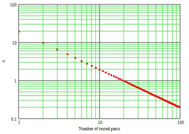
Figure 4.3. Example of reliability demonstration for maintained products
It can be noted that:
- – for N = 1, x > 1. Therefore, a low value of β should be chosen;
- – for N > 1, x < 1. Therefore, a high value of β should be chosen.
The graphical representation of the testing time as a function of N, with β as a parameter, yields Figure 4.4.
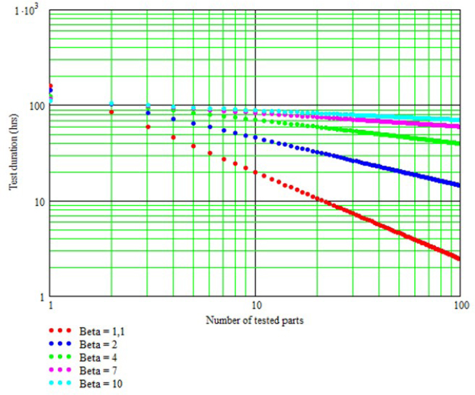
Figure 4.4. Testing time depending on the number of parts of maintained products
Therefore, in this example, if for other reasons (costs, testing time, overall external dimensions of the parts being tested, etc.) a value N = 10 is chosen, for example, then a parameter β = 10 should be considered. For this specific case, the test duration is 876 hours.
4.2.3. Estimation of parameter β
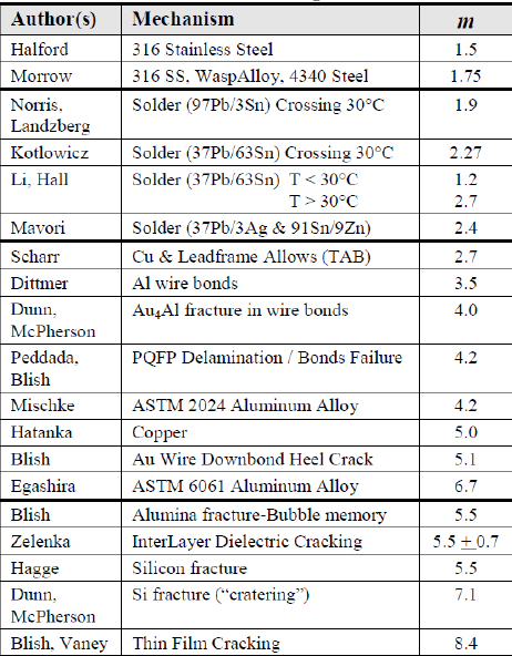
This parameter is ubiquitous in all types of tests, but its estimation is an important, albeit difficult, stage. Besides the instructions presented in the previous chapter, physical aspects can be considered. For example, for the components referred to as “mechanical”, a typical value of this parameter is in the range [1; 3] (Barringer and Barringer & Associates Inc. 2010), as illustrated in Table 4.1.
Table 4.1. Values of parameter β for mechanical components
High values of β may result when the underlying failure mechanism is mainly due to a very well-controlled physical characteristic. For example, this is the case for a broken weld of an integrated circuit on a printed circuit. It is indeed possible to have values of β exceeding 10, as illustrated in Figure 4.5.
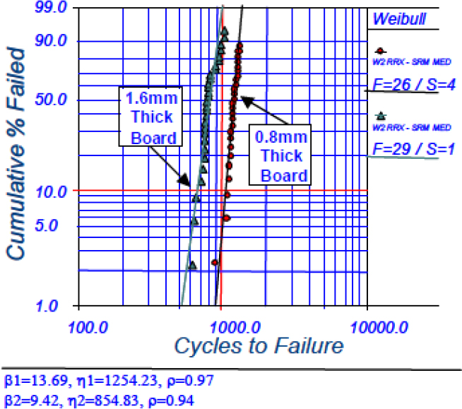
Figure 4.5. Weibull plot for the welding strength during thermal cycling
Indeed, as noted in Chapter 1 of the previous book, the parameter β was indicative of aging kinetics, which corresponds to the dispersion of time until the failure of the test components. When the failure mechanism depends on the control of geometrical dimensions and the latter are well controlled – which is the case for integrated circuits pins – the components tend to behave similarly, which involves high values of parameter β. Another example occurs when the failure results from exceeding a degradation level, for which the component being tested no longer has the expected performance. For example, this is the case for electrolytic capacitors whose capacitance decreases in time, as illustrated in Figure 4.6.
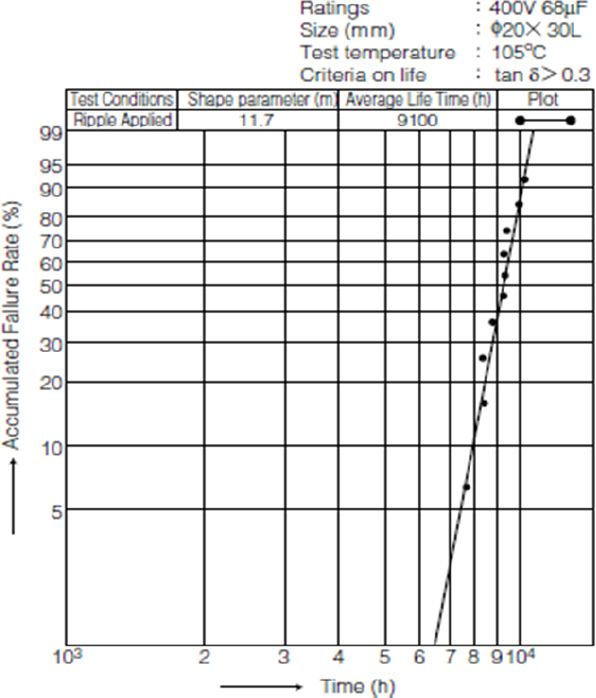
Figure 4.6. Weibull plot of electrolytic capacitors
4.2.4. Physical laws of failure
These tests are generally accelerated with respect to the operational conditions and the corresponding acceleration factor should be estimated.
Table 4.2 defines the various physical laws of failure.
NOTE.– For thermal cycling, it is also possible to use an alternative to the Coffin–Manson law. This is the Norris–Landzberg law (Landzberg 1969), defined by its acceleration factor:
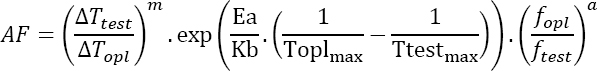
where f represents the frequency of cycles
- – The various activation energies Ea proposed in Table 4.2 are representative of various failure mechanisms. They are therefore numerically different.
Table 4.2. Physical laws of failure
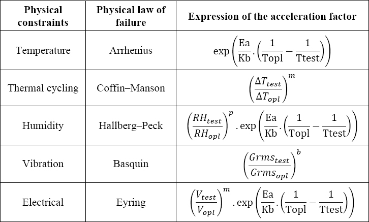
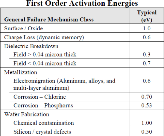
4.2.4.1. Parameter of the Arrhenius law
The Arrhenius law only has one parameter, activation energy, which depends on the failure mechanism. Various sources can be referred to for the estimation of this parameter:
- – FIDES Guide (FIDES 2009);
- – JEDEC JEP122C Standard (JEDEC 2006).
| Family of components | Activation energy |
| Integrated circuits | 0.7 eV |
| Active discrete | 0.7 eV |
| LED, photocouplers | 0.4 eV |
| Resistors | 0.15 eV |
| Fuses | 0.15 eV |
| Ceramic capacitors | 0.1 eV |
| Aluminum capacitors | 0.4 eV |
| Tantalum capacitors | 0.15 eV |
| Magnetic circuits | 0.15 eV |
| Oscillators and quartz | 0 eV |
| Relays | 0.25 eV |
| Interrupters and switches | 0.25 eV |
| Printed circuits | 0 eV |
| Connectors | 0.1 eV |
| HF and RF active components | 0.7 eV |
| HF and RF passive components | 0.15 eV |
Table 4.4 gives the activation energies used in the guide (JEDEC 2006) for semiconductors.
Table 4.4. Activation energies according to the JEDEC JEP122 standard
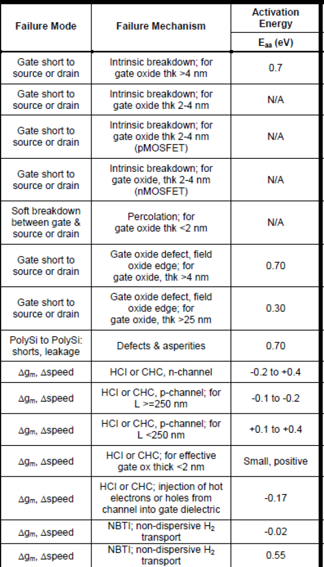
Table 4.5 gives the activation energies used in the publication (Livingston 2000) for semiconductors.
Table 4.5. Activation energy
The activation energy according to EDR (2000) for microelectronics is given in Table 4.6.
Table 4.6. Activation energy according to EDR (2000)
The activation energy according to Toshiba (2018) for TOSHIBA semiconductors is given in Table 4.7.
Table 4.7. Activation energy for TOSHIBA semiconductors
4.2.4.2. Parameters of the Coffin–Manson law
The value of various Coffin–Manson parameters is given in (Livingston 2000).
Table 4.8. Coffin–Manson coefficient according to (Livingston 2000)
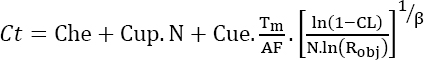
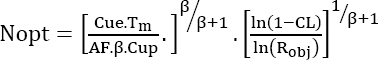
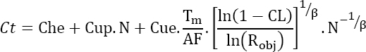
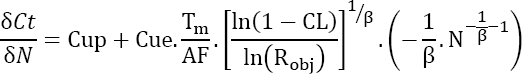
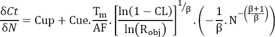
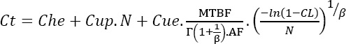
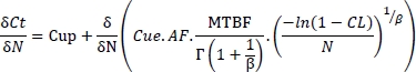
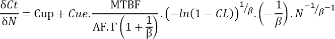
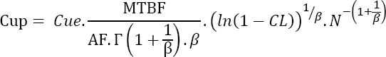
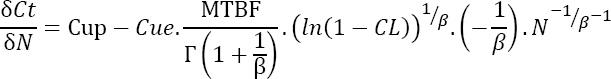
4.3. Optimization of test costs
We can also look for the number of parts that, while providing proof of reliability, also optimize the costs of such a test.
Given:
- Ct: total cost of the test;
- Cup: cost per unit for the product being tested;
- Cue: cost per hour of the test;
- Che: fixed cost of the test.
The total cost of the test is therefore:
Non-maintained products
Consequently, replacing the testing time of equation [4.2] leads to:
If it exists, the minimum cost is obtained by:
- – differentiating the total cost Ct with respect to the number of parts N being tested;
- – finding the value of N for which the derivative is zero. If applicable, this is an extremum;
- – calculating the second derivative of the total cost with respect to N. If it is positive, then a minimum is obtained.
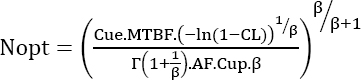
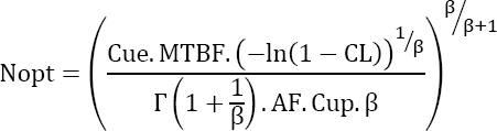
The minimum cost is then obtained by the following optimum value of N:
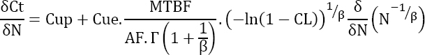
Demonstration
Equation [4.6] can be written as:
hence:
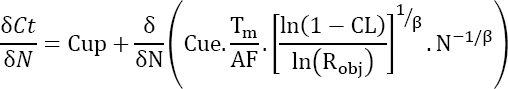
or
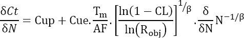
or
Consequently, there is an extremum for:
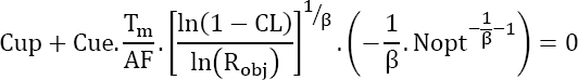
or still
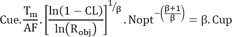
furthermore
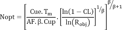
or finally
End
The extremum is a minimum since the second derivative of the total cost with respect to N is positive.
Demonstration
As previously noted:
The differentiation of this equation yields:
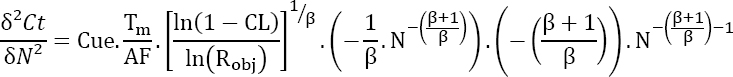
This equation is still positive, therefore Nopt is a minimum.
End
Moreover, this minimum is:

EXAMPLE.–
Che = 5,000 Cup = 1,000 Cue = 100 Tm = 10 years AF=100 CL=95% Robj = 90% β = 2
Figure 4.7 is obtained.
There is an optimum for Nopt = 38, and the total cost is 118,775.
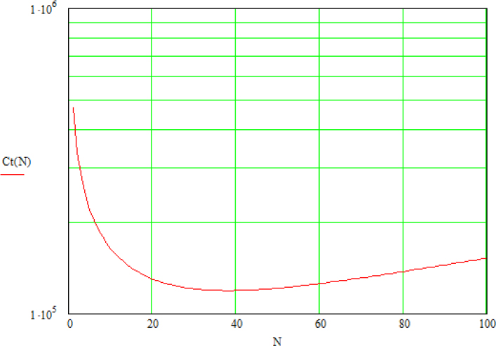
Figure 4.7. Example of optimum cost for tests of non-maintained products
Maintained products
Replacing the testing time yields:
The optimum cost, which is a minimum here, results from the differentiation of this equation with respect to the number N of parts being tested, hence:
Demonstration
or
or
Furthermore, given the search for N for which ![]()
or still
End
The extremum is a minimum since the second derivative of the total cost with respect to N is positive.
Demonstration
As previously noted:
Further differentiation of this equation yields:
This equation is still positive, therefore Nopt is a minimum.
End
Moreover, this minimum is:

EXAMPLE.–
Che = 5,000 Cup = 1,000 Cue = 100 AF=100 MTBF = 100,000 β = 2
Figure 4.8 is obtained.
Figure 4.8. Example of optimum cost of testing maintained products
There is an optimum of Nopt = 21, and the total cost is 68,618.
4.4. Specific cases
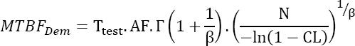
In the case of non-maintained products, when resuming equation [4.1] for the demonstration of “zero-failure” reliability, the following can be noted:
- – the probability of proper functioning or the MTBF objectives are imposed by the specification;
- – the confidence level must be fixed in advance and not adjusted depending on the intended objective;
- – the shape parameter of the Weibull law depends on the underlying failure mechanism;
- – the testing time is a variable that can be exploited, but is necessarily limited for cost and/or time problems in response to the equipment manufacturer;
- – the number of parts is a variable that can be exploited, but is necessarily limited in terms of cost and/or overall external dimensions in the test;
- – the acceleration factor is a variable that can be exploited, but is necessarily limited; the level of physical contribution of the test is limited by the manufacturer’s warranty.
This equation was arbitrarily presented in the form of a calculation of testing time with the hypothesis that the number of parts and the acceleration factor are known. Any of them could have been chosen, and this section analyzes all possible combinations.
4.4.1. Imposed number of parts
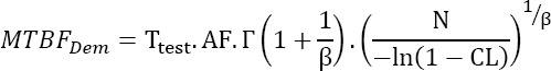
This is the case when the cost of parts is high or when there are overall external dimension problems in the testing. Therefore, the testing time must be calculated.
4.4.2. Imposed testing time
In general, the number of parts is chosen and the testing time is calculated to demonstrate the specified reliability objective. But it is possible that the testing duration is fixed, notably by the client. Therefore, the number of parts to be submitted to the test must be estimated.
Non-maintained products
In this case, equation [4.2] can be reformulated as follows:
Maintained products
In this case, equation [4.4] can be reformulated as follows:
4.4.3. Imposed testing time and number of parts
This is most often the case when the number of parts and the testing time are fixed because of high costs that are not acceptable for the project and/or the customer. In order to keep the reliability objective, the acceleration factor must be adjusted.
Non-maintained products
In this case, equation [4.2] can be reformulated as follows:
The acceleration factor depends on the physical law of failure. We recommend limiting this factor to 1,000. Indeed, the validity of the physical laws of failure is never specified and there may be a threshold below which the law is no longer applicable. Considering the example of temperature with the Arrhenius law, the FIDES methodology (FIDES 2009) indicates a validity range between –55 and +125°C (if the component is guaranteed for this range). Therefore, for an active component whose activation energy is 0.7 eV, an acceleration factor is found between the two extreme temperatures of the range [–40; +85°C], in the order of 200,000. In other terms, one hour of testing at +85°C is equivalent to ~22 years at –40°C.
On the other hand, from a physical point of view, the activation energy can be seen as a minimum energy (the kinetic energy of particles increases with temperature) that activates the chemical reaction leading to an aging mechanism. Nothing happens below this energy (hence below a certain temperature). While this is acceptable for estimating the forecast reliability (indeed, when calculating a failure rate at –40°C according to the Arrhenius law, a very low figure is found, which is numerically a good approximation of 0), it is not reasonable to use the Arrhenius law for estimating an acceleration factor under arbitrary conditions.
Maintained products
In this case, equation [4.4] can be reformulated as follows:
4.4.4. A test was already conducted and the demonstrated reliability should be estimated
Non-maintained products
In this case, equation [4.2] can be reformulated as follows:
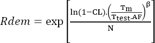
EXAMPLE.–
- Given CL = 80%;
- Tm = 10 years;
- N = 10;
- AF = 100;
- β = 3.
The demonstrated reliability is ~82.2%
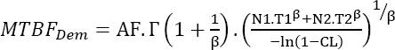
Maintained products
In this case, equation [4.4] can be reformulated as follows:
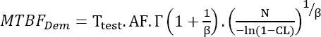
EXAMPLE.– Using the same data, the result is: MTBF_Dem ~ 134 616
4.4.5. One test was already conducted and failure to demonstrate reliability must be known
Non-maintained products
It is also possible that the test was already conducted and there is a need to assess the risk of failing the demonstration of the reliability objective. Equation [4.2] can also be written as:
By choosing a test duration of 2,000 hours, there is a 14.9% risk of failing to demonstrate the reliability objective.
Maintained products
Equation [4.4] can also be written as:
By choosing a test duration of 1,000 hours, there is a 0.2% risk of failing to demonstrate the reliability objective.
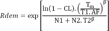
4.4.6. Two tests were conducted
4.4.6.1. Testing conditions are identical for both tests
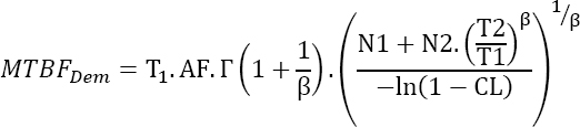
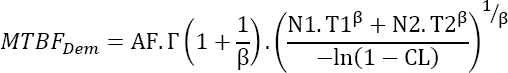
There may be two zero-failure tests under the same testing conditions (identical acceleration factors for both tests), but for a different duration and on a different number of parts. The question is: What do the two tests demonstrate?
Non-maintained products
Given
- R1: the survival probability demonstrated by test 1
- R2: the survival probability demonstrated by test 2
- N1: the number of parts in test 1
- T1: the duration of test 1
- N2: the number of parts in test 2
- T2: the duration of test 2
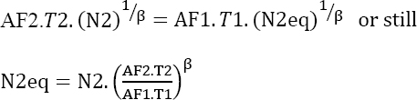
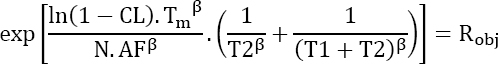
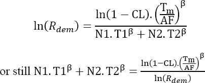
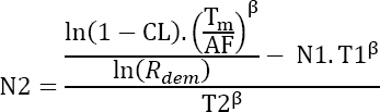
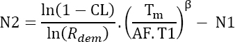
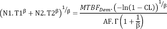
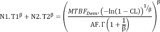
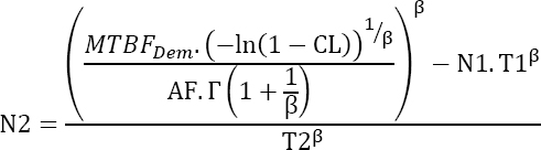
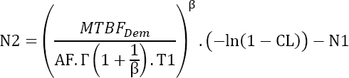
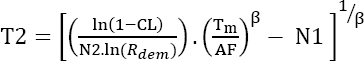
the number of parts N2eq that would demonstrate the survival probability R2 if the test duration was T1 should be found for test 2. This can be mathematically expressed as follows:
Using equation [4.15], this leads to:
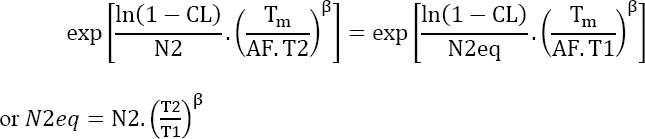
Since the two tests have the same duration, we can bring them together with the following characteristics:
- – Test duration T = T1;
- – Number of parts
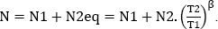
The survival probability demonstrated by the two tests is therefore:
Demonstration
As already noted, the survival function can be written as:
Consequently, under the previous conditions, the following can be written as:
or
End
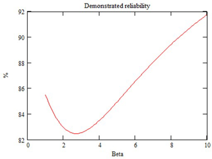
Figure 4.9. Survival function for the two tests
EXAMPLE.–
Assume the following data are available:
- – T1 = 200 hours;
- – N1 = 10;
- – T2 = 500 hours;
- – N2 = 5;
- – CL = 90%;
- – Tm = 5 years;
- – AF = 100.
The graphical representation of the evolution of this demonstrated survival function depending on β is shown in Figure 4.9.
It is easy to generalize this to “m” different tests. This yields:
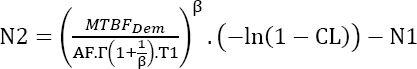
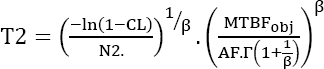
Maintained products
Given
- MTTF1, the MTTF demonstrated by test 1
- MTTF2, the MTTF demonstrated by test 2
the number of parts N2eq that would demonstrate MTTF2 if the duration of this test was T1 should be found for test 2. This can be mathematically expressed by:
Using equation [4.16], this leads to:
Since the two tests have the same duration, they can be brought together with the following characteristics:
- – Test duration T = T1;
- – Number of parts
The MTTF demonstrated by the two tests is therefore:
Demonstration
According to equation [4.17]:
Using the obtained testing conditions, the following can be written as:
or still
End
For the exponential, equation [4.22] becomes:
NOTE.– The “hours x number of components” characteristic for the exponential law is present but is often used arbitrarily.
- – Test 1 was taken as a reference, though another test could have been considered instead, without affecting the result.
EXAMPLE.– Let us take the data from the previous example, namely:
- – T1 = 200 hours;
- – N1 = 10;
- – T2 = 500 hours;
- – N2 = 5;
- – CL = 90%.
The graphical representation of the evolution of this demonstrated survival function depending on β is shown in Figure 4.10.
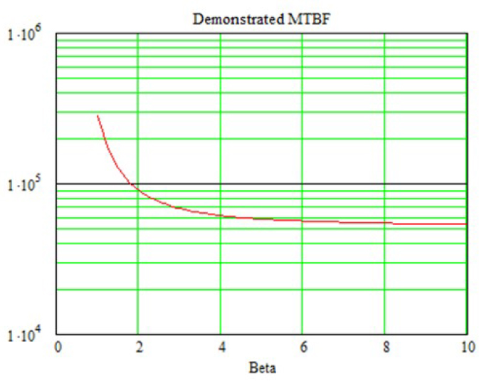
Figure 4.10. Example of MTBF demonstrated with two tests
Let us take equation [4.22] and study the limit of MTBF demonstrated when β tends to infinity. The following can be written as:
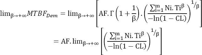
as ![]() Let us note that
Let us note that ![]() The previous equation can then be written as:
The previous equation can then be written as:
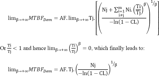
This is why an asymptote is observed in the previous figure.
4.4.6.2. Testing conditions differ for the two tests
Two zero-failure tests may be conducted for different durations and on different number of parts and, furthermore, under different testing conditions (different acceleration factors for the two tests). The question is: What do these two tests demonstrate?
Non-maintained products
The number of parts N2eq that would demonstrate the survival probability R2 if the duration of this test was T1 should be found in test 2. The following can be written as:
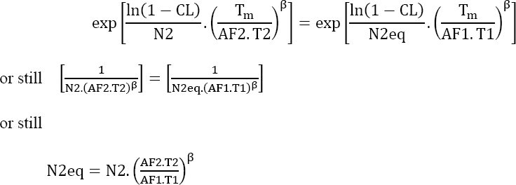
NOTE.– It can be verified that if AF1 = AF2 = AF, this leads to the equation ![]()
The demonstrated reliability is then given by:
EXAMPLE.– Let us observe the evolution of the demonstrated reliability as a function of parameter β with the acceleration factors AF1 and AF2 as parameters (N1 = 10; N2 = 5; Tm = 5 years and CL = 80%). Figure 4.11 is obtained.
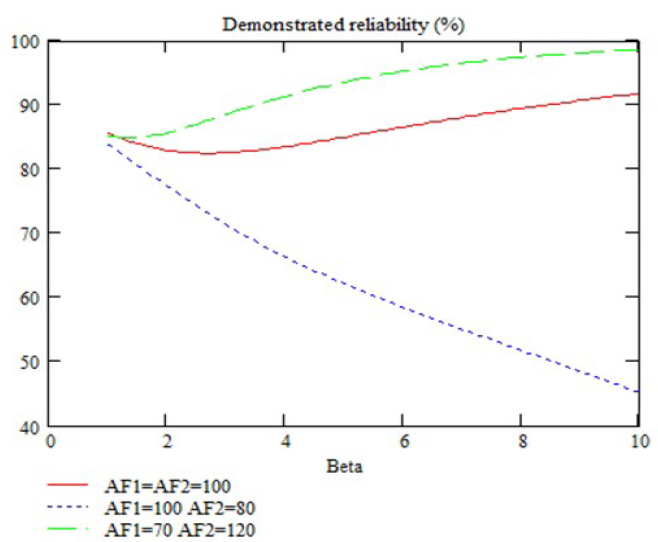
Figure 4.11. Demonstrated reliability under various conditions
This example shows that according to the value of parameters AF1 and AF2, the profile of the reliability as a function of β can be very different. Therefore, the choice of the latter parameter may prove very important.
Maintained products
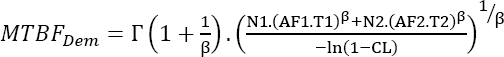
Equation [4.17] can be used to write:

or still
The demonstrated MTBF is then given by:
EXAMPLE.– Let us observe the evolution of demonstrated reliability as a function of parameter β with acceleration factors AF1 and AF2 as parameters (N1 = 10; N2 = 5; Tm = 5 years and CL = 80%). Figure 4.12 is obtained.
Here, the parameter β has little influence, notably for β > 2.
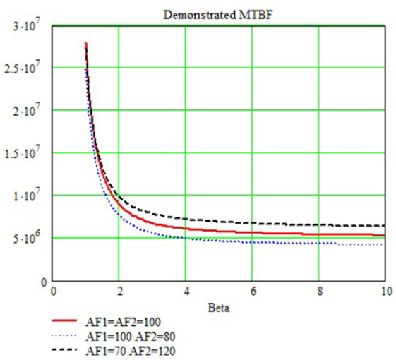
Figure 4.12. Reliability demonstrated under various conditions
4.4.7. A second test is conducted
The following situation may be encountered: a test referred to as a “reliability test” was reported to have been conducted under certain conditions. Since no failure was observed, the question was if the test was relevant in terms of reliability. Since this type of test is generally not dimensioned to demonstrate any level of reliability, the result was irrevocable: the estimated reliability level does not meet the demand.
It may be said that a miracle was needed for this to happen. Indeed, in order to estimate the reliability level demonstrated by this test, the “zero-failure reliability demonstration” theory was used, under certain hypotheses.
The project members then asked the following question: What further test should be conducted to demonstrate the reliability demand?
Several cases can be expected:
- – A dimensioned test that meets the reliability demand is conducted. While it may prove profitable in terms of reliability, it is not in terms of cost as the first test was useless, nor is it profitable in terms of time. It was consequently rejected.
- – Taking into account the first test conducted makes it possible for a second test to be dimensioned, on different parts, meeting the reliability demand.
- – A third option was proposed, namely to continue the test on the parts that were subjected to the first test. Three situations are then to be expected.
4.4.7.1. Testing conditions similar to the first test are maintained
The testing time Ttest, which should have been taken into account to demonstrate the reliability demand, is calculated. It is then sufficient to calculate the duration of the second test as a function of the duration of the first test:
EXAMPLE.–
Non-maintained products
A first test was conducted with the following conditions:
- – CL = 80%;
- – T1 = 200 hours;
- – AF = 100;
- – N1 = 10;
- – Robj = 92%;
- – β = 2.
If N2 = N1, this yields: 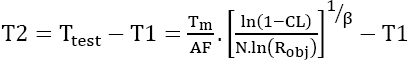
The result is T2 = 1,132 hours
Maintained products
A first test was conducted under the following conditions:
- – CL = 80%;
- – T1 = 200 hours;
- – AF = 100;
- – N1 = 10;
- – MTBF = 1000 hrs;
- – β = 7.
The result is T2 = 623 hours
4.4.7.2. Similar conditions to the first test, with additional new parts
The same testing conditions as for the first test are maintained. For time problems, the duration of the second test is fixed and other (new) parts are added to meet the reliability objective. The situation can be synthesized as follows:
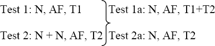
Non-maintained product
As the two tests are independent, the following can be written as:
Or still
Or, furthermore: ![]() hence:
hence:
or more simply
This equation has no analytical solution and should therefore be solved numerically.
Non-maintained product
It can be written that: ![]()
In our case, this yields:
It is known that: ![]()
This equation must be solved, with T2 being the unknown. Since it has no analytical solution, it must be solved numerically.
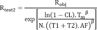
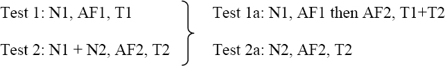
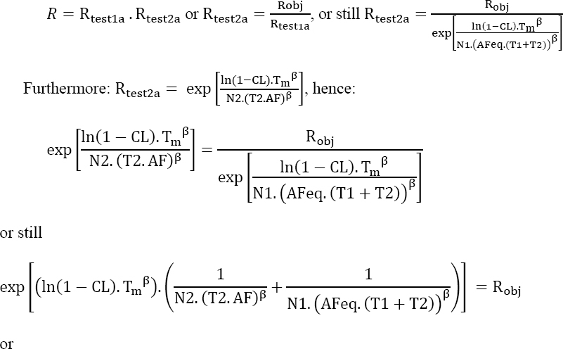
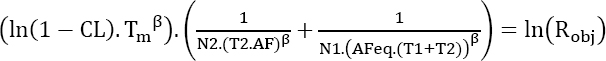
4.4.7.3. The conditions of the first test are changed, the parts are the same
The testing conditions of the first test are changed, as they require additional time, which is too significant for the project. This is schematically represented in Figure 4.13.
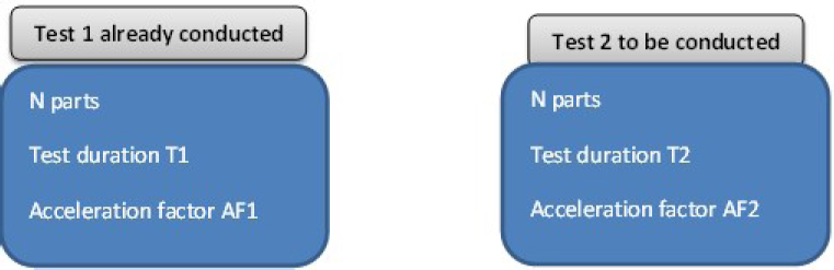
Figure 4.13. Principle of testing the same parts under different conditions
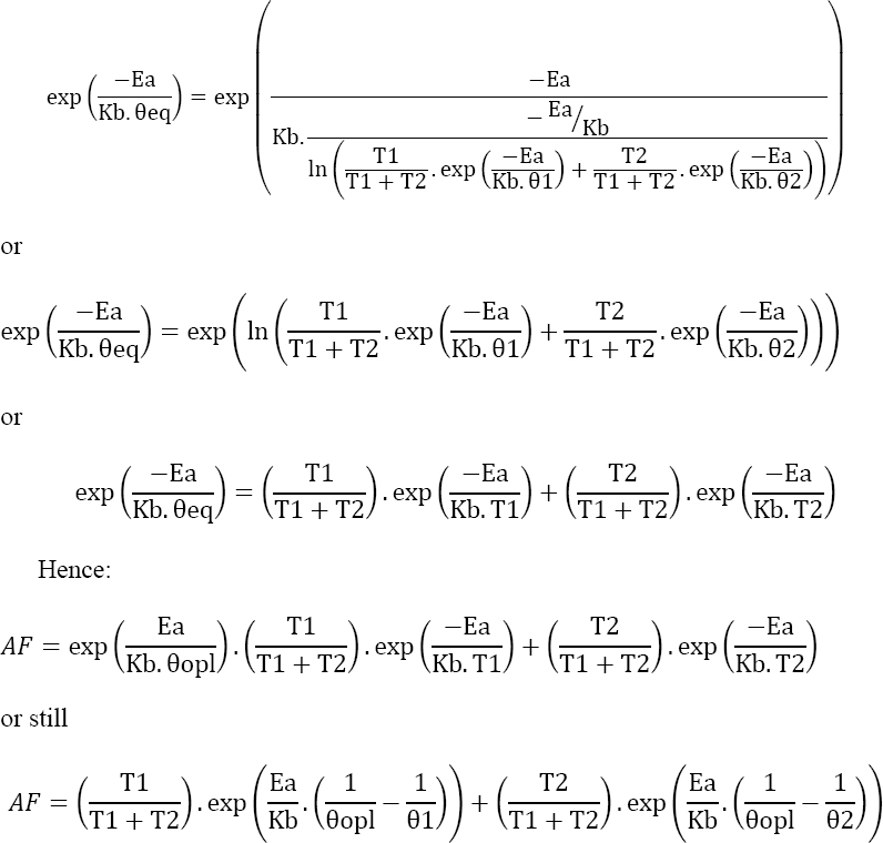
To illustrate our point, let us consider the case of temperature, which is often the physical contribution of interest. The tested parts are therefore subjected to the following temperature:
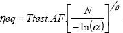
The Sedyakin principle (Sedyakin 1966) is used to estimate a temperature that is equivalent in terms of reliability to the temperature profile given in Figure 4.14. It can then be shown that, in this case (Bayle 2019):
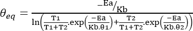
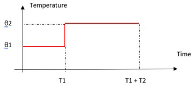
Figure 4.14. Temperature profile under different conditions
Hence, the acceleration factor of this test, with respect to the operational conditions, is given by:
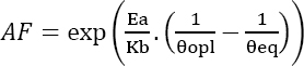
Therefore, the acceleration factor is given by:

Demonstration
From the Arrhenius law, we can write:
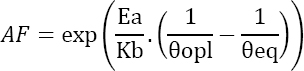
Or still
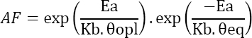
Equation [4.28] can be used to write:
End
This can be generalized to “n” consecutive levels of temperature of duration Ti and of values θi:
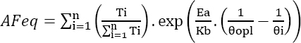
This leads to a single test with the following characteristics:
- – N parts under test;
- – test duration T1+T2;
- – acceleration factor AFeq according to equation [4.31].
4.4.7.4. The conditions of the first test are changed with the same parts and new parts are added
While the first test was conducted with a fairly low acceleration factor, it is possible that with the same acceleration factor, this could lead to a second test of long duration or involving a significant number of parts that are incompatible with the constraints of the project and/or those of the system manufacturer. The proposal is therefore to modify the testing conditions in order to increase the acceleration factor (AF2 > AF1).
This situation can be synthesized as follows:
Non-maintained products
As the two tests are independent, the following can be written as:
This equation must be solved, with AF2 being unknown. This has no analytical solution; therefore, it must be solved numerically.
4.4.7.5. The same testing conditions are maintained for the second test
This amounts to stating that the testing conditions are not similar to those of the first test, meaning that the acceleration factor is the same.
First case: the duration of the test is the same, but the quantity of tested parts is adjusted to maintain the reliability objective, which is T1 = T2. Therefore, the question is: How many parts are needed for the second test?
Non-maintained products
The result is:
Demonstration
According to equation [4.16]: 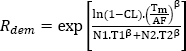
The logarithm of both members of the equation yields:
or still
Or finally, since T1 = T2
End
Maintained products
The result is:
Demonstration
According to equation [4.17]: ![]()
This leads to:
or still
or still
Or finally, since T1 = T2
End
Second case: The same quantity of parts is tested, but the test duration is adjusted to meet the reliability objective. Therefore, the question is: How much time T2 should the second test take?
Non-maintained products
Using the same procedure as before, we obtain:
Maintained products
Similarly, we have:
4.4.8. Reliability objective is a failure rate
Certain customers specify a failure rate objective λobj upon mission completion Tm, which here is:
Demonstration
Using the expression of the survival function in equation [4.16], we get:
The differentiation of this equation with respect to t yields:

Consequently, the failure rate is given by:
Hence
Or finally
End
NOTE.–
- – This leads to the formulation of the Weibull distribution with
- – For the exponential law (β = 1), we get:
This leads to the MTTF formula.
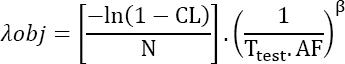
- – Depending on the values of parameters, this failure rate has a maximum of
 as shown in Figure 4.15
Figure 4.15. Objective failure rate
It is this value of β that will be taken into account for the dimensioning of the corresponding test
- – This is only applicable to non-maintained products. For maintained products, the failure rate has no meaning; therefore, the notion to be used is Rocof. For the sake of simplicity, while remaining conservative for the demonstration of reliability, the asymptotic value of Rocof given by (Bayle 2019) is employed:
We therefore come back to the previously studied cases for MTBF.
4.4.9. Reliability data are available from the manufacturer
At the component level, particularly for active components such as integrated circuits, the manufacturer may have conducted reliability tests that are generally referred to as “reliability reports”. In this case, prior to launching a reliability test, it may be wise to use this data. Generally, the reliability estimations are “0 failure” data, so the proposed theory naturally fits.
If no reliability data are available from the manufacturer, the component may meet a given standard.
4.4.9.1. Manufacturer data
Consider the example of an integrated circuit for a testing temperature HTOL (XILINX 2020).
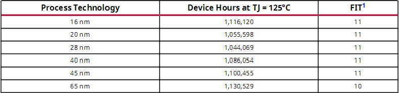
The failure rate is calculated from the following equation:
Considering the 16 nm technology, for example, the mentioned failure rate is 11 Fits at 55°C for a confidence level of 60% and an activation energy of 0.7 eV.
Non-maintained products
Assume the following data are given:
- – Robj = 98%;
- – Tm = 10 years;
- – Topl = 40°C;
- – CL = 80%.
The proper functioning probability is given by: ![]() At the time
At the time ![]() Let us now calculate the acceleration factor between the operational conditions and the manufacturer. This yields:
Let us now calculate the acceleration factor between the operational conditions and the manufacturer. This yields:
On the other hand, the specified confidence level differs from the one used by the manufacturer. Therefore, the manufacturer failure rate must be recalculated with this confidence level, which yields λ = 18.5 Fits.
Therefore, the resulting reliability is:
The 98% objective is then met.
Maintained products
Here, the objective is MTBF = 10,000,000 hrs. Using the same operational conditions as before, we get: ![]() The objective is therefore met.
The objective is therefore met.
4.4.9.2. Standard data
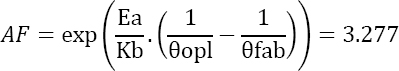
Consider the example of a quartz resonator for the case of temperature. No reliability data are available for the component, but in certain industrial fields, there are standards that qualify the components. This is notably the case for the automotive standard (Automotive Electronics Council 2010) for passive components.
Table 4.9 summarizes the tests conducted.
Table 4.9. Tests conducted on a quartz crystal according to the Automotive Electronic Council (2010)
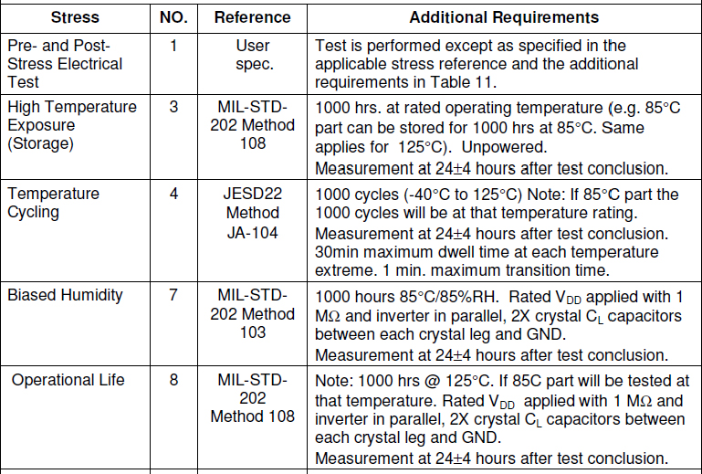
Resuming the case of temperature (operating life), the characteristics of the test conducted are as follows:
- – Ta = 125°C;
- – Duration 1,000 hrs;
- – Batch size: N = 77 parts.
A 0.55 eV activation energy is considered.
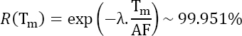
Non-maintained products
Assume the following data are available:
- – β = 2.1;
- – Tm = 10 years;
- – Topl = 40°C;
- – CL = 80%.
The reliability demonstrated by these tests is obtained from equation [4.15]:
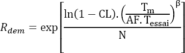
A reliability of ~97.4% is thus demonstrated.
Maintained products
The reliability demonstrated by these tests is given by equation [4.16]:
An MTBF of 435,103 is thus demonstrated.
4.4.10. Demonstration of reliability at the product level
The method proposed for the various cases previously studied applies to non-maintained products, which is rather applicable at the component or even subset level.
As for tests at the product level, these are potentially repairable. The classical hypothesis at the “product” level is that of minimal maintenance, meaning that repairing defective component(s) restores the product reliability state before failure. This repair process can be modeled by a non-homogeneous Poisson process (NHPP). For this type of process, the average number of failures as a function of time follows a Poisson law of parameter m, given by:
where λ is the failure rate of the NHPP process.
The relation that can be used to obtain the necessary test duration Ttest is given by:
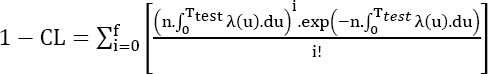
where:
- n is the number of products being tested;
- f is the number of breakdowns observed;
- CL is the confidence level.
When the product is mature, this model is completely applicable. The average number of failures is then:
Generally, a product is referred to as mature if it can be modeled by a homogeneous Poisson process (HPP). In this case, formula [4.37] can be written as:
If there is no failure, f = 0 and the above becomes:
or still
4.4.11. Taking into account a complex life profile
The previous sections featured a level of physical contribution limited to a single value, but reality is far more complex. Therefore, this chapter proposes a methodology that brings a complex level of physical contribution (life profile) to a single value.
This is approached from the perspective of temperature as this raises most of the problems. First, it is important to give several explanations on the construction of a life profile. Logically, the system manufacturer should provide a life profile as a specification. Based on this data, the equipment manufacturer breaks down the life profile, taking into account characteristics that are intrinsic to its product (temperature increase, thermal time constant, damping, etc.).
A life profile is generally periodic, in the sense that it is re-enacted a certain number of times throughout the time that a product is operational. Hence, the life profile is often deployed over a calendar year. The levels of physical contributions are generally not constant due to product activity, which varies with time. The fact that physical laws of failure are only valid for constant levels of physical contribution requires the decomposition into various stages for which this hypothesis is valid. Very often, these stages correspond to operational activities of the product. For further details on the notion of life profile, refer to the FIDES guide (FIDES 2009).
4.4.11.1. The thermal time constant is small compared to the stage duration
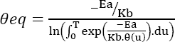
In this case, the temperature can be considered constant for each stage. Given a life profile composed of “p” distinct stages of duration Ti and temperature θi, and using the Sedyakin principle (Sedyakin 1966; Bayle 2019), an equivalent temperature can be found:
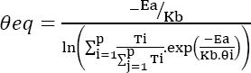
The acceleration factor AF can then be easily deduced.
EXAMPLE.– Consider the following life profile:
Given p = 5, Ea = 0.7 eV, then: θeq ~ 58.4°C
4.4.11.2. Thermal time constant is not negligible
The previous formula cannot be used because temperature is not constant over the considered stage. In this case, we have (Bayle 2019):
This equation has no analytical solution; therefore, it must be solved numerically.
NOTE.– The product can generally be considered a first-order product so that the temperature evolution follows exponential branches.