
5
Reliability Management
5.1. Context
In order to produce a mature product, equipment manufacturers try their best to reach a reliability level that is higher than the one specified, and most of all, that is constant throughout its operation duration. Three situations can be encountered:
- – the ideal case is when the product is mature;
- – the case when reliability increases is often encountered in the industry. This type of phenomenon is clearly preferable, since improving reliability involves very significant costs. This phenomenon is very often due to design flaws, which, by their nature, affect the whole range of operational products, and have a strong impact on reliability, youth failures, etc.;
- – reliability degradation is observed over time. This is generally due to the premature aging of components.
It is therefore essential to make all of the efforts necessary to avoid youth and aging failures. Youth failures can only be filtered out by specific (burn-in, run-in) tests conducted before delivery to the equipment manufacturer. As for aging failures, specific analyses or last resort tests can be proposed.
For a maximum reduction of the probability of these two dreaded scenarios, the following methodology is proposed, as illustrated in Figure 5.1. Each of the stages proposed in Figure 5.1 is defined in the following sections.

Figure 5.1. Overview diagram of product reliability management
5.2. Physical architecture division
This stage involves the division of the product into various subsets based on the failure physics and architecture of the product for which reliability estimation is possible. This analysis generally leads to several levels, ranging from the highest, the product itself, to the lowest, a failure mechanism of a component (see Figure 5.2).
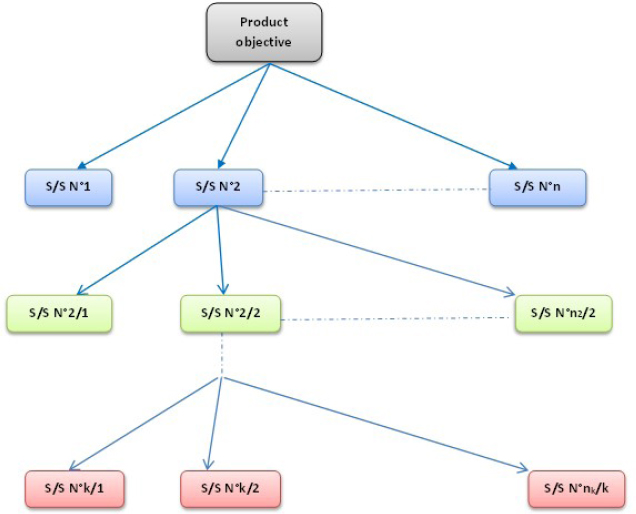
Figure 5.2. Principle of product division into subsets (S/S)
5.3. Classification of subsets
Among these various estimation methods, some are referred to as “classical”, in the sense that this estimation relies on the existing data (e.g. bill of materials + predicted reliability models), and the others are considered to be specific.
5.4. Allocation of initial reliability
The allocation of the initial reliability involves the equidistribution of the reliability objective to each of the previously defined subsets. It takes two different forms, according to the type of maintenance undergone by the product.
Non-maintained products
The initial reliability is allocated using the objective survival function according to the following relation:
where n is the number of subsets.
Based on the estimations of reliability of the subsets referred to as “1st level”, the reliability objectives of the subsets referred to as “low level” can be reallocated.
Maintained products
The initial reliability is allocated using the following relation:
According to these principles, all of the subsets of the product have an allocated reliability.
5.5. Estimation of the reliability of subsets
Each operational subset must be classified according to Table 5.1.
Table 5.1. Classification of subsets
| Estimation type | Estimation method |
| Predicted reliability | FIDES/NPRD 2017 |
| Feedback | PLP power process |
| Manufacturer data | Reliability report |
| Zero-failure demonstration | Weibull – GLL model |
| Reliability tests | Weibull – GLL model |
Some methods for building product maturity have already been described. One of the conditions is having a realistic predicted reliability method. The term realistic means that it should be of the order of magnitude of the product reliability observed during its operation. The FIDES methodology was therefore chosen as it seemed to be the most appropriate.
Chapter 6 presents some other methods for the confirmation of product maturity. One of them involves the estimation of the observed product reliability.
It is therefore essential to make sure that these two estimations are homogeneous, meaning that there is no significant difference between them. This task is not as simple as it seems. Indeed, it is not sufficient to calculate the ratio between the predicted and operational failure rates in order to answer this question (Giraudeau 2017). What are the values of this ratio starting with which a difference may be judged as significant?
To propose a more rigorous method, the following example is considered.
Assume that coins are being manufactured. One of the requirements is that these coins are balanced, meaning that the probability of having heads or tails must be equal to 50%. This is impossible in practice and an uncertainty should be considered on this value, which is purely theoretical. Assume that an uncertainty of 0.1% is deemed satisfactory.
In order to verify this, a test must be conducted on a sample of coins that are representative of those being subsequently introduced. A coin is tossed several times, and the result is illustrated as follows.

We can note that the number of heads and tails is not 50% each, as the results show 56% tails. Should we conclude that the coin is not well balanced?
To attempt to answer this, let us toss a coin several times once again. The results are illustrated in Figure 5.3.

Figure 5.3. Example of how the proper manufacturing of coins can be verified
The following can be noted:
- – the tails probability is never or very rarely 50%;
- – the sequence of tails and heads is never the same from one coin to another;
- – the probability of having tails when considering all of the data is close to 50%.
Indeed, it is clear that a hypothesis must be formulated and tested with respect to the available data. For this example, the hypothesis (referred to as a null hypothesis) is:
“The coin is well balanced”.
Two errors are therefore possible:
- – first, to consider that the coin is well balanced, when, in fact, it is not;
- – second, to consider that the coin is not well balanced, when, in fact, it is.
Obviously, it would be ideal to find a process that minimizes both risks of error at the same time. Unfortunately, it can be shown that they are inversely correlated, meaning that any process that reduces the first error generally increases the second and vice versa. A choice between the two errors will therefore have to be made, so that the error to be avoided is the more significant one.
This is a difficult choice, as it generally depends on several parameters. The risk of the first error can be legitimately minimized to avoid the introduction of coins that do not comply with specifications. However, from an economical perspective, it is possible to consider that the second error should be minimized.
Moreover, it is also important to consider the rightful rejection of the hypothesis that the coin is well balanced. This is referred to as the power of the test. There are two reasons why this notion is important:
- – the power of the test can be used to choose between tests by considering the one with the highest power;
- – it is strongly recommended to consider a power of at least 50% in order to decide on the result of the tests conducted.
To resume the case of interest here, it is therefore preferable to minimize the statement that predicted reliability is consistent with the experience feedback when this is not the case. On the other hand, we must make sure that the power of the test is equal to or greater than 50%.
The proposed method involves the execution of the following stages, given in the sections below.
5.5.1. Consistency with the experience feedback
It is important to make sure that the predicted reliability is within the range of confidence of the observed reliability.
- – A risk level is fixed in advance, generally of 10%.
- – It should be recalled that predicted reliability makes the hypothesis that the observed failures follow an exponential law of parameter λp. Therefore, for the comparison to make sense, the experience feedback data should follow a homogeneous Poisson process of parameter λ.
- – Given N the number of breakdowns observed and T the total time of observation, λ is estimated by

- – The bounds of the confidence interval (at the level 1 – α) of λ are calculated with the following relations (Rigdon and Basu 2000):

If ![]() then the predicted reliability is statistically consistent with the data.
then the predicted reliability is statistically consistent with the data.
If ![]() then the predicted reliability is not statistically consistent with the data.
then the predicted reliability is not statistically consistent with the data.
5.5.2. Estimation of the power of the test
The power of this test is the following: ![]() which is a probability that depends on the actual value of Lambda, which is unknown. The objective is then to calculate, depending on the actual value of λ, the value
which is a probability that depends on the actual value of Lambda, which is unknown. The objective is then to calculate, depending on the actual value of λ, the value ![]()
![]()
This calculation is very likely mathematically impossible, but a simulation-based numerical approach can yield this curve (or function). The following algorithm is proposed.
5.5.3. Simulation algorithm
The parameters λp, N and T are known. Here, T is fixed and N is the realization of a Poisson random variable of parameter λ x T. For each value of a set of values of λ (around λp, but different from λp), a large number of random variables is simulated following a Poisson distribution of parameter λ x T and the percentage of ![]() is calculated.
is calculated.
This percentage is an estimation of the power of the test. It is known that if λ tends to λp, then this percentage tends to (α = 1 – NC). It is also known that when λ is farther from λp, this percentage tends to 1. This curve can be used to decide, for an a priori fixed power, the possible gap between λ and λp through the test accepted λp. We then obtain:

EXAMPLE 5.1.– Consider the following data:
| – Predicted failure rate | λp = 2.2.10-3; |
| – Acceptable tolerance | Tol = 30%; |
| – Risk level | α = 10% |
| – Cumulative observation time | T = 4,000 hours; |
| – Number of observed failures | Nb_Failures = 8; |
| – Number of simulations | Nb_Simulation = 1,000. |
Therefore, the predicted failure rate interval is:
which is then:
The credibility curve in Figure 5.4 is obtained.

Figure 5.4. Credibility curve example 5.1
The credibility interval of the predicted failure rate is:
Since the credibility interval is larger than the tolerated uncertainty interval, no conclusion can be drawn when given the validity of a predicted failure rate ![]() the observation time T must be increased!
the observation time T must be increased!
EXAMPLE 5.2.– Consider the following data:
| – Predicted failure rate | λp = 2.2.10-3; |
| – Acceptable tolerance | Tol = 30%; |
| – Risk level | α = 10% |
| – Cumulative observation time | T = 10,000 hours; |
| – Number of failures observed | Nb_Failures = 10; |
| – Number of simulations | Nb_Simulation = 1,000. |
Therefore, the predicted failure rate interval is:
which is then:
The credibility curve in Figure 5.5 is obtained.

Figure 5.5. Credibility curve example 5.2
The credibility interval of the predicted failure rate is:
This is a similar conclusion to the previous one, though the credibility interval is smaller.
EXAMPLE 5.3.– Consider the following data:
| – Predicted failure rate | λp = 2,2.10-3; |
| – Acceptable tolerance | Tol = 30%; |
| – Risk level | α = 10% |
| – Cumulative observation time | T = 50,000 hours; |
| – Number of observed failures | Nb_Failures = 100; |
| – Number of simulations | Nb_Simulation = 1,000. |
Therefore the predicted failure rate interval is:
which is then:
The credibility curve in Figure 5.6 is obtained.

Figure 5.6. Credibility curve example 5.3
The credibility interval of the predicted failure rate is:
With the credibility interval smaller than the tolerated uncertainty interval, a conclusion can be drawn referring to the validity of the predicted failure rate with respect to REX.
5.6. Optimal allocation of the reliability of subsets
For certain subsets, it was therefore possible to have a reliability estimation from the predicted reliability, experience feedback or data provided by the manufacturers of components. However, this reliability estimation was not possible for others, as a test was needed for this purpose (reliability demonstration, reliability test).
The optimal allocation of reliability therefore involves setting the reliability of subsets for which an estimation was possible, and depends on this data reallocating the reliability objectives to subsets that could not have such an estimation. These new objectives allow one of the following:
- – to dimension the reliability demonstration test;
- – to verify, based on the reliability model built by the reliability test, whether the objective is met or not. If the objective is not met, a new reallocation of reliability can be made to meet the reliability objective at the product level.
5.7. Illustration
Assume that the architecture of the studied product is illustrated in Figure 5.7.
Reliability allocation for non-maintained products
Assume that the reliability objective is Robj = 92% at the time Tm = 10,000 hours. Since there are three subsets (DC/DC converter, fan and speed measurement), the reliability objective for the subsets of the first level is:
For the fan, given that there are no lower-level subsets, the following relation can be written:

Figure 5.7. Illustration of reliability management
For the subsets of the second level, the reliability objective is given by:
For the energy reserve, the booster and the digital electronics, given that there are no subsets of lower level, the following can be written:

For the level 3 subsets, the reliability objective is given by:
It can be written that:

A diagram is obtained (see Figure 5.8).

Figure 5.8. Initial reliability allocation of the subsets in case of reliability objective
Reliability allocation for maintained products
Assume that the reliability objective is MTBFobj = 10,000 hours. The reliability objective for the level 1 subsets is, considering there are three subsets (DC/DC converter, fan and speed measurement):
For the fan, since there are no low-level subsets, it can be written that:
For the level 2 subsets, the reliability objective is given by:
For the energy reserve, booster and digital electronics, since there are no low-level subsets, it can be written that:
It can be written:

A diagram is obtained (see Figure 5.9).

Figure 5.9. Initial reliability allocation of the subsets in case of MTBF objective
The reliability of the previously defined subsets should now be defined. The estimations in Table 5.2 are proposed.
Table 5.2. Reliability estimation methods for the subsets
| Estimation type | Estimation method |
| Fan | Manufacturer data |
| Energy reserve | FIDES |
| Booster | FIDES |
| Digital electronics | FIDES |
| Speed sensor | Reliability demonstration |
| Voltage reference | Accelerated test |
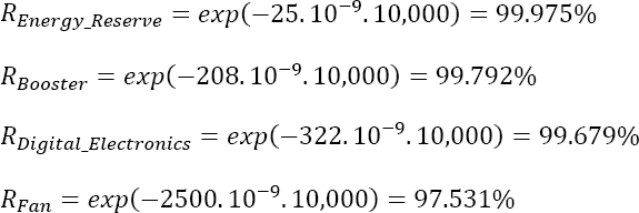
For the estimations made with FIDES, the results are:
- – λ_Energy_Reserve = 25 Fits;
- – λ_Booster = 208 Fits;
- – λ_Digital_Electronics = 322 Fits.
For the fan, the manufacturer guarantees a failure rate of:
- – λ_Fan = 2,500 Fits.
Non-maintained products
With the estimated failure rates being constant, the reliability can be estimated by the relation:
This yields:
Given this data, the other subsets can be reallocated. The following can be written:
Hence:

Consequently, the reliability of the Speed_Sensor and voltage reference subset can be estimated as follows:

A new diagram is obtained (see Figure 5.10).

Figure 5.10. Reliability allocation of the subsets in case of reliability objective after reliability prediction
The objective of reliability demonstration for the speed sensor is therefore 97.393%. For the voltage reference, it must be shown that the reliability model obtained by accelerated tests also leads to a reliability of 97.393%.
Maintained products
With the estimated failure rates being constant, the reliability can be estimated by the relation:

This yields:

Given this data, the other subsets can be reallocated. The following can be written as:
Hence:

Consequently, the reliability of the Speed_Sensor and voltage reference subset can be estimated as follows:

A new diagram is obtained (see Figure 5.11).

Figure 5.11. Reliability allocation of the subsets in case of MTBF objective after reliability prediction
The reliability demonstration objective for the speed sensor is therefore 20,630. For the voltage reference, it should be shown that the reliability model obtained by accelerated tests also leads to an MTBF objective of 20,630.
Reliability demonstration for the speed sensor
Assume that the speed sensor is temperature sensitive and its activation energy is given by Ea = 0.45 eV. On the other hand, the life profile of the product over a one year period is given in Table 5.3.
Table 5.3. Parameters of mission profile example
| Description of the stage | Stage duration (hrs) | Stage temperature (°C) |
| Non-operation | 2,760 | 15 |
| Operation | 6,000 | 45 |
Based on Sedyakin’s principle (Sedyakin 1966; Bayle 2019), an equivalent temperature of 39.3°C can be found (exp(Ea/Kb.(1/Teq – 1/Ttest) = exp(0.45/8.617e-5.(1/(273 + 39.3) – 1/(273 + 105))) # 18.3).
Assume that the test data are fixed by:
- – the number of speed sensors under test = 10;
- – the test temperature = 105°C.
Consequently, the acceleration factor of the test is: AF # 18.3.
Non-maintained products
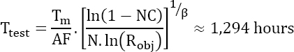
Knowing that the objective to be demonstrated is ![]() the required test time is:
the required test time is:
Maintained products
Knowing that the objective to be demonstrated is ![]() the required test time is:
the required test time is:

Reliability test for the voltage reference
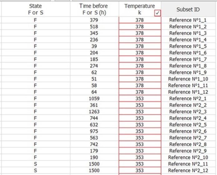
Assume that the voltage reference is temperature sensitive. Our proposal is to conduct two tests on 12 parts under the following conditions:
- – Test 1 Tj = 105°C;
- – Test 2 Tj = 80°C;
- – Maximal duration of each test = 1,500 hours.
The data in Table 5.4 was obtained.
Table 5.4. Results of the accelerated tests of reliability
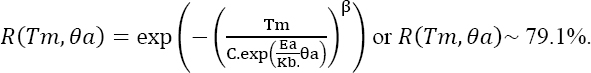
Given the temperature sensitivity, a Weibull–Arrhenius model is chosen, whose survival function is given by:

The parameters of the model to be estimated are therefore:
- – parameter β;
- – activation energy Ea;
- – scale factor C.
The maximum plausibility method yields:
- – β_Estimated ~ 1.43;
- – Ea_Estimated ~ 0.68;
- – C_Estimated ~ 2.08 10-7.
Figure 5.12 presents the Weibull paper plot.

Figure 5.12. Weibull plot voltage reference reliability test
Figure 5.13 represents the same plot, but depends on time and temperature.
Non-maintained products
Based on the data of the accelerated test, the survival function of the voltage reference under operational conditions can be estimated:
Consequently, the survival function at the analog electronics level is given by:
The survival function at the level of speed measurement is given by:

Figure 5.13. 3D Weibull plot voltage reference reliability test
The survival function at the product level is given by:
or
The objective of 97.393% is not met at the level of voltage reference and therefore at the product level.
A diagram is obtained (Figure 5.14).

Figure 5.14. Final reliability allocation of the subsets in case of reliability objective
Maintained products
Using the data of the accelerated test, the survival function of the voltage reference under operational conditions can be estimated as follows:
The objective of 20,630 is met.
The MTBF at the product level can be estimated based on various estimated MTBF. For the analog electronics, the MTBF is given by:

For the speed measurement:

Therefore, at the product level:
or
Finally, a new diagram is obtained (see Figure 5.15).

Figure 5.15. Final reliability allocation of the subsets in case of MTBF objective
5.8. Definition of design rules
For certain components whose technology evolves rapidly, it is reasonable to consider the possibility of observing failure mechanisms, all the more so as the life profile duration tends to increase in most of the industrial applications. This is particularly the case for complex digital components (microprocessor, flash memories, FPGA, etc.) with the well-known Moore’s law (Moore 1965). In order to avoid any aging problems, a manufacturer may decide to make electronics designers adhere to strict design rules. As an illustration, let us consider the virtual example of a digital component subjected to the following aging mechanisms:
- – Hot Carrier Injection (HCI);
- – Thermal Dependent Dielectric Breakdown (TDDB);
- – Negative Bias Thermal Instability (NBTI);
- – Positive Bias Thermal Instability (PBTI);
- – Electromigration (EM).
Being independent, the failure rate of the component is written as:
where m is the number of failure mechanisms.
Demonstration
NOTE.– This demonstration may be considered trivial, and therefore useless. Since it is very accessible, its introduction was deemed useful.
These failure mechanisms are competing, and are therefore all sensitive to the junction temperature θj of the component. Equation [5.3] should be written as:
Assume that the failure rate can be expressed in the form of an Arrhenius exponential model. Equation [5.6] is then written as:

where:
- – Eai is the activation energy of mechanism “i”;
- – Kb is the Boltzmann constant;
- – Ci is the pre-exponential constant of mechanism “i”.
EXAMPLE.– Consider the following data:
- – Ea_HCI = -0.1 eV C_HCI = 2.927E-7;
- – Ea_TDDB = 0.2 eV C_TDDB = 3.171E-7;
- – Ea_PBTI = 0.5 eV C_PBTI = 5.189E-6;
- – Ea_NBTI = 0.9 eV C_NBTI = 5.708E-6;
- – Ea_EM = 1 eV C_EM = 1.142E-5.
Consider the following life profiles:
- – Profile 1 θj = 55°C Duration_Putting_Into_Operation = 2 years;
- – Profile 2 θj = 60°C Duration_Putting_Into_Operation = 12 years;
- – Profile 3 θj = 65°C Duration_Putting_Into_Operation = 37 years;
- – Profile 4 θj = 35°C Duration_Putting_Into_Operation = 25 years.
The manufacturer being considered here has implemented design rules for digital circuits that date back several years, which are given by:
- – θj = 85°C Duration_Putting_Into_Operation = 20 years;
- – θj = 100°C Duration_Putting_Into_Operation = 10 years.
Quite often, these design rules rely on maximal values of temperature that are mentioned in the specifications and/or in the qualification stage. These rules are often very strict, as the maximal values of temperature are not undergone by the components throughout the duration of their operation, but only in several very specific cases.
Let us now plot the profile of the service life considered here as the inverse of the failure rate. Figure 5.16 is obtained from the proposed data.

Figure 5.16. Establishment of design rules
It can be noted that the previous design rules are rather strict with respect to the considered profiles. On the other hand, with the new proposed design rules, the temperature range is complete, which may prohibit the use of the component in certain cases when the junction temperature is too low, for example.
NOTE.– The hypothesis of an exponential law may be put into question for aging mechanisms. There are, however, several reasons for retaining this hypothesis:
- – the previously mentioned failure mechanisms do not lead to rough failures, but rather to degradation levels of certain fundamental parameters. In this case, the shape factor β of the Weibull law does not often significantly differ from 1;
- – for non-maintained applications, considering the exponential law instead of a Weibull law is rather conservative, as sought levels of the survival function are generally in the range [90%; 99.5%];
- – for maintained applications (perfect maintenance, as it is at the component level), the rate of occurrence of failures (Rocof) must be used (Bayle 2019). It is known that it tends towards a constant value equal to the inverse of MTTF of the considered law, which is, here, the Weibull law.
5.9. Construction of a global predicted reliability model with several manufacturers
In the industry, the development of a product or electronic system requires the choice of the best components and technologies associated on the basis of several criteria and objectives. Reliability is essential among these selection criteria, as well as price, performance and continuity.
For each component/technology in the developed product, the predicted failure rate must be estimated prior to the product being put into operation. This depends on several factors:
- – the component and the associated technology may be new or very recent, a reliability model does not yet exist and experience feedback data is not available;
- – the technology of the selected component is not frozen in time, it can evolve according to various industrial considerations of the manufacturer (change of process/materials, equipment, manufacturing site, etc.);
- – moreover, for a given product or system and in order to secure its supply, the manufacturer can select several manufacturers/components/technologies for a given function in advance. The function/component is then multi-source. The reliability levels required for this function may differ from one source to another. Throughout the period of delivery of the product or system, the sources to be used may evolve, with a reliability level that is not rigorously constant during this period;
- – if the product or system should be repaired at the level of one of its components, manufacturer A of this component may be replaced by manufacturer B at the moment of repair.
All of these factors should be taken into account for the predicted estimation of reliability, which is theoretically complex. Strictly speaking, a “global all-manufacturer” model is needed, a model that integrates all of the manufacturers and possible technologies. This model cannot be built from a theoretical/physical point of view, even if the reliability of these components would be fully known.
It is clear that a “global” failure rate for all of the manufacturers of components should be found. It is therefore natural to consider a localization indicator. The aim is to give a general order of magnitude to the failure rate, a unique number that best summarizes the reliability data of various manufacturers. A mean of failure rates can be considered. The most appropriate type of mean should be identified. Let us briefly review the various types of mean in order to verify whether one of them is best adapted to our situation.
Generalized mean
Assume that there is a continuous function f defined over a set of real positive numbers and its reciprocal function f-1 exists. The generalized mean is given by
where n is the number of observed values.
Based on this general definition, the following means can be defined:
Arithmetic mean
The arithmetic mean is obtained when the function f is defined by ![]() Equation [5.8] is then written as:
Equation [5.8] is then written as:
Root mean square
The root mean square is obtained when the function f is defined by ![]() Equation [5.8] is then written as:
Equation [5.8] is then written as:

Mean of order p
The mean of order “p” is obtained when the function f is defined by ![]() Equation [5.8] is then written as:
Equation [5.8] is then written as:

Geometric mean
The geometric mean is obtained when the function f is defined by ![]() Equation [5.8] is then written as:
Equation [5.8] is then written as:
Consider the example of a component subjected to a single sensitive mechanism at constant temperature. An exponential-Arrhenius model can then be used in the form of a Cox model, whose failure rate is given by:
This modeling is possible because it is logical to think that, since the components of the manufacturers achieve the same function and have quite similar technologies, the proposed reliability model is the same for all manufacturers. Only the values of the parameters of the model, because of different reliabilities, differ from one manufacturer to another.
The objective is then to find a reliability model “globally applicable to all manufacturers” using the equation [5.13] according to the following form:
The difficulty is to express the unknown parameters λoeq and Eaeq using the presumably known parameters Ea and λo of each manufacturer. It is important to avoid proposing digital methods that are generally applicable only over ranges of values of fixed temperature, for which neither the physical interpretation of the parameters of the considered digital model nor the importance of the error made is known. It is therefore preferable to use an analytical method, or even an approximate one, that favorably addresses all of these undesirable criteria.
Based one equations [5.9]–[5.12], the only mean that meets the “analytical” criterion is a geometric mean. The failure rate can then be expressed as follows:
with

Demonstration
Using equations [5.12] and [5.14], we obtain:

This is an interesting result, as it shows that the thus-defined component failure rate can be written in the sought-for form. This formulation has two important advantages:
- – it is an “exact” analytical expression that works in all instances, unlike a numerical solution;
- – the geometric mean is much more sensitive to high values than the arithmetic mean.
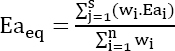
NOTE.– It can be seen that the “equivalent” activation energy is expressed as the arithmetic mean of various activation energies.
- – It can also be seen that the “equivalent” pre-exponential constant of the Arrhenius law is expressed as the geometric mean of various pre-exponential constants.
EXAMPLE.– Consider the data in Table 5.5.
Table 5.5. Value of C and Ea parameters for different manufacturers

Figure 5.17 is obtained.
Manufacturer weightings
Using a more realistic approach, it can also be considered that product designers do not use the components uniformly in terms of manufacturers. In other terms, some manufacturers are used more often than others. In this case, a “weighted” geometric mean can be defined as follows:

Figure 5.17. Example of global failure rates for manufacturers of components
Based on equations [5.13] and [5.16], we obtain:

with

Demonstration

End
EXAMPLE.– Let us resume the data of the previous example and add the following weights to Table 5.6.
Table 5.6. Values of C and Ea parameters for different manufacturers and associated weight

Figure 5.18 is obtained.

Figure 5.18. Global weighted failure rate of manufacturers