
3
Non-Regression Tests
This chapter aims to verify whether the new definitions of products, subsets or components are at least as good as the previous ones. As already noted, two cases are possible.
3.1. Non-regression on a physical quantity
The assumption made here is that the two definitions can be modeled by normal distribution. This point must be reinforced by a test of normality. To compare two samples of observations, the classical approach involves using a central tendency measure, which is generally the mean. Therefore, a comparison of two means will be made.
The two underlying hypotheses are:

To illustrate the proposed method, let us consider the data in Table 3.1.
First, a test of normality should be conducted on the two variables (see Figures 3.2 and 3.3).
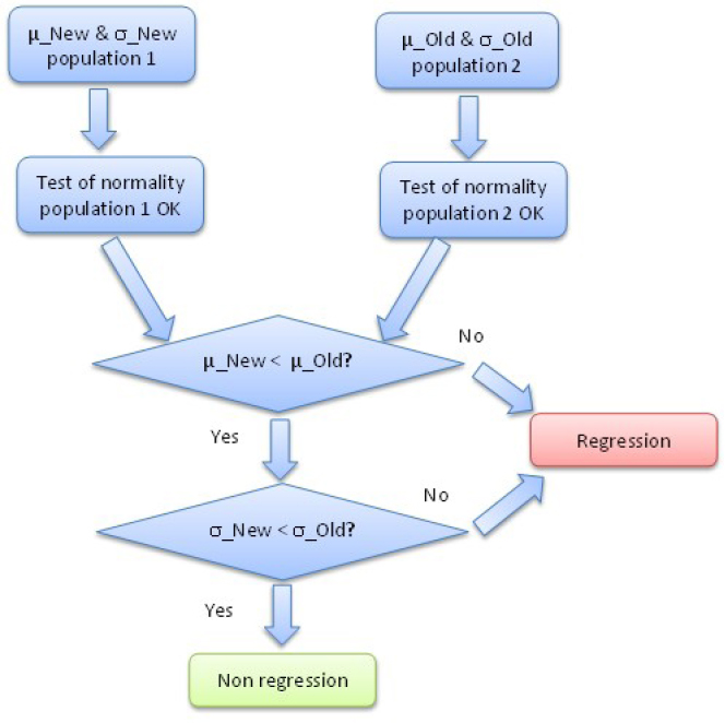
Figure 3.1. Overview diagram of non-regression on a physical quantity
Table 3.1. Example of a non-regression test
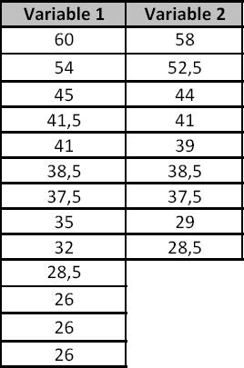

Figure 3.2. Test of normality on variable 1
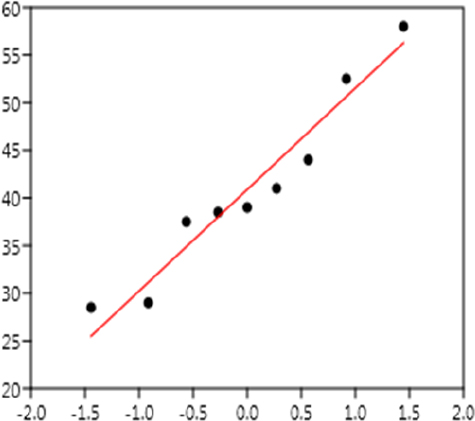
Figure 3.3. Test of normality on variable 2
The Anderson–Darling test yields a p-value of 47.9% and 36.4% for variables 1 and 2, respectively. Consequently, the hypothesis according to which the two variables are normal is not rejected, at a risk of 5%.
NOTE.– Other tests can be used (Shapiro, Lilliefors, etc.), but the conclusion is identical for all tests.
The equality of variances should be verified to compare the means. For this purpose, a Fisher test (or F-test) is used, and a statistic can be built based on the ratio of two variances according to a Fisher law.
For our example, this yields a p-value of ~ 73%. Therefore, the hypothesis of equality of variances is not called into question. Finally, a Student test (or t-test) can be used to compare the means of the two samples. This is a parametric test whose statistic t is given by:

where:
- – n1 is the size of the sample of population 1;
- – n2 is the size of the sample of population 2;
- –
 is the mean of data of population 1;
 - –
 is the mean of data of population 2;
 - –
 is the standard deviation of data of population 1;
 - –
 is the standard deviation of data of population 2.
It can be proven that this statistic follows Student’s law. Our example yields a p-value of ~ 49% and therefore the hypothesis of the equality of means is not called into question.
3.2. Non-regression depending on time
This section proposes the use of a method that compares the survival distributions of two definitions. A non-parametric test is proposed to avoid the estimation of the parameters of a model of accelerated reliability. The test that compares the survival distribution, known as the “log-rank test”, is what we are looking for (see Figure 3.4).
NOTE.– This test is non-parametric and therefore avoids the difficulty of estimating the parameters of a model, particularly that it can be accelerated.
- – Wrongly rejecting a new design is reflected by an improvement of the design, therefore useless additional costs are avoided.
- – Similarly, wrongly accepting non-regression is reflected in operations by unplanned additional costs and a strong degradation of the brand image in relation to the customer.
- – This test is the optimum in terms of costs since it can be stopped as soon as a significant difference between the two designs is noted.
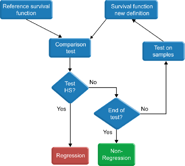
Figure 3.4. Diagram of a non-regression test
This test relies on the hypothesis that the two survival distributions are identical. As an illustration, let us consider the following example.
A test was conducted on a reference design, with 20 parts tested, with the following results:

A non-regression test was then conducted on a new definition, with eight parts tested, with the following results:
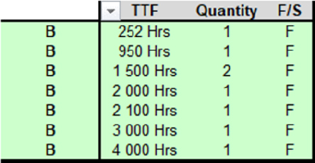
The graphical representation is presented in Figure 3.5.

Figure 3.5. Example of a non-regression test
The log-rank test shows that the survival distributions are different, and there is a regression in terms of reliability for the new design.