1
Sampling in Manufacturing
Chapters 1 to 6 of Volume 1 described various methods for building maturity. However, from a manufacturing perspective, these methods must be cost-effective. One of the solutions that can be considered to reduce costs is to test less than 100% of the products before delivery to the system manufacturer. This is called sampling.
As expected, there are various standards dealing with this subject, such as ISO 28590. These standards clarify the sampling rules to be applied, and the interested reader is invited to read them for further details.
However, the standards do not cover several aspects that are very important for the manufacturer:
- – The cost aspect, which leads to the following questions:
- - What is the benefit of applying a sampling rule?
- - Is a sampling rule adapted for my application?
- - What rule should I use to minimize costs?
- – What is the impact of test coverage rates if they are not 100%?
- – What is the impact of considering a distribution of potential defects?
This chapter aims to suggest a solution for each of these cases in order to formulate optimum sampling in terms of quality and cost.
Theoretically speaking, sampling techniques rely on discrete probability distributions (the random variable can only take certain values), unlike the probability distributions for estimating the reliability of a failure mechanism, which are continuous (e.g. exponential, Weibull, etc.). The Bernoulli distribution is used for the result of a test (failure or success). When this test is repeated several times, two cases are possible.
- – The “draw” is unrestricted, and in this case the binomial distribution is applicable.
- – The “draw” is restricted, and in this case the hypergeometric distribution is applicable.
Sampling is obviously a “restricted” draw. Therefore, the theoretical basis of the sampling norms is the hypergeometric distribution.
1.1. Cost aspects
The function of “cost associated with a size n sampling” is a random variable (the batch is accepted or rejected). Therefore, its average value (mathematical expectation) is considered here.
Given:
- – C is the cost per unit of the non-compliance test;
- – K is the cost per unit of accepting a non-compliant product in a batch;
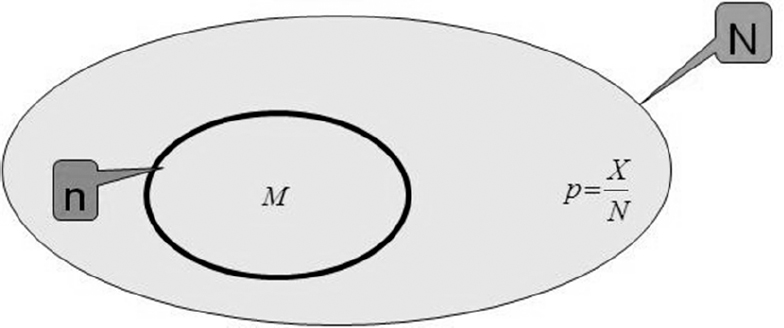
- – N is the number of products to be tested;
- – X is the number of “non-compliant” products in the batch;
- – n is the size of the sample.
The average cost is equal to the cost of compliant products plus the cost of non-compliant products. The cost of compliant products (if the batch was accepted) is given by:
P1 is the probability of having “no non-compliant parts” in a size “n” sample, randomly drawn from a batch of size “N”. Therefore it is:
where ![]() is the number of combinations of x out of y elements.
is the number of combinations of x out of y elements.
It is worth considering the details of this result. The probability of an event can be estimated by the ratio of the number of possible cases to the total number of cases. It is clear that the total number of cases is equal to the number of combinations of “n” taken out of “N”, or ![]()
The number of possible cases is equal to the number of combinations of compliant parts, or N–X, and is therefore equal to ![]() hence the result of equation [1.2].
hence the result of equation [1.2].
The cost of non-compliant products (if the batch was rejected) is given by:
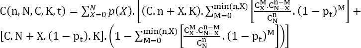
Based on equations [1.1], [1.2] and [1.3], the total cost is:
As an illustration, assume that:
- – there are 100 products to be delivered → N = 100;
- – the cost of a compliant part is C = 30€;
- – the cost of a non-compliant part is K = 1,500€.
According to this data, the cost of a non-compliant part is very high compared to the cost of a compliant part. Let us now consider the evolution of the total average cost depending on the size (n) and the number of defective products (X) (see Figure 1.1).
It can be noted that starting with X > 1, the sampling rate of 100% is optimal. In this example, the sampling is not interesting in terms of cost.
Now assume that:
- – there are 100 products to be delivered → N = 100;
- – the cost of a compliant part is C = 1,000€;
- – the cost of a non-compliant part is K = 1,500€.
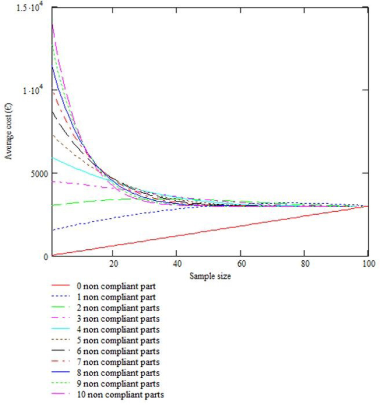
Figure 1.1. Evolution of the total average cost depending on the size of the sample and the number of defective products
Although low, the cost of a compliant part is of the order of the cost of non-compliant parts. Let us now consider the evolution of the total average cost depending on the sample size (n) and the number of defective products (X) (see Figure 1.2).
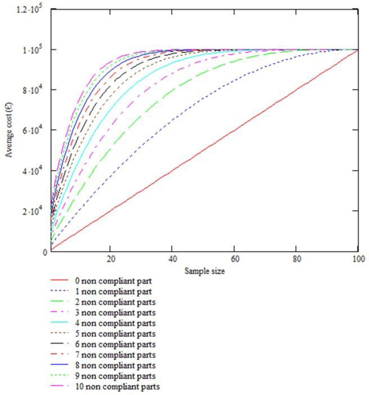
Figure 1.2. Evolution of the total average cost depending on the size of the sample and the number of defective products
In contrast to the previous example, in this case the sampling is better than the test at 100%.
Now assume that:
- – there are 100 products to be delivered → N = 100;
- – the cost of a compliant part is C = 100€;
- – the cost of a non-compliant part is K = 1,500€.
Let us now consider the evolution of the total average cost depending on the sample size (n) and the number of defective products (X) (see Figure 1.3).
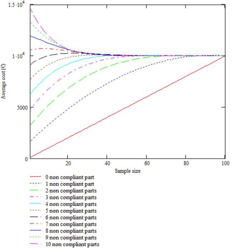
Figure 1.3. Evolution of the total average cost depending on the size of the sample and the number of defective products
This situation is an intermediate one between the two previously mentioned examples, as the sampling is optimal when the number of defects is equal to or greater than 7.
1.2. Considering the distribution of defects
Given p(X), the probability density of the defects observed during this phase of the test, the mathematical expectation of the cost is:
If this distribution is not known, the uniform probability distribution can be used:
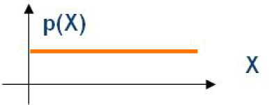
Given that the number of non-compliant products ranges between 0 and N, the probability density is then:
Using equations [10.5] and [10.6], the mathematical expectation of the cost is given by:
Once again, as an illustration, let us resume the following example and assume that:
- – there are 100 products to be delivered → N = 100;
- – the cost of a compliant part is C = 30€;
- – the cost of a non-compliant part is K = 1,500€.
Let us now consider the evolution of the total average cost depending on the sample size (n) (see Figure 1.4).
It can be noted that for a small sample size, the “average” cost can be very high.
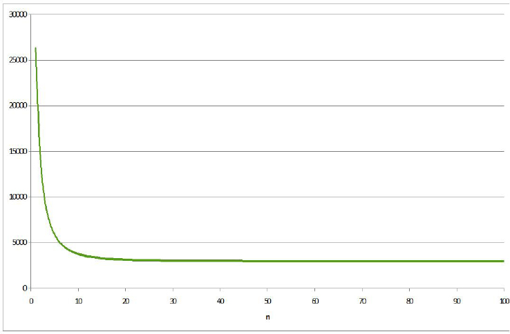
Figure 1.4. Evolution of the total average cost depending on the sample size – Example 1
Assume that:
- – there are 100 products to be delivered → N = 100;
- – the cost of a compliant part is C = 100€;
- – the cost of a non-compliant part is K = 1,500€.
Let us now examine the evolution of the total average cost depending on the sample size (n) (see Figure 1.5).
It can be noted that for a small sample size, the “average” cost can be very high. However, a slight optimum is obtained for n = 20, or a sampling rate of 20%, in this example.
Assume that:
- – there are 100 products to be delivered → N = 10;
- – the cost of a compliant part is C = 1,000€;
- – the cost of a non-compliant part is K = 1,500€.
Let us now examine the evolution of the total average cost depending on the sample size (n) (see Figure 1.6).
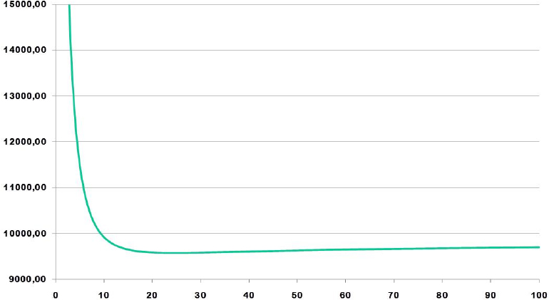
Figure 1.5. Evolution of the total average cost depending on the sample size – Example 2
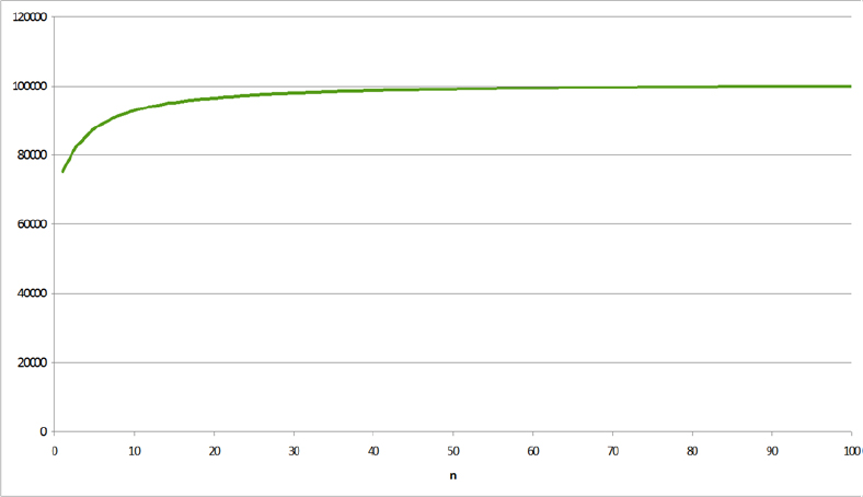
Figure 1.6. Evolution of the total average cost depending on the sample size – Example 3
It can be noted that for a small sample size, the “average” cost is the lowest.
1.3. Considering the test coverage
Given Pt, the probability of detecting a non-compliant product for a test, knowing that it will be detected by the client, let us denote by pnMNXt the probability of having M “non-compliant” parts in a sample of size n, drawn from a batch of size N, in which X parts are non-compliant.
Here, the number of possible cases is the number of possibilities of drawing M defective parts from X and drawing “n–M” compliant parts from the “N–X” compliant parts of the batch. The probability pnMNXt is then written as (hypergeometric distribution):
where ![]() is the number of possibilities of having defective products among the X products from the batch of size
is the number of possibilities of having defective products among the X products from the batch of size ![]() is the number of possibilities of having compliant products in the size n sample among the compliant parts of the batch, and
is the number of possibilities of having compliant products in the size n sample among the compliant parts of the batch, and ![]() is the number of possibilities of having n products among the N products.
is the number of possibilities of having n products among the N products.
The probability of detecting no non-compliant products in the M non-compliant products drawn in the test sampling is:
Finally, let us denote by pn0NXt the probability of having no non-compliant parts detected in a sample of size n, drawn in a batch of size N, in which X parts are non-compliant. Hence, according to the formula of total probabilities:
or, based on equations [1.9] and [1.10]:
Let us denote by Xd the number of parts detected as non-compliant when all the parts are tested following the rejection of the batch, as a result of the detection of at least one non-compliant part in a sample of size n. The “cost” function associated with a sample of size n, knowing that Xd non-compliant parts were detected, is defined as follows:
Since Xd follows a binomial law and E[Xd] = X.pt, the average cost depending on X is:
where ![]() is the additional cost due to the lack of detection capacity of tests pt. The cost depends on X number of non-compliant products in the batch, unknown by definition. Given p(X), the probability law of X for X = 0 to N, the expectation of the total cost of a test of n parts is therefore:
is the additional cost due to the lack of detection capacity of tests pt. The cost depends on X number of non-compliant products in the batch, unknown by definition. Given p(X), the probability law of X for X = 0 to N, the expectation of the total cost of a test of n parts is therefore: