
6
Efficient Model Training
Similar to how we scaled up data processing pipelines in the previous chapter, we can reduce the time it takes to train deep learning (DL) models by allocating more computational resources. In this chapter, we will learn how to configure the TensorFlow (TF) and PyTorch training logic to utilize multiple CPU and GPU devices on different machines. First, we will learn how TF and PyTorch support distributed training without any external tools. Next, we will describe how to utilize SageMaker, since it is built to handle the DL pipeline on the cloud from end to end. Lastly, we will look at tools that have been developed specifically for distributed training: Horovod, Ray, and Kubeflow.
In this chapter, we’re going to cover the following main topics:
- Training a model on a single machine
- Training a model on a cluster
- Training a model using SageMaker
- Training a model using Horovod
- Training a model using Ray
- Training a model using Kubeflow
Technical requirements
You can download the supplemental material for this chapter from this book’s GitHub repository: https://github.com/PacktPublishing/Production-Ready-Applied-Deep-Learning/tree/main/Chapter_6.
Training a model on a single machine
As described in Chapter 3, Developing a Powerful Deep Learning Model, training a DL model involves extracting meaningful patterns from a dataset. When the size of the dataset is small and the model has few parameters to tune, a central processing unit (CPU) might be sufficient to train the model. However, DL models have shown greater performance when they are trained with a larger training set and consist of a greater number of neurons. Therefore, training using a graphics processing unit (GPU) has become the standard since you can exploit its massive parallelism in matrix multiplication.
Utilizing multiple devices for training in TensorFlow
TF provides the tf.distribute.Strategy module, which allows you to use multiple GPU or CPU devices for training with very simple code modifications (https://www.tensorflow.org/guide/distributed_training). tf.distribute.Strategy is fully compatible with tf.keras.Model.fit, as well as custom training loops, as described in the Implementing and training a model in TensorFlow section of Chapter 3, Developing a Powerful Deep Learning Model. Various components of Keras, including variables, layers, models, optimizers, metrics, summaries, and checkpoints, are designed to support various tf.distribute.Strategy classes, keeping the transition to distributed training as simple as possible. Let’s have a look at how the tf.distribute.Strategy module allows you to quickly modify a set of code designed for a single device to multiple devices on a single machine:
import tensorflow as tf
mirrored_strategy = tf.distribute.MirroredStrategy()
# or
# mirrored_strategy = tf.distribute.MirroredStrategy(devices=["/gpu:0", "/gpu:1", "/gpu:3"])
# if you want to use only specific devices
with mirrored_strategy.scope():
    # define your model
    # …
model.compile(... )
model.fit(... )
Once the model has been saved, it can be loaded with or without the tf.distribute.Strategy scope. To achieve distributed training with a custom training loop, you can follow the example presented at https://www.tensorflow.org/tutorials/distribute/custom_training. Having said that, let’s review the most used strategies. We will cover the most common approaches, some of which go beyond training a single instance. They will be used in the next few sections, which cover training on multiple machines:
- Strategies that provide full support for tf.keras.Model.fit and custom training loops:
- MirroredStrategy: Synchronous distributed training using multiple GPUs on a single machine
- MultiWorkerMirroredStrategy: Synchronous distributed training on multiple machines (potentially using multiple GPUs per machine). This strategy class requires a TF cluster that’s been configured using the TF_CONFIG environment variable (https://www.tensorflow.org/guide/distributed_training#TF_CONFIG)
- TPUStrategy: Training on multiple tensor processing units (TPUs)
- Strategies with experimental features (meaning that classes and methods are still in the development stage) for tf.keras.Model.fit and custom training loops:
- ParameterServerStrategy: Model parameters are shared across multiple workers (the cluster consists of workers and parameter servers). Workers read and update the variables that are created on parameter servers after each iteration.
- CentralStorageStrategy: Variables are stored in central storage and replicated across each GPU.
- The last strategy that we want to mention is tf.distribute.OneDeviceStrategy (https://www.tensorflow.org/api_docs/python/tf/distribute/OneDeviceStrategy). It runs the training code on a single GPU device as follows:
strategy = tf.distribute.OneDeviceStrategy(device="/gpu:0")
In the preceding example, we have selected the first GPU ("/gpu:0").
It is also worth mentioning that the tf.distribute.get_strategy function can be used to get the current tf.distribute.Strategy object. You can use this function to change the tf.distribute.Strategy object dynamically for your training code, as shown in the following code snippet:
if tf.config.list_physical_devices('GPU'):
    strategy = tf.distribute.MirroredStrategy()
else:  # Use the Default Strategy
    strategy = tf.distribute.get_strategy()
In the preceding code, we are using tf.distribute.MirroredStrategy when GPU devices are available and fall back to the default strategy when GPU devices are not available. Next, let’s look at the features provided by PyTorch.
Utilizing multiple devices for training in PyTorch
To train a PyTorch model successfully, the model and input tensor need to be configured for the same device. If you want to use a GPU device, they need to be loaded on the target GPU device explicitly before training, using either the to(device=torch.device('cuda')) or cuda() function:
cpu = torch.device(cpu')
cuda = torch.device('cuda')     # Default CUDA device
cuda0 = torch.device('cuda:0')
x = torch.tensor([1., 2.], device=cuda0)
# x.device is device(type='cuda', index=0)
y = torch.tensor([1., 2.]).cuda()
# y.device is device(type='cuda', index=0)
# transfers a tensor from CPU to GPU 1
a = torch.tensor([1., 2.]).cuda()
# a.device are device(type='cuda', index=1)
# to function of a Tensor instance can be used to move the tensor to different devices
b = torch.tensor([1., 2.]).to(device=cuda)
# b.device are device(type='cuda', index=1)
The preceding example shows some of the key operations you should be aware of when using a GPU device. This is a subset of what is presented in the official PyTorch documentation: https://pytorch.org/docs/stable/notes/cuda.html.
However, setting up individual components for training can be tiresome. Therefore, PyTorch Lightning (PL) has decided to manage this automatically behind the scenes. In the case of PL, target devices can be chosen at the time of training, through the gpus parameter of Trainer:
# Train using CPU
Trainer()
# Specify how many GPUs to use
Trainer(gpus=k)
# Specify which GPUs to use
Trainer(gpus=[0, 1])
# To use all available GPUs put -1 or '-1'
Trainer(gpus=-1)
In the preceding example, we are describing various training setups for a single machine: training only using CPU devices, training using a set of GPU devices, and training using all GPU devices.
Things to remember
a. TF and PyTorch provide built-in support for training a model using both CPU and GPU devices.
b. Training can be controlled using the tf.distribute.Strategy class in TF. When training a model with a single machine, you can use MirroredStrategy or OneDeviceStrategy.
c. To train a PyTorch model using GPU devices, the model and relevant tensors need to be loaded on the same GPU device manually. PL hides most of the boilerplate code by handling the placements as part of the Trainer class.
In this section, we learned how to utilize multiple devices on a single machine. However, there have been many efforts to utilize a cluster of machines for training as there is a limit on the computational power that a single machine can have.
Training a model on a cluster
Even though using multiple GPUs on a single machine has reduced the training time a lot, some models are extremely huge and still require multiple days for training. Adding more GPUs is still an option but physical limitations often exist, preventing you from utilizing the full potential of the multi-GPU setting: motherboards can support a limited number of GPU devices.
Fortunately, many DL frameworks already support training a model on a distributed system. While there are minor differences in the actual implementation, most frameworks adopt the idea of model parallelism and data parallelism. As shown in the following diagram, model parallelism distributes components of the model to multiple machines, while data parallelism distributes the samples of the training set:

Figure 6.1 – The difference between model parallelism and data parallelism
There are a couple of details that you must be aware of when setting up a distributed system for model training. First, the machines in the cluster need to have a stable connection to the internet since they communicate over the network. If stability is not guaranteed, the cluster must have a way to recover from the connection issue. Ideally, the distributed system should be agnostic to the available machines and be able to add or remove a machine without affecting the overall progress. Such functionality will allow users to increase or decrease the number of machines dynamically, achieving the model training in the most cost-efficient way. AWS provides the aforementioned functionalities out of the box through Elastic MapReduce (EMR) and Elastic Container Service (ECS).
In the next two sections, we will take a deeper look into model parallelism and data parallelism.
Model parallelism
In the case of model parallelism, each machine in a distributed system takes a part of the model and manages computations for the assigned components. This approach is often considered when a network is too big to fit on a single GPU. However, it is not that common in reality because GPU devices often have enough memory to fit the model, and it is quite complex to set it up. In this section, we are going to describe the two most basic approaches of model parallelism: model sharding and model pipelining.
Model sharding
Model sharding is nothing more than partitioning the model into multiple computational subgraphs across multiple devices. Let’s assume a simple scenario of a basic single-tier deep neural network (DNN) model (no parallel paths). The model can be split into a few consecutive subgraphs, and the sharding profile can be graphically represented as follows. The data will flow sequentially starting from the device with the first subgraph. Each device will pass the computed values to the device of the next subgraph. Until the necessary data arrives, the devices will stay idle. In this example, we have four subgraphs:

Figure 6.2 – A sample distribution of a model in model sharding; each arrow indicates a mini-batch
As you can see, model sharding does not utilize the full computational resources; a device is waiting for the other device to process its subgraph. To solve this problem, the pipelining approach is proposed.
Model pipelining
In the case of model pipelining, a mini-batch is split into micro-batches and provided to the system in chains, as shown in the following diagram:
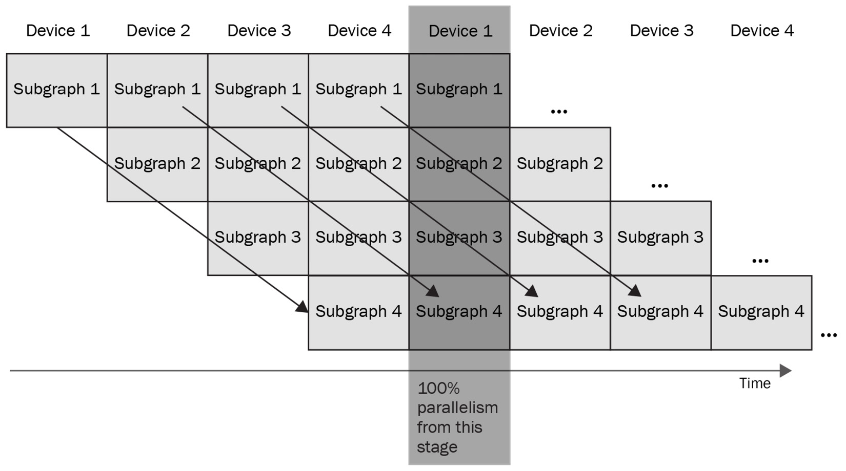
Figure 6.3 – A diagram of model pipeline logic; each arrow indicates a mini-batch
However, model pipelining requires a modified version of backward propagation. Let’s look at how a single forward and backward propagation can be achieved in a model pipelining setting. At some point, each device needs to perform not only forward computations for its subgraph but also gradient computations. A single forward and backward propagation can be achieved like so:

Figure 6.4 – A single forward and backward propagation in model pipelining
In the preceding diagram, we can see that each device runs forward propagation one by one and backward propagation in reverse order, passing the computed values to the next device. Putting everything together, we get the following diagram, which summarizes the logic of model pipelining:

Figure 6.5 – Model parallelism based on model pipelining
To further improve the training time, each device stores the values it computed previously and utilizes them in the following computations.
Model parallelism in TensorFlow
The following code snippet shows how to assign a set of layers to a specific device in TF as you define the model architecture:
with tf.device('GPU:0'):
    layer1 = layers.Dense(16, input_dim=8)
with tf.device('GPU:1'):
    layer2 = layers.Dense(4, input_dim=16)
If you want to explore model parallelism in TF even more, we recommend checking out the Mesh TF repository (https://github.com/tensorflow/mesh).
Model parallelism in PyTorch
Model parallelism is only available on PyTorch and has not yet been implemented in PL. While there are many ways to achieve model parallelism with PyTorch, the most standard approach is to use the torch.distributed.rpc module which achieves the communication among the machines using a remote procedure call (RPC). The three main features of the RPC-based approaches are triggering functions or networks remotely (remote execution), accessing and referencing remote data objects (remote reference), and extending the gradients update functionality of PyTorch across the machine boundaries (distributed gradients update). We delegate the details to the official documentation: https://pytorch.org/docs/stable/rpc.html.
Data parallelism
Data parallelism, unlike model parallelism, aims to speed up the training by sharding the dataset to the machines in the cluster. Each machine gets a copy of the model and computes the gradients with the dataset it has been assigned to. Then, the gradients are aggregated and the models are updated globally at once.
Data parallelism in TensorFlow
Data parallelism can be realized in TF by leveraging tf.distribute.MultiWorkerMirroredStrategy, tf.distribute.ParameterServerStrategy, and tf.distribute.CentralStorageStrategy.
We introduced these strategies in the Utilizing multiple devices for training in TensorFlow section since specific tf.distributed strategies are also used to set up training on multiple devices within a single machine.
To use these strategies, you need to set up a TF cluster where each machine can communicate with the other.
Typically, a TF cluster is defined using a TF_CONFIG environment variable. TF_CONFIG is just a JSON string that specifies cluster configuration by defining two components: cluster and task. The following Python code shows how to generate a .json file for TF_CONFIG from a Python dictionary:
tf_config = {
    'cluster': {
        'worker': ['localhost:12345', 'localhost:23456']
    },
    'task': {'type': 'worker', 'index': 0}
}
js_tf = json.dumps(tf_config)
with open("tf_config.json", "w") as outfile:
    outfile.write(js_tf)
The TF_CONFIG fields and formats are described at https://cloud.google.com/ai-platform/training/docs/distributed-training-details.
As demonstrated in the Utilizing multiple devices for training in TensorFlow section, you need to put the training code under the tf.distribute.Strategy scope. In the following example, we will show a sample usage for tf.distribute.MultiWorkerMirroredStrategy class.
First of all, you must put your model instance under the scope of tf.distribute.MultiWorkerMirroredStrategy, as shown in the following code snippet:
strategy = tf.distribute.MultiWorkerMirroredStrategy()
with strategy.scope():
    model = …
Next, you need to make sure the TF_CONFIG environment variables have been set up correctly for each machine in the cluster and run the training script, as follows:
# On the first node
TF_CONFIG='{"cluster": {"worker": ['localhost:12345', 'localhost:23456']}, "task": {"index": 0, "type": "worker"}}' python training.py
# On the second node
TF_CONFIG='{"cluster": {"worker": ['localhost:12345', 'localhost:23456']}, "task": {"index": 1, "type": "worker"}}' python training.py
To correctly save your model, please take a look at the official documentation: https://www.tensorflow.org/tutorials/distribute/multi_worker_with_keras.
In the case of a custom training loop, you can follow the instructions at https://www.tensorflow.org/tutorials/distribute/multi_worker_with_ctl.
Data parallelism in PyTorch
Unlike model parallelism, data parallelism is available for both PyTorch and PL. Among the various implementations, the most standard feature is torch.nn.parallel.DistributedDataParallel (DDP). In this section, we will mainly discuss PL as its main advantage comes from the simplicity of the training models that use data parallelism.
To train a model using data parallelism, you need to modify the training code to utilize the underlying distributed system and spawn a process with the torch.distributed.run module on each machine (https://pytorch.org/docs/stable/distributed.html).
The following code snippet describes what you need to change for ddp. You simply need to provide ddp for the accelerator parameter of Trainer. num_nodes is the parameter to adjust when there is more than one machine in the cluster:
# train on 8 GPUs (same machine)
trainer = Trainer(gpus=8, accelerator='ddp')
# train on 32 GPUs (4 nodes)
trainer = Trainer(gpus=8, accelerator='ddp', num_nodes=4)
Once the script has been set up, you need to run the following command on each machine. Please keep in mind that MASTER_ADDR and MASTER_PORT must be consistent as they are used by each processor to communicate. On the other hand, NODE_RANK indicates the index of the machine. In other words, it must be different for each machine, and it must start from zero:
python -m torch.distributed.run
--nnodes=2 # number of nodes you'd like to run with
--master_addr <MASTER_ADDR>
--master_port <MASTER_PORT>
--node_rank <NODE_RANK>
train.py (--arg1 ... train script args...)
Based on the official documentation, DDP works as follows:
- Each GPU across each node spins up a process.
- Each process gets a subset of the training set.
- Each process initializes the model.
- Each process performs both forward and backward propagation in parallel.
- The gradients are synchronized and averaged across all processes.
- Each process updates the weights of the model it has.
Things to remember
a. TF and PyTorch provide options for training DL models across multiple machines using model parallelism and data parallelism.
b. Model parallelism splits the model into multiple components and distributes them across machines. To set up model parallelism in TF and PyTorch, you can use the Mesh TensorFlow library and the torch.distributed.rpc package, respectively.
c. Data parallelism copies the model to each machine and distributes mini-batches across machines for training. In TF, data parallelism can be achieved using either MultiWorkerMirroredStrategy, ParameterServerStrategy, or CentralStorageStrategy. The main package that’s been designed for data parallelism in PyTorch is called torch.nn.parallel.DistributedDataParallel.
In this section, we learned how to achieve model training where the lifetime of the cluster is explicitly managed. However, some tools manage the clusters for model training as well. Since each of them has different advantages, you should understand the difference to select the right tool for your development.
First, we will look at the built-in features of SageMaker that train a DL model in a distributed fashion.
Training a model using SageMaker
As mentioned in the Utilizing SageMaker for ETL section of Chapter 5, Data Preparation in the Cloud, the motivation of SageMaker is to help engineers and researchers focus on developing high-quality DL pipelines without worrying about infrastructure management. SageMaker manages data storage and computational resources for you, allowing you to utilize a distributed system for model training with minimal effort. In addition, SageMaker supports streaming data to your models for inferencing, hyperparameter tuning, and tracking experiments and artifacts.
SageMaker Studio is the place where you define the logic for your model. The SageMaker Studio notebooks allow you to quickly explore the available data and set up model training logic. When model training takes too long, scaling up to use multiple computational resources and finding the best set of hyperparameters can be efficiently achieved by making a few modifications to the infrastructure’s configuration. Furthermore, SageMaker supports hyperparameter tuning on a distributed system to exploit parallelism.
Even though SageMaker sounds like a magic key for a DL pipeline, there are disadvantages as well. The first is its cost. Instances that have been allocated to SageMaker are around 40% more expensive than equivalent EC2 instances. Next, you may find that not all the libraries are available in the notebook. In other words, you may need to spend some additional time building and installing the library you need.
Setting up model training for SageMaker
By now, you should be able to start a notebook and select a predefined development environment for your project since we covered these in the Utilizing SageMaker for ETL section of Chapter 5, Data Preparation in the Cloud. Assuming that you have already processed raw data and stored the processed data in a data storage, we will focus on model training in this section. Model training with SageMaker can be summarized into the following three steps:
- If the processed data in the storage hasn’t been split into training, validation, and test sets yet, you must split them first.
- You need to define the model training logic and specify the cluster configuration.
- Lastly, you need to train your model and save the artifacts back in data storage. When training is completed, the allocated instances will be terminated automatically.
The key for model training with SageMaker is sagemaker.estimator.Estimator. It allows you to configure the training settings, including infrastructure setup, type of Docker images to use, and hyperparameters (https://sagemaker.readthedocs.io/en/stable/api/training/estimators.html). The following are the main parameters that you would typically configure:
- role (str): An AWS IAM role
- instance_count (int): The number of SageMaker EC2 instances to use for training
- instance_type (str): The type of SageMaker EC2 instance to use for training
- volume_size (int): The size of the Amazon Elastic Block Store (EBS) volume (in gigabytes) that will be used to download input data temporarily for training
- output_path (str): An S3 object where the training result will be stored
- use_spot_instances (bool): A flag specifying whether to use SageMaker-managed AWS Spot instances for training
- checkpoint_s3_uri (str): An S3 URI where the checkpoints will be stored during training
- hyperparameters (dict): A dictionary containing the initial set of hyperparameters
- entry_point (str): The path to the Python file to run
- dependencies (list[str]): A list of directories that will be loaded into the job
So long as you select the right container from Amazon Elastic Container Registry (ECR), you can set up any training configuration for SageMaker. Containers with various configurations for CPU and GPU devices also exist. You can find these at https://github.com/aws/deep-learning-containers/blob/master/available_images.md.
In addition, there exist repositories of open sourced toolkits designed to help TF and PyTorch model training on Amazon SageMaker. These repositories also contain Docker files that already have the necessary libraries installed, such as TF, PyTorch, and other dependencies necessary to build SageMaker images:
- TF: https://github.com/aws/sagemaker-tensorflow-training-toolkit
- PyTorch: https://github.com/aws/sagemaker-pytorch-training-toolkit
Lastly, we would like to mention that you can build and run the containers on your local machine. You can also update the installed libraries if you need to. If any modification is made, you need to upload the modified container to Amazon ECR before you can use it with sagemaker.estimator.Estimator.
In the following two sections, we will describe a set of changes that are required to train TF and PyTorch models.
Training a TensorFlow model using SageMaker
SageMaker provides a sagemaker.estimator.Estimator class built for TF: sagemaker.tensorflow.estimator.TensorFlow (https://sagemaker.readthedocs.io/en/stable/frameworks/tensorflow/sagemaker.tensorflow.html).
The following example shows the wrapper script that you need to write using the sagemaker.tensorflow.estimator.TensorFlow class to train a TF model on SageMaker:
import sagemaker
from sagemaker.tensorflow import TensorFlow
# Initializes SageMaker session
sagemaker_session = sagemaker.Session()
bucket = 's3://dataset/'
tf_estimator = TensorFlow(entry_point='training_script.py',
              source_dir='.',
              role=sagemaker.get_execution_role(),
              instance_count=1,
              instance_type='ml.c5.18xlarge',
              framework_version=tf_version,
              py_version='py3',
              script_mode=True,
              hyperparameters={'epochs': 30} )
Please keep in mind that every key in the hyperparameters parameter must have a corresponding entry defined in ArgumentParser of the training script (train_script.py). In the preceding example, we only have epochs defined ('epochs': 30).
To trigger the training, you need to call the fit function. You will need to provide datasets for training and validation. If you have them on an S3 bucket, the fit function will look as follows:
tf_estimator.fit({'training': 's3://bucket/training',
                  'validation': 's3://bucket/validation'})
The preceding example will run training_script.py, specified in the entry_point parameter, by locating it in the directory provided by source_dir. The details of the instance can be found in the instance_count and instance_type parameters. The training script will run with the parameters defined for hyperparameters of tf_estimator on the training and validation datasets defined in the fit function.
Training a PyTorch model using SageMaker
Similar to sagemaker.tensorflow.estimator.TensorFlow, there’s sagemaker.pytorch.PyTorch (). You can set up the training for your PyTorch (or PL) model, as described in the Implementing and training a model in PyTorch section of , Data Preparation in the Cloud, and integrate sagemaker.pytorch.PyTorch, as shown in the following code snippet:
import sagemaker
from sagemaker.pytorch import PyTorch
# Initializes SageMaker session
sagemaker_session = sagemaker.Session()
bucket = 's3://dataset/'
pytorch_estimator = PyTorch(
                      entry_point='train.py',
                      source_dir='.',
                      role=sagemaker.get_execution_role(),
                      framework_version='1.10.0',
                      train_instance_count=1,
                      train_instance_type='ml.c5.18xlarge',
                      hyperparameters={'epochs': 6})
…
pytorch_estimator.fit({
                        'training': bucket+'/training',
                        'validation': bucket+'/validation'})
The usage of a PyTorch estimator is identical to a TF estimator described in the previous section.
This concludes the basic usage of SageMaker for model training. Next, we will learn how to scale up training jobs in SageMaker. We will discuss distributed training using a distribution strategy. We will also cover how you can speed up the training by utilizing other data storage services that have lower latency.
Training a model in a distributed fashion using SageMaker
Data parallelism in SageMaker can be achieved using a distributed data parallel library (https://sagemaker.readthedocs.io/en/stable/api/training/smd_data_parallel.html).
All you need to do is to enable dataparallel as you create the sagemaker.estimator.Estimator instance, as follows:
distribution = {"smdistributed": {"dataparallel": { "enabled": True}} The following code snippet shows a TF estimator that’s been created with dataparallel. The full details can be found at https://docs.aws.amazon.com/en_jp/sagemaker/latest/dg/data-parallel-use-api.html:
tf_estimator = TensorFlow(
                 entry_point='training_script.py',
                 source_dir='.',
                 role=sagemaker.get_execution_role(),
                 instance_count=4,
                 instance_type='ml.c5.18xlarge',
                 framework_version=tf_version,
                 py_version='py3',
                 script_mode=True,
                 hyperparameters={'epochs': 30}
                 distributions={'smdistributed':
                 "dataparallel": {"enabled": True}})
The same modifications are necessary for a PyTorch estimator.
SageMaker supports two different mechanisms for transferring input data to the underlying algorithm: file mode and pipe mode. By default, SageMaker uses file mode, which downloads the input data to an EBS volume for training. However, if the amount of data is huge, this can slow down the training. In this case, you can use pipe mode, which streams data from S3 (using Linux FIFO) without making extra copies.
In the case of TF, you can simply use PipeModeDataset from the sagemaker-tensorflow extension (https://github.com/aws/sagemaker-tensorflow-extensions) as follows:
from sagemaker_tensorflow import PipeModeDataset
ds = PipeModeDataset(channel='training', record_format='TFRecord')
However, training a PyTorch model using pipe mode requires a bit more engineering effort. Therefore, we will point you to a notebook example that describes each step in depth: https://github.com/aws/amazon-sagemaker-examples/blob/main/advanced_functionality/pipe_bring_your_own/pipe_bring_your_own.ipynb.
The distributed strategy and pipe mode should speed up the training by scaling up the underlying computational resources and increasing the data transfer throughputs. However, if they are not sufficient, you can try leveraging two other more efficient data storage services that are compatible with SageMaker: Amazon Elastic File System (EFS) and Amazon fully managed shared storage (FSx) which was built for the Lustre filesystem. For more details, you can refer to their official pages at https://aws.amazon.com/efs/ and https://aws.amazon.com/fsx/lustre/, respectively.
SageMaker with Horovod
The other option for SageMaker distributed training is to use Horovod, a free and open source framework for distributed DL training based on Message Passing Interface (MPI) principles. MPI is a standard message-passing library that is widely used in parallel computing architectures. Horovod assumes that MPI is available for worker discovery and reduction coordination. Horovod can also utilize Gloo instead of MPI, an open source collective communications library. Here is an example of the distribution parameter configured for Horovod:
distribution={"mpi": {"enabled":True,
                        "processes_per_host":2 }}
In the preceding code snippet, we are achieving coordination among the machines using MPI. processes_per_host defines the number of processes to run on each instance. This is equivalent to defining the number of processes using the -H parameter in the mpirun or horovodrun command, which controls the program’s execution in MPI and Horovod, respectively.
In the following code snippet, we are selecting the number of parallel processes that control the number of training script executions (the -np parameter). Then, this number is split into specific machines using the specified values for the -H parameter. With the following commands, each machine will run train.py twice. This would be a typical setting when you have four machines with two GPUs each. The sum of assigned -H processes cannot exceed the -np value:
mpirun -np 8 -H server1:2,server2:2,server3:2,server4:2 … (other parameters) python train.py
We will discuss Horovod in depth in the following section as we cover how to train a DL model on a standalone Horovod cluster composed of EC2 instances.
Things to remember
a. SageMaker provides an excellent tool, SageMaker Studio, which allows you to quickly perform initial data exploration and train baseline models.
b. The sagemaker.estimator.Estimator object is an important component for training a model using SageMaker. It also supports distributed training on a set of machines with various CPU and GPU configurations.
c. Utilizing SageMaker for TF and PyTorch model training can be achieved estimators that are specifically designed for each framework.
Now, let’s look at how to use Horovod without SageMaker for distributed model training.
Training a model using Horovod
Even though we introduced Horovod as we introduced SageMaker, Horovod is designed to support distributed training alone (https://horovod.ai/). It aims to provide a simple way to train models in a distributed fashion by providing nice integrations for popular DL frameworks, including TensorFlow and PyTorch.
As mentioned previously in the SageMaker with Horovod section, the core principles of Horovod are based on MPI concepts such as size, rank, local rank, allreduce, allgather, broadcast, and alltoall (https://horovod.readthedocs.io/en/stable/concepts.html).
In this section, we will learn about how to set up a Horovod cluster using EC2 instances. Then, we will describe the modifications you need to make in TF and PyTorch scripts to train your model on the Horovod cluster.
Setting up a Horovod cluster
To set up a Horovod cluster using EC2 instances, you must follow these steps:
- Go to the EC2 instance console: https://console.aws.amazon.com/ec2/.
- Click the Launch Instances button in the top-right corner.
- Select Deep Learning AMI (the abbreviation for Amazon Machine Image) with TF, PyTorch, and Horovod installed. Click the Next … button at the bottom right.
- Select the right Instance Type for your training. You can select CPU or GPU instance types that fit your needs. Click the Next … button at the bottom right:

Figure 6.6 – Instance type selection in the EC2 Instance console
- Select the desired number of instances that will make up your Horovod cluster. Here, you can also request AWS Spot instances (cheaper instances based on the sparse EC2 capacity that can be interrupted, making them only feasible for fault-tolerant tasks). However, let’s use on-demand resources for simplicity.
- Select the right network and subnet settings. In real life, this type of information will be provided by the DevOps department.
- On the same page, select Add instance to placement group and Add to a new placement group, type the name that you want to use for the group, and select cluster for placement group strategy.
- On the same page, provide your Identity and Access Management (IAM) role so that you can access S3 buckets. Click the Next … button at the bottom right.
- Select the right storage size for your instances. Click the Next … button at the bottom right.
- Select unique labels/tags (https://docs.aws.amazon.com/general/latest/gr/aws_tagging.html) for your instances. In real life, these might be used as additional security measures, such as terminating instances with specific tags. Click the Next … button at the bottom right.
- Create a security group or choose an existing one. Again, you must talk to the DevOps department to get the proper information. Click the Next … button at the bottom right.
- Review all the information and launch. You will be asked to provide a Privacy Enhanced Mail (PEM) key for authentication.
After these steps, the desired number of instances will start up. If you didn’t add the Name tag in Step 10, your instances will not have any names. In this case, you can navigate to the EC2 Instances console and update the names manually. At the time of writing, you can request static IPv4 addresses called Elastic IPs and assign them to your instances (https://docs.aws.amazon.com/AWSEC2/latest/UserGuide/elastic-ip-addresses-eip.html).
Finally, you need to ensure that the instances can communicate with each other without an issue. You should check the Security Groups settings and add inbound rules for SSH and other traffic if necessary.
At this point, you just need to copy your PEM key from your local machine to the master EC2 instance. For an Ubuntu AMI, you can run the following command:
scp -i <your_pem_key_path> ubuntu@<IPv4_Public_IP>:/home/ubuntu/.ssh/
Now, you can use SSH to connect to the master EC2 instance. What you need to do next is to set the passwordless connections between EC2 instances by providing your PEM key in the SSH command using the following commands:
eval 'ssh-agent'
ssh-add <your_pem_key>
In the preceding code snippet, the eval command sets the environment variables provided by the ssh-agent command, while ssh-add command adds a PEM identity to the authentication agent.
Now, the cluster is ready to support Horovod! When you are finished, you must stop or terminate your cluster on the web console. Otherwise, it will continuously charge you for the resources.
In the next two sections, we will learn how to change the TF and PyTorch training scripts for Horovod.
Configuring a TensorFlow training script for Horovod
To train a TF model using Horovod, you need the horovod.tensorflow.keras module. First of all, you need to import the tensorflow and horovod.tensorflow.keras modules. We will refer to horovod.tensorflow.keras as hvd. Then, you need to initialize the Horovod cluster as follows:
import tensorflow as tf
import horovod.tensorflow.keras as hvd
# Initialize Horovod
hvd.init()
At this point, you can check the size of the cluster using the hvd.size function. Each process in Horovod will be assigned a rank (a number from 0 to the size of the cluster in terms of the processes you want to run or devices you want to use), which you can access through the hvd.rank function. On each instance, each process has a distinct number assigned from 0 to the number of processes on that instance, known as the local rank (the unique numbers per instance but duplicated across instances). The local rank for the current process can be accessed using the hvd.local_rank function.
You can pin a specific GPU device for each process using local rank as follows. This example also shows how to set memory growth for your GPUs using tf.config.experimental.set_memory_growth:
gpus = tf.config.experimental.list_physical_devices('GPU')
for gpu in gpus:
    tf.config.experimental.set_memory_growth(gpu, True)
if gpus:
    tf.config.experimental.set_visible_devices(gpus[hvd.local_rank()], 'GPU')
In the following code, we are splitting the data based on rank so that each process trains on a different set of examples:
dataset = np.array_split(dataset, hvd.size())[hvd.rank()]
For the model architecture, you can follow the instructions in the Implementing and training a model in TensorFlow section of Chapter 3, Developing a Powerful Deep Learning Model:
model = …
Next, you need to configure the optimizer. In the following example, the learning rate is scaled by the Horovod size. Also, the optimizer needs to be wrapped with a Horovod optimizer:
opt = tf.optimizers.Adam(0.001 * hvd.size())
opt = hvd.DistributedOptimizer(opt)
The next step is to compile your model and put the network architecture definition and optimizer together. When you are calling the compile function with a version of TF that’s older than v2.2, you need to disable experimental_run_tf_function so that TF uses hvd.DistributedOptimizer to compute gradients:
model.compile(loss=tf.losses.SparseCategoricalCrossentropy(),
              optimizer=opt,
              metrics=['accuracy'],
              experimental_run_tf_function=False)
Another component you need to configure is the callback function. You need to add hvd.callbacks.BroadcastGlobalVariablesCallback(0). This will broadcast the initial values of the weights and biases from rank 0 to all other machines and processes. This is necessary to ensure consistent initialization or to correctly restore training from a checkpoint:
callbacks=[
    hvd.callbacks.BroadcastGlobalVariablesCallback(0)
]
You can use rank to perform a particular operation on a specific instance. For example, logging and saving artifacts on a master node can be achieved by checking whether rank is 0 (hvd.rank()==0), as shown in the following code snippet:
# Save checkpoints only on the instance with rank 0 to prevent other workers from corrupting them.
If hvd.rank()==0:
    callbacks.append(keras.callbacks.ModelCheckpoint('./checkpoint-{epoch}.h5'))
Now, you are ready to trigger the fit function. The following example shows how to scale the number of steps per epoch using the size of the Horovod cluster. Messages from the fit function will be only visible on the master node:
if hvd.rank()==0:
    ver = 1
else:
    ver = 0
model.fit(dataset,
          steps_per_epoch=hvd.size(),
          callbacks=callbacks,
          epochs=num_epochs,
          verbose=ver)
This is all you need to change to train a TF model in a distributed fashion using Horovod. You can find the complete example at https://horovod.readthedocs.io/en/stable/tensorflow.html. The Keras version can be found at https://horovod.readthedocs.io/en/stable/keras.html. Additionally, you can modify your training script so that it runs in a fault-tolerant way: https://horovod.readthedocs.io/en/stable/elastic_include.html. With this change, you should be able to use AWS Spot instances and significantly decrease the cost of training.
Configuring a PyTorch training script for Horovod
Unfortunately, PL does not have proper documentation for Horovod support yet. Therefore, we will focus on PyTorch in this section. Similar to what we described in the preceding section, we will demonstrate the code change you need to make for the PyTorch training script. For PyTorch, you need the horovod.torch module, which we will refer to as hvd again. In the following code snippet, we are importing the necessary modules and initializing the cluster:
import torch
import horovod.torch as hvd
# Initialize Horovod
hvd.init()
As described in the TF example, you need to bind a GPU device for the current process using the local rank:
torch.cuda.set_device(hvd.local_rank())
The other parts of the training script require similar modifications. The dataset needs to be distributed across the instances using torch.utils.data.distributed.DistributedSampler and the optimizers must be wrapped around hvd.DistributedOptimizer. The major difference comes from hvd.broadcast_parameters(model.state_dict(), root_rank=0), which broadcasts the model weights. You can find the details in the following code snippet:
# Define dataset...
train_dataset = ...
# Partition dataset among workers using DistributedSampler
train_sampler = torch.utils.data.distributed.DistributedSampler(
    train_dataset, num_replicas=hvd.size(), rank=hvd.rank())
train_loader = torch.utils.data.DataLoader(train_dataset, batch_size=..., sampler=train_sampler)
# Build model...
model = ...
model.cuda()
optimizer = optim.SGD(model.parameters())
# Add Horovod Distributed Optimizer
optimizer = hvd.DistributedOptimizer(optimizer, named_parameters=model.named_parameters())
# Broadcast parameters from rank 0 to all other processes.
hvd.broadcast_parameters(model.state_dict(), root_rank=0)
Now, you are ready to train the model. The training loop does not require any modifications. You can just pass the input tensor to the model and trigger backward propagation by triggering the backward function on the loss and step function of optimizer. The following code snippet describes the main part of the training logic:
for epoch in range(num_ephos):
   for batch_idx, (data, target) in enumerate(train_loader):
       optimizer.zero_grad()
       output = model(data)
       loss = F.nll_loss(output, target)
       loss.backward()
       optimizer.step()
The complete description can be found on the official Horovod documentation page: https://horovod.readthedocs.io/en/stable/pytorch.html.
As the last piece of content for the Training model using Horovod section, the next section explains how to use the horovodrun and mpirun commands to initiate the model training process.
Training a DL model on a Horovod cluster
Horovod uses MPI principles to coordinate work between processes. To run four processes on a single machine, you can use one of the following commands:
horovodrun -np 4 -H localhost:4 python train.py
mpirun -np 4 python train.py
In both cases, the -np parameter defines the number of times the train.py script runs in parallel. The -H parameter can be used to define the number of processes per machine (see the horovodrun command in the preceding example). As we learn how to run on a single machine, -H can be dropped, as presented in the mpirun command. Other mpirun parameters are described at https://www.open-mpi.org/doc/v4.0/man1/mpirun.1.php#sect6.
If you do not have MPI installed, you can run the horovodrun command using Gloo. To run the same script to localhost four times (four processes) using Gloo, you just need to add the --gloo flag:
horovodrun --gloo -np 4 -H localhost:4 python train.py
Scaling up to multiple instances is quite simple. The following command shows how to run the training script on four machines using horovodrun:
horovodrun -np 4 -H server1:1,server2:1,server3:1,server4:1 python train.py
The following command shows how to run the training script on four machines using mpirun:
mpirun -np 4 -H server1:1,server2:1,server3:1,server4:1 python train.py
Once one of the preceding commands is triggered from the master node, you will see that each instance runs one process for training.
Things to remember
a. To use Horovod, you need a cluster with open cross-communication among the nodes.
b. Horovod provides a simple and effective way to achieve data parallelism for TF and PyTorch.
c. The training scripts can be executed on a Horovod cluster using the horovodrun or mpirun commands.
In the next section, we will describe Ray, another popular framework for distributed training.
Training a model using Ray
Ray is an open source execution framework for scaling Python workloads across machines (https://www.ray.io). The following Python workloads are supported by Ray:
- DL model training implemented with PyTorch or TF
- Hyperparameter tuning via Ray Tune (https://docs.ray.io/en/latest/tune/index.html)
- Reinforcement learning (RL) via RLlib (https://docs.ray.io/en/latest/rllib/index.html), an open source library for RL
- Data processing leveraging Ray Datasets (https://docs.ray.io/en/latest/data/dataset.html)
- Model serving via Ray Serve (https://docs.ray.io/en/latest/serve/index.html)
- A general Python application leveraging Ray Core (https://docs.ray.io/en/latest/ray-core/walkthrough.html)
The key advantage of Ray comes from the simplicity of its cluster definition; you can define a cluster with machines of different types and from various sources. For example, Ray allows you to build instance fleets (clusters based on a wide variety of EC2 instances with flexible and elastic resourcing strategies for each node) by mixing AWS EC2 on-demand instances and EC2 Spot instances with different CPU and GPU configurations. Ray simplifies both cluster creation and integration with DL frameworks, making it an effective tool for distributed DL model training processes.
First, we will learn how to set up a Ray cluster.
Setting up a Ray cluster
You can set up a Ray cluster in two ways:
- Ray Cluster Launcher: A tool provided by Ray to help build clusters using instances on cloud services, including AWS, GCP, and Azure
- Manual cluster construction: All the nodes need to be connected to the Ray cluster manually
A Ray cluster consists of a head node (master node) and worker nodes. The instances that form the cluster should be configured to communicate with each other over the network. Communication among Ray instances is based on a Transmission Control Protocol (TCP) connection, and you must have the corresponding ports open. In the next two sections, we will take a closer look at Ray Cluster Launcher and manual cluster construction.
Setting up a Ray cluster using Ray Cluster Launcher
A YAML file is used to configure the cluster when using Ray Cluster Launcher. You can find many sample YAML files for different configurations on Ray’s GitHub repository: https://github.com/ray-project/ray/tree/master/python/ray/autoscaler.
We will introduce the most basic one in this section. The YAML file starts with some basic information about the cluster, such as the name of the cluster, number of maximum workers, and upscaling speed, as follows:
cluster_name: BookDL
max_workers: 5
upscaling_speed: 1.0
Next, it configures the cloud service providers:
provider:
    type: aws
    region: us-east-1
    availability_zone: us-east-1c, us-east-1b, us-east-1a
    cache_stopped_nodes: True
    ssh_user: ubuntu
    ssh_private_key: /Users/BookDL/.ssh/BookDL.pem
In the preceding example, we specify the provider type (type: aws) and select the Region and Availability Zone where instances will be provided (region: us-east-1 and availability_zone: us-east-1c, us-east-1b, us-east-1a). Then, we define whether nodes can be reused in the future (cache_stopped_nodes: True). The last configurations are for user authentication (ssh_user:ubuntu and ssh_private_key:/Users/BookDL/.ssh/BookDL.pem).
Next, the node configuration needs to be specified. First of all, we will start with the head node:
available_node_types:
    ray.head.default:
        node_config:
            KeyName:"BookDL.pem"
Next, we must set up the security settings. The detailed settings must be consulted with DevOps, which monitors and secures the instances:
            SecurityGroupIds:
                - sg-XXXXX
                - sg-XXXXX
            SubnetIds: [subnet-XXXXX]
The following configurations are for the instance type and AMI that should be used:
            InstanceType: m5.8xlarge
            ImageId: ami-09ac68f361e5f4a13
In the following code snippet, we are providing configurations for storage:
            BlockDeviceMappings:
                  - DeviceName: /dev/sda1
                    Ebs:
                    VolumeSize: 580
You can easily define Tags as follows:
            TagSpecifications:
                - ResourceType:"instance"
                  Tags:
                      - Key:"Developer"
                        Value:"BookDL"
If needed, you can provide an IAM instance profile for accessing particular S3 buckets:
            IamInstanceProfile:
                Arn:arn:aws:iam::XXXXX
In the next section of the YAML file, we need to provide a configuration for worker nodes:
    ray.worker.default:
            min_workers: 2
            max_workers: 4
First of all, we must specify the number of workers (min_workers and max_workers). Then, we can define the node configuration similar to how we defined the master node configuration:
        node_config:
            KeyName: "BookDL.pem"
            SecurityGroupIds:
                - sg-XXXXX
                - sg-XXXXX
            SubnetIds: [subnet-XXXXX]
            InstanceType: p2.8xlarge
            ImageId: ami-09ac68f361e5f4a13
            TagSpecifications:
                - ResourceType: "instance"
                  Tags:
                      - Key: "Developer"
                        Value: "BookDL"
            IamInstanceProfile:
                Arn: arn:aws:iam::XXXXX
            BlockDeviceMappings:
              - DeviceName: /dev/sda1
                Ebs:
                  VolumeSize: 120
In addition, you can specify a list of shell commands to run on each node in the YAML file:
setup_commands:
    - (stat $HOME/anaconda3/envs/tensorflow2_p38/ &> /dev/null && echo 'export PATH="$HOME/anaconda3/envs/tensorflow2_p38/bin:$PATH"' >> ~/.bashrc) || true
    - source activate tensorflow2_p38 && pip install --upgrade pip
    - pip install awscli
    - pip install Cython
    - pip install -U ray
    - pip install -U ray[rllib] ray[tune] ray
    - pip install mlflow
    - pip install dvc
In this example, we will add tensorflow2_p38 for the conda environment to the path, activate the environment, and install a few other modules using pip. If you want to run some other commands just on the head or worker nodes, you can specify them in head_setup_commands and worker_setup_commands, respectively. They will be executed after the commands defined in setup_commands are executed.
Finally, the YAML file ends with commands for starting the Ray cluster:
head_start_ray_commands:
    - ray stop
    - source activate tensorflow2_p38 && ray stop
    - ulimit -n 65536; source activate tensorflow2_p38 && ray start --head --port=6379 --object-manager-port=8076 --autoscaling-config=~/ray_bootstrap_config.yaml
worker_start_ray_commands:
    - ray stop
    - source activate tensorflow2_p38 && ray stop
    - ulimit -n 65536; source activate tensorflow2_p38 && ray start --address=$RAY_HEAD_IP:6379 --object-manager-port=8076
At first, setting up a Ray cluster with a YAML file may look complex. However, once you are used to it, you will notice that adjusting cluster settings for future projects becomes rather simple. In addition, it reduces the time needed to spin up correctly defined clusters significantly as you may reuse information about security groups, subnets, tags, and IAM profiles from previous projects.
If you need other details, we recommend you spend some time looking at the official documentation: https://docs.ray.io/en/latest/cluster/config.html#cluster-config.
It is worth mentioning that Ray Cluster Launcher supports both autoscaling and using instance fleets with or without EC2 Spot instances. We used AMI in the preceding example, but you can also provide a specific Docker image for your instances. By exploiting the flexibility of the YAML configuration file, you can construct any cluster configurations using a single file.
As we mentioned at the beginning of this section, you can also set up a Ray cluster by manually adding individual instances. We’ll look at this option next.
Manually setting up a Ray cluster
Given that you have a set of machines with a network connection, the first step is to install Ray on each machine. Next, you need to change the security settings of each machine so that the machines can communicate with each other. After that, you need to select one node as a head node and run the following command:
ray start --head --redis-port=6379
The preceding command establishes the Ray cluster; the Redis server (used for the centralized control plane) is started, and its IP address gets printed on the terminal (for example, 123.45.67.89:6379).
Next, you need to run the following command on all the other nodes:
ray start --address=<redis server ip address>
The address you need to provide is the one that is printed from the command on the head node.
Now, your machines are ready to support Ray applications. In the manual setting case, the following steps need to be done manually: starting machines, connecting to a head node terminal, copying training files to all nodes, and stopping machines. Let’s have a look at how Ray Cluster Launcher can be utilized to help with those tasks.
At this stage, you should be able to specify the desired Ray cluster settings using a YAML file. Whenever you are ready, you can launch your first Ray cluster using the following command:
ray up your_cluster_setting_file.yaml
To get a remote terminal on the head node, you can run the following command:
ray attach your_cluster_setting_file.yaml
To terminate the cluster, the following command can be used:
ray down your_cluster_setting_file.yaml
Now, it’s time to learn how to perform DL model training on a Ray cluster.
Training a model in a distributed fashion using Ray
Ray provides the Ray Train library, which allows you to focus on defining training logic by handling the distributed training behind the scenes. Ray Train supports TF and PyTorch. It also provides simple integration with Horovod. In addition, Ray Datasets exists, which provides distributed data loading through distributed data transformations. Finally, Ray provides hyperparameter tuning through the Ray Tune library.
Adjusting TF training logic for Ray is similar to what we described in the Data parallelism in TensorFlow section. The main difference comes from the Ray Train library, which helps us set TF_CONFIG.
The adjusted training logic looks as follows:
def train_func_distributed():
    per_worker_batch_size = 64
    tf_config = json.loads(os.environ['TF_CONFIG'])
    num_workers = len(tf_config['cluster']['worker'])
    strategy = tf.distribute.MultiWorkerMirroredStrategy()
    global_batch_size = per_worker_batch_size * num_workers
    multi_worker_dataset = dataset(global_batch_size)
    with strategy.scope():
        multi_worker_model = build_and_compile_your_model()
    multi_worker_model.fit(multi_worker_dataset, epochs=20, steps_per_epoch=50)
Then, you can run the training with Ray Trainer, as follows:
import ray
from ray.train import Trainer
ray.init()
trainer = Trainer(backend="tensorflow", num_workers=4, use_gpu=True)
trainer.start()
trainer.run(train_func_distributed)
trainer.shutdown()
In the preceding example, the model definition is similar to a single device case, except that it should be compiled with a specific strategy: MultiWorkerMirroredStrategy. The dataset gets split inside the dataset function, providing a different set of samples for each worker node. Finally, the Trainer instance handles the distributed training.
Training PyTorch models using Ray can be achieved with a minimal set of changes as well. A few examples are presented at https://docs.ray.io/en/latest/train/examples.html#pytorch.
In addition, you can use Ray with Horovod, where you can leverage Elastic Horovod to train in a fault-tolerant way. Ray will autoscale the training process by simplifying the discovery and orchestration of hosts. We will not cover the details, but a good starting point can be found at https://docs.ray.io/en/latest/train/examples/horovod/horovod_example.html.
Things to remember
a. The key advantage of Ray comes from its simplicity of cluster definition.
b. A Ray cluster can be created manually by connecting each machine or using a built-in tool called Ray Cluster Launcher.
c. Ray provides a nice support for autoscaling the training process. It simplifies the discovery and orchestration of hosts.
Finally, let’s learn how to use Kubeflow for distributed training.
Training a model using Kubeflow
Kubeflow (https://www.kubeflow.org) covers every step of model development, including data exploration, preprocessing, feature extraction, model training, model serving, inferencing, and versioning. Kubeflow allows you to easily scale from a local development environment to production clusters by leveraging containers and Kubernetes, a management system for containerized applications.
Kubeflow might be your first choice for distributed training if your organization is already using the Kubernetes ecosystem.
Introducing Kubernetes
Kubernetes is an open source orchestration platform that’s used to manage containerized workloads and services (https://kubernetes.io):
- Kubernetes helps with continuous delivery, integration, and deployment.
- It separates development environments from deployment environments. You can construct a container image and develop the application in parallel.
- The container-based approach ensures the consistency of the environment for development, testing, as well as production. The environment will be consistent on a desktop computer or in the cloud, which minimizes the modifications necessary from one step to the other.
We assume that you have Kubeflow and all of its dependencies installed already, along with a running Kubernetes cluster. The steps we will describe in this section are generic enough that they can be used for any cluster settings – Minikube (a local version of Kubernetes), AWS Elastic Kubernetes Service (EKS), or a cluster of many nodes. This is the beauty of containerized workloads and services. The local Minikube installation steps can be found online at https://minikube.sigs.k8s.io/docs/start/. For EKS, we direct you to the AWS user guide: https://docs.aws.amazon.com/eks/latest/userguide/getting-started.html.
Setting up model training for Kubeflow
The first step is to package your training code into a container. This can be achieved with a Docker file. Depending on your starting point, you can use containers from the NVIDIA container image space (TF at https://docs.nvidia.com/deeplearning/frameworks/tensorflow-release-notes/running.html or PyTorch at https://docs.nvidia.com/deeplearning/frameworks/pytorch-release-notes/index.html) or containers directly from DL frameworks (TF at https://hub.docker.com/r/tensorflow/tensorflow or PyTorch at https://hub.docker.com/r/pytorch/pytorch).
Let’s have a look at an example TF docker file (kubeflow/tf_example_job):
FROM tensorflow/tensorflow:latest-gpu-jupyter
RUN pip install minio –upgrade
RUN pip install –upgrade pip
RUN pip install pandas –upgrade
…
RUN mkdir -p /opt/kubeflow
COPY train.py /opt/kubeflow
ENTRYPOINT ["python", "/opt/kubeflow/train.py"]
In the preceding Docker definition, the train.py script is a typical TF training script.
For now, we assume that a single machine will be used for training. In other words, it will be a single container job. Given that you have a Docker file and a training script prepared, you can build your container and push it to the repository using the following commands:
docker build -t kubeflow/tf_example_job:1.0
docker push kubeflow/tf_example_job:1.0
We will use TFJob, a custom component of Kubeflow that contains a custom resource descriptor (CRD) which defines how to use resources during training, and a controller which in our case, enables the TF library. TFJob is represented as a YAML file that describes the container image, the script for training, and execution parameters. Let’s have a look at a YAML file, tf_example_job.yaml, which contains a Kubeflow model training job running on a single machine:
apiVersion: "kubeflow.org/v1"
kind: "TFJob"
metadata:
    name: "tf_example_job"
spec:
    tfReplicaSpecs:
        Worker:
            replicas: 1
        restartPolicy: Never
        template:
            specs:
                containers:
                    - name: tensorflow
                      image: kubeflow/tf_example_job:1.0
The API version is defined in the first line. Then, the type of your custom resource is listed, kind: "TFJob". The metadata field is used to identify your job by giving it a custom name. The cluster is defined in the tfReplicaSpecs field. As shown in the preceding example, the script (tf_example_job:1.0) will be executed just once (replicas: 1).
To deploy the defined TFJob to your cluster, you can use the kubectl command, as follows:
kubectl apply -f tf_example_job.yaml
You can monitor your job with the following command (using the name defined in the metadata):
kubectl describe tfjob tf_example_job
To perform distributed training, you can use TF code with a specific tf.distribute.Strategy, create a new container, and modify TFJob. We will have a look at the necessary changes for TFJob in the next session.
Training a TensorFlow model in a distributed fashion using Kubeflow
Let’s assume that we already have the TF training code from MultiWorkerMirroredStrategy. For TFJob to support this strategy, you need to adjust tfReplicaSpecs in the spec field. We can define replicas of the following types through the YAML file:
- Chief (master): Orchestrates computational tasks
- Worker: Runs computations
- Parameter server: Manages storage for model parameters
- Evaluator: Runs evaluations during model training
As the simplest example, we will define a worker as one of those that can act as a chief node. Parameter server and evaluator are not obligatory.
Let's look at the adjusted YAML file, tf_example_job_dist.yaml, for the distributed TF training:
apiVersion: "kubeflow.org/v1"
kind: "TFJob"
metadata:
    name: "tf_example_job_dist"
spec:
    cleanPodPolicy: None
    tfReplicaSpecs:
        Worker:
            replicas: 4
            restartPolicy: Never
            template:
                specs:
                    containers:
                        - name: tensorflow
                          image: kubeflow/tf_example_job:1.1
The preceding YAML file will run the training job based on MultiWorkerMirroredStrategy on a new container, kubeflow/tf_example_job:1.1. We can deploy TFJob to the cluster with the same command:
kubectl apply -f tf_example_job_dist.yaml
In the next section, we will learn how to use PyTorch with Ray.
Training a PyTorch model in a distributed fashion using Kubeflow
For PyTorch, we just need to change TFJob to PyTorchJob and provide a PyTorch training script. For the training script itself, please refer to the Data parallelism in PyTorch section. The YAML file requires the same set of modifications, as shown in the following code snippet:
apiVersion: "kubeflow.org/v1
kind: "PyTorchJob"
metadata:
    name: "pt_example_job_dist"
spec:
    pytorchReplicaSpecs:
        Master:
            replicas: 1
            restartPolicy: Never
            template:
                specs:
                    containers:
                        - name: pytorch
                          image: kubeflow/pt_example_job:1.0
        Worker:
            replicas: 5
            restartPolicy: OnFailure
            template:
                specs:
                    containers:
                        - name: pytorch
                          image: kubeflow/pt_example_job:1.0
In this example, we have one master node and five replicas of worker nodes. The complete details can be found at https://www.kubeflow.org/docs/components/training/pytorch.
Things to remember
a. Kubeflow allows you to easily scale from a local development environment to large clusters leveraging containers and Kubernetes.
b. TFJob and PyTorchJob allow you to run TF and PyTorch training jobs in a distributed fashion using Kubeflow, respectively.
In this section, we described how to utilize Kubeflow for training TF and PyTorch models in a distributed fashion.
Summary
By realizing the benefit of parallelism that comes from multiple devices and machines, we have learned about various ways to train a DL model. First, we learned how to use multiple CPU and GPU devices on a single machine. Then, we covered how to utilize the built-in features of TF and PyTorch to achieve the training in a distributed fashion, where the underlying cluster is managed explicitly. After that, we learned how to use SageMaker for distributed training and scaling up. Finally, the last three sections described frameworks that are designed for distributed training: Horovod, Ray, and Kubeflow.
In the next chapter, we will cover model understanding. We will learn about popular techniques for model understanding that provide some insights into what is happening within the model throughout the training process.