3

Developing a Powerful Deep Learning Model

In this chapter, we will describe how to design and train a deep learning (DL) model. Within the notebook context described in the previous chapter, data scientists investigate various network designs and model training settings to generate a working model for the given task. The main topics of this chapter include the theory behind DL and how to train a model using the most popular DL frameworks: PyTorch and TensorFlow (TF). At the end of the chapter, we will decompose the StyleGAN implementation, a popular DL model for image generation, to explain how to construct a complex model using the components that we have introduced in this chapter.

In this chapter, we’re going to cover the following main topics:

• Going through the basic theory of DL
• Understanding the components of DL frameworks
• Implementing and training a model in PyTorch
• Implementing and training a model in TF
• Decomposing a complex, state-of-the-art model implementation

Technical requirements

You can download the supplemental material of this chapter from the following GitHub link: https://github.com/PacktPublishing/Production-Ready-Applied-Deep-Learning/tree/main/Chapter_3.

The samples in this chapter can be executed from any Python environment with the necessary packages installed. You can use the sample environment introduced in the last chapter: https://github.com/PacktPublishing/Production-Ready-Applied-Deep-Learning/tree/main/Chapter_2/dockerfiles.

Going through the basic theory of DL

As briefly described in Chapter 1, Effective Planning of Deep-Learning-Driven Projects, DL is a machine learning (ML) technique based on artificial neural networks (ANNs). In this section, our goal is to explain how ANNs work without going too deep into the math.

How does DL work?

An ANN is basically a set of connected neurons. As shown in Figure 3.1, neurons from an ANN and neurons from our brain behave in a similar way. Each connection in an ANN consists of a tunable parameter called the weight. When there is a connection from neuron A to neuron B, the output of neuron A gets multiplied by the weight of the connection; the weighted value becomes the input of neuron B. Bias is another tunable parameter within a neuron; a neuron sums up all the inputs and adds the bias. The last operation is an activation function that maps the computed value into a different range. The value in the new range is the output of the neuron, which gets passed to other neurons based on the connections.

Throughout the research, it has been found that groups of neurons captures different patterns based on their organization. Some of the powerful organizations are standardized as layers and have become the main building block for an ANN, providing a layer of abstraction on top of the complicated interactions among the neurons.

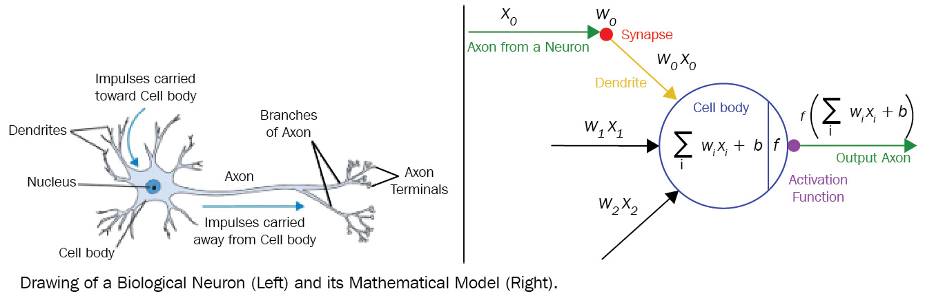
Figure 3.1 – A comparison of a biological neuron and a mathematical model of an ANN neuron

As described in the preceding diagram, operations in DL are based on numerical values. Therefore, the input data for a network must be converted into a numerical value. For example, a Red, Green, and Blue (RGB) color code is a standard way of representing an image using numerical values. In the case of text data, word embeddings are often used. Similarly, the output of a network will be a set of numerical values. The interpretation of these values can vary based on the task and the definition.

DL model training

Overall, training an ANN is a process of finding a set of weights, biases, and activation functions that enable the network to extract meaningful patterns from the data. Now, the next question would be the following: how do we find the right set of parameters? Many researchers have tried to solve this problem using various techniques. Out of all the trials, the most effective algorithm discovered is an optimization algorithm called gradient descent, an iterative process that finds the local or global minimum.

When training a DL model, we need to define a function that quantizes the difference between predictions and ground-truth labels as a numeric value called a loss. With a loss function clearly defined, we iteratively generate intermediate predictions, compute loss values, and update model parameters in the direction toward the minimum loss.

Given that the goal of optimization is to find the minimum loss, model parameters need to be updated based on the train set samples in the opposite direction of the gradient (see Figure 3.2). To compute the gradients, the network keeps track of the intermediate values computed during the prediction pass (forward propagation). Then, starting from the last layer, it computes the gradients for each parameter exploiting the chain rule (backward propagation). Interestingly, model performance and training time can differ a lot based on how the parameters get updated in each iteration. The different parameter updating rules are captured within the concept of optimizers. One of the main tasks in DL is to select the type of optimizer that produces the model with the best performance.

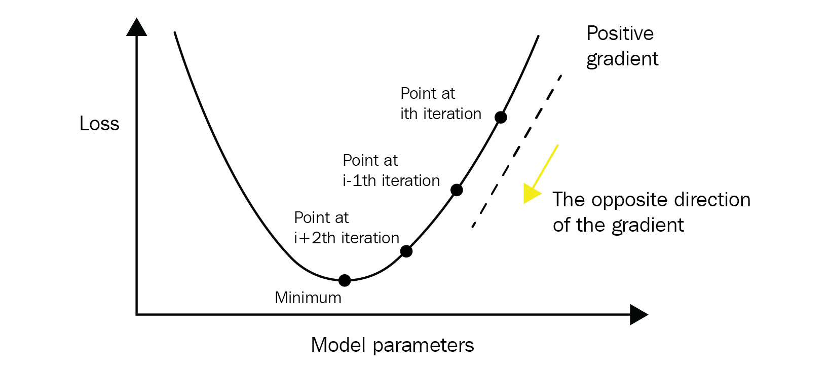
Figure 3.2 – With gradient descent, model parameters will be updated in the opposite direction of the gradient at every iteration

However, there is one caveat to this process. If the model is trained to achieve the best performance for the train set specifically, the performance on unseen data can possibly deteriorate. This is called overfitting; the model is trained specifically for the data it has seen before and fails to make correct predictions on new data. On the other hand, a shortage of training can lead to underfitting, a situation in which the model fails to capture the underlying pattern of the train set. To prevent these issues, a portion of the train set is put aside for evaluating the trained model throughout the training: the validation set. Overall, training for DL involves a process of updating the model parameters based on the train set but selecting the model that performs the best on the validation set. The last type of dataset, the test set, represents what the model would interact with once it is deployed. The test set may or may not be available at the time of model training. The purpose of the test set is to understand how the trained model would perform in production. To further understand the overall training logic, we can look at Figure 3.3:

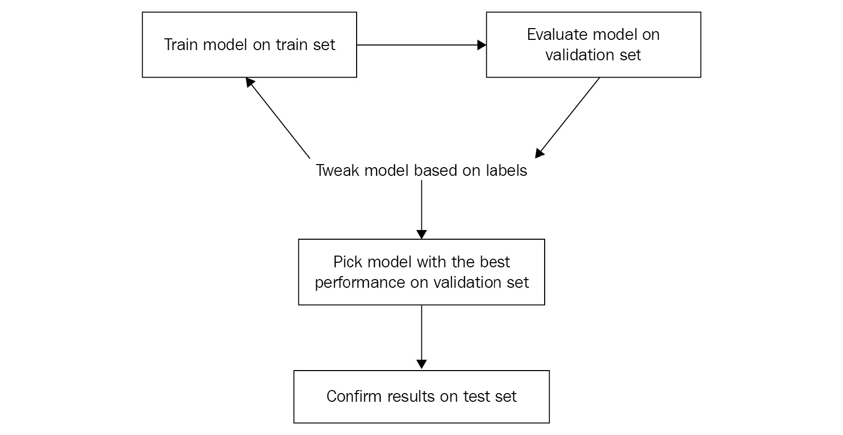
Figure 3.3 – The steps for training a DL model

The figure clearly describes what steps there are within the iterative process and what role each type of dataset plays in the scene.

Things to remember

a. Training an ANN is a process of finding a set of weights, biases, and activation functions that enable the network to extract meaningful patterns from the data.

b. There are three types of datasets in the training flow. The model parameters are updated using the train set, and the one that produces the best performance on the validation set is selected. The test set reflects the data distribution that the trained model would interact with upon deployment.

Next, we will look at DL frameworks that are designed to help us with model training.

Components of DL frameworks

Since the configuration of model training follows the same process regardless of the underlying tasks, many engineers and researchers have put together the common building blocks into frameworks. Most of the frameworks simplify DL model development by keeping data loading logic and model definitions independent from the training logic.

The data loading logic

Data loading logic includes everything from loading the raw data in memory to preparing each sample for training and evaluation. In many cases, data for the train set, validation set, and test set are stored in separate locations, so that each of them requires a distinct loading and preparation logic. The standard frameworks keep these logics separate from the other building blocks so that the model can be trained using different datasets in a dynamic way with minimal changes on the model side. Furthermore, the frameworks have standardized the way that these logics are defined to improve reusability and readability.

The model definition

Another building block, model definition, refers to the ANN architecture itself and corresponding forward and backward propagation logics. Even though building up a model using arithmetic operations is an option, the standard frameworks provide common layer definitions that users can put together to build up a complex model. Therefore, users are responsible for instantiating the necessary network components, connecting the components, and defining how the model should behave for training and inference.

In the following two sections, Implementing and training a model in PyTorch and Implementing and training a model in TF, we will introduce how to instantiate the popular layers in PyTorch and TF, respectively: dense (linear), pooling, normalization, dropout, convolution, and recurrent layers.

Model training logic

Lastly, we need to combine the two components and define the details of the training logic. This wrapper component must clearly describe the essential pieces of the model training, such as loss function, learning rate, optimizer, epochs, iterations, and batch size.

Loss functions can be classified into two major categories based on the type of learning task: classification loss and regression loss. The major difference between the two categories comes from the output format; the output of the classification task is categorical, while the output of the regression task is a continuous value. Out of the different losses, we will mainly discuss Mean Square Error (MSE) loss and Mean Absolute Error (MAE) loss for regression loss, and Cross-Entropy (CE) loss and Binary Cross-Entropy (BCE) loss for classification loss.

The learning rate (LR) defines the size of a step that gradient descent takes in the direction of the local minimum. Selecting the LR rate will help the process to converge faster, but if it’s too high or low, the convergence will not be guaranteed (see Figure 3.4):

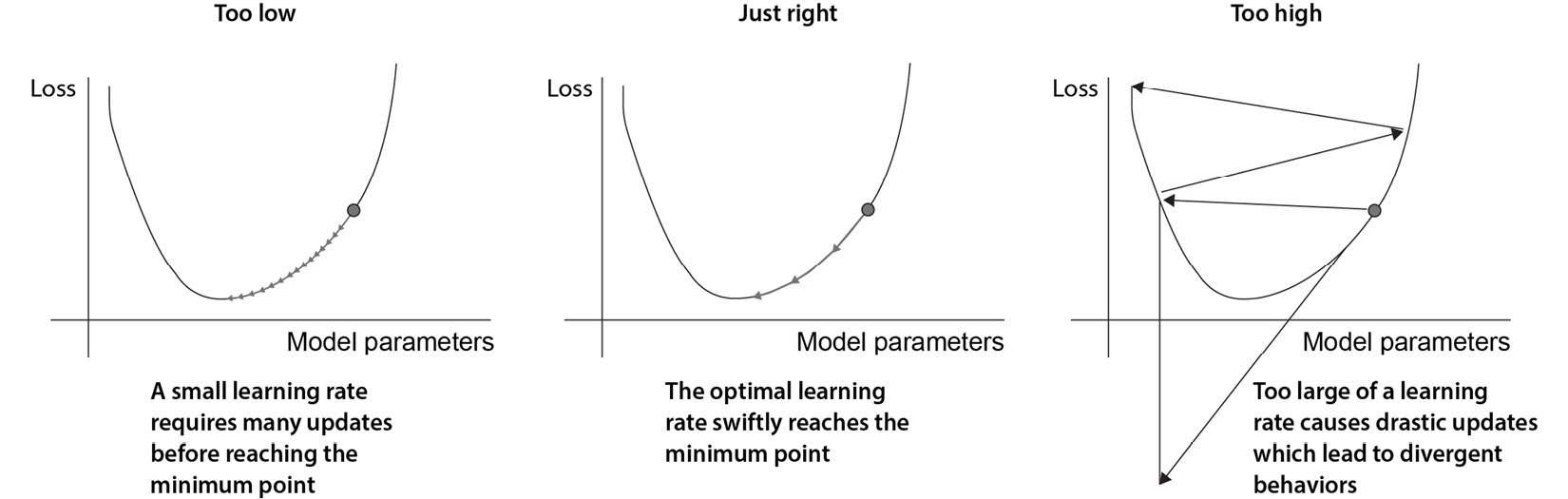
Figure 3.4 – The impact of the LR within gradient descent

Speaking of optimizers, we focus on the two main optimizers: Stochastic Gradient Descent (SGD), a basic optimizer with a fixed LR, and Adaptive Moment Estimation (Adam), an optimizer based on an adaptive LR that works the best in most scenarios. If you are interested in learning about different optimizers and the mathematics behind them, we recommend reading a survey paper by Choi et al (https://arxiv.org/pdf/1910.05446.pdf).

A single epoch indicates that every sample in the train set has been passed forward and backward through the network and that the network parameters have been updated. In many cases, the number of samples in the train set is way too huge to be passed through in one queue, so it gets divided into mini-batches. The batch size refers to the number of samples in a single mini-batch. Given that a set of mini-batches makes up the whole dataset, the number of iterations refers to the number of gradient update events (more precisely, the number of mini-batches) that model needs to interact with every sample. For example, if a mini-batch has 100 samples and there are 1,000 samples in total, it will require 10 iterations to complete one epoch. Selecting the right number of epochs is not an easy task. It changes depending on the other training parameters such as LR and batch size. Therefore, it often requires a trial-and-error process, keeping underfitting and overfitting in mind.

Things to remember

a. The components of model training can be broken down into data loading logic, model definition, and model training logic.

b. Data loading logic includes everything from loading raw data in the memory to preparing each sample for training and evaluation.

c. Model definition refers to the definition of the network architecture and its forward and backward propagation logics.

d. Model training logic handles the actual training by putting data loading logic and model definition together.

Out of the various frameworks available, we will discuss the two most popular in this book: TF and PyTorch. Keras running on TF has gained popularity in today, while PyTorch is heavily used for research with its exceptional flexibility and simplicity.

Implementing and training a model in PyTorch

PyTorch is a Python library for Torch, a ML package for Lua. The main features of PyTorch include graphics processing unit- (GPU-) accelerated matrix calculation and automatic differentiation for building and training neural networks. Creating the computation graph dynamically as the code gets executed, PyTorch is gaining popularity for its flexibility and ease of use, as well as its efficiency in model training.

Built on top of PyTorch, PyTorch Lightning (PL) provides another layer of abstraction, hiding many boilerplate codes. The new framework pays more attention to researchers by decoupling research-related components of PyTorch from the engineering-related components. PL codes are typically more scalable and easier to read than PyTorch codes. Even though the code snippets in this book put more emphasis on PL, PyTorch and PL share a lot of functionalities, so most components are interchangeable. If you are willing to dig into the details, we recommend the official site, https://pytorch.org.

There are other extensions of PyTorch available on the market:

• Skorch (https://github.com/skorch-dev/skorch) – A scikit-learn compatible neural network library that wraps PyTorch
• Catalyst (https://github.com/catalyst-team/catalyst) – A PyTorch framework specialized for reproducibility, rapid experimentation, and codebase reuse
• Fastai (https://github.com/fastai/fastai) – A library that standardizes not only high-level components for practitioners but also delivers low-level components for researchers
• PyTorch Ignite (https://pytorch.org/ignite/) – A library designed to help with training and evaluation for practitioners

We will not cover these libraries in this book, but you may find them helpful if you are new to this field.

Now, let’s dive into PyTorch and PL.

PyTorch data loading logic

For readability and modularity, PyTorch and PL exploit a class called Dataset for data management and another class, DataLoader, for accessing samples iteratively.

While the Dataset class handles fetching individual samples, model training takes in the input data in batches and requires reshuffling to reduce model overfitting. DataLoader abstracts this complexity for users by providing a simple API. Furthermore, it exploits Python’s multiprocessing features behind the scenes to speed up data retrieval.

The two core functions that must be implemented by the child class of Dataset are __len__ and __getitem__. As described in the following class outline, __len__ should return the total number of samples and __getitem__ should return a sample for the given index:

from torch.utils.data import Dataset
class SampleDataset(Dataset):
   def __len__(self):
      """return number of samples"""
   def __getitem__(self, index):
      """loads and returns a sample from the dataset at the given index"""

PL’s LightningDataModule encapsulates all the steps needed to process data. The key components include downloading and cleaning data, preprocessing each sample, and wrapping each type of dataset inside DataLoader. The following code snippet describes how to create a LightningDataModule class. The class has the prepare_data function for downloading and preprocessing the data, as well as three functions for instantiating DataLoader for each type of dataset, train_dataloader, val_dataloader, and test_dataloader:

from torch.utils.data import DataLoader
from pytorch_lightning.core.lightning import LightningDataModule
class SampleDataModule(LightningDataModule):
   def prepare_data(self):
       """download and preprocess the data; triggered only on single GPU"""
       ...
   def setup(self):
       """define necessary components for data loading on each GPU"""
       ...
   def train_dataloader(self):
       """define train data loader"""
       return data.DataLoader(
         self.train_dataset, 
           batch_size=self.batch_size, 
           shuffle=True)
   def val_dataloader(self):
       """define validation data loader"""
       return data.DataLoader(
          self.validation_dataset, 
          batch_size=self.batch_size, 
          shuffle=False)             
   def test_dataloader(self):
       """define test data loader"""
       return data.DataLoader(
          self.test_dataset, 
          batch_size=self.batch_size, 
          shuffle=False)

The official documentation for LightningDataModule can be found at https://pytorch-lightning.readthedocs.io/en/stable/extensions/datamodules.html.

PyTorch model definition

The key benefit of PL comes from LightningModule, which simplifies the organization of complex PyTorch codes into six sections:

• Computation (__init__)
• The train loop (training_step)
• The validation loop (validation_step)
• The test loop (test_step)
• The prediction loop (predict_step)
• Optimizers and LR scheduler (configure_optimizers)

The model architecture is part of the computation section. Necessary layers are instantiated inside the __init__ method, and computational logics are defined in the forward method. In the following code snippet, three linear layers are registered to the LightningModule module inside the __init__ method, and the relationships between them are defined inside the forward method:

from pytorch_lightning import LightningModule
from torch import nn
class SampleModel(LightningModule):
   def __init__(self):
      """instantiate necessary layers"""
       self.individual_layer_1 = nn.Linear(..., ...)
       self.individual_layer_2 = nn.Linear(..., ...)
       self.individual_layer_3 = nn.Linear(..., ...)
   def forward(self, input):
       """define forward propagation logic"""
       output_1 = self.individual_layer_1(input)
       output_2 = self.individual_layer_2(output_1)
       final_output = self.individual_layer_3(output_2)
       return final_output

Another way of defining a network is to use torch.nn.Sequential, as shown in the following code. With this module, a set of layers can be grouped together, and output chaining is automatically achieved:

class SampleModel(LightningModule):
   def __init__(self):
       """instantiate necessary layers"""
       self.multiple_layers = nn.Sequential(
       nn.Linear(    ,    ),
       nn.Linear(    ,    ),
       nn.Linear(    ,    ))
   def forward(self, input):
       """define forward propagation logic"""
       final_output = self.multiple_layers(input)
       return final_output

In the preceding code, the three linear layers are grouped together and stored as a single instance variable, self.multiple_layers. In the forward method, we simply trigger self.multiple_layers with the input tensor to pass the tensor through each layer one by one.

The following section is designed to introduce popular layer implementations.

PyTorch DL layers

One of the major benefits of DL frameworks comes from various layer definitions: gradient calculation logics are already part of the layer definitions, so you can focus on finding the best model architecture for your task. In this section, we will learn about layers that are commonly used across projects. Please refer to the official documentation (https://pytorch.org/docs/stable/nn.html) if the layer that you are interested in is not covered in this section.

PyTorch dense (linear) layer

The first type of layer is torch.nn.Linear. As the name suggests, it applies a linear transformation to the input tensor. The two main parameters of the function are in_features and out_features, which define the input and output tensor dimensions, respectively:

linear_layer = torch.nn.Linear(
              in_features,   # Size of each input sample
              out_features,  # Size of each output sample)
# N = batch size
# * = any number of additional dimensions
input_tensor = torch.rand(N, *, in_features)
output_tensor = linear_layer(input_tensor) # (N, *, out_features)

The layer implementation from the torch.nn module already has the forward function defined, so that you can use the layer variable as if it were a function to trigger forward propagation.

PyTorch pooling layers

Pooling layers are commonly used for downsampling a tensor. The two most popular types are maximum pooling and average pooling. The key parameters for these layers are kernel_size and stride, which define the size of the window and how it moves for each pooling operation.

The maximum pooling layer downsamples the input tensor by selecting the largest value for each window:

# 2D max pooling
max_pool_layer = torch.nn.MaxPool2d(
   kernel_size,         # the size of the window to take a max over
   stride=None,         # the stride of the window. Default value is kernel_size
   padding=0,           # implicit zero padding to be added on both sides
   dilation=1,          # a parameter that controls the stride of elements in the window)
# N = batch size
# C = number of channels
# H = height of input planes in pixels
# W = width of input planes in pixels
input_tensor = torch.rand(N, C, H, W)
output_tensor = max_pool_layer(input_tensor) # (N, C, H_out, W_out) 

On the other hand, the average pooling layer downsamples the input tensor by computing an average value for each window:

# 2D average pooling
avg_pool_layer = torch.nn.AvgPool2d(
   kernel_size,         # the size of the window to take a max over
   stride=None,         # the stride of the window. Default value is kernel_size
   padding=0,           # implicit zero padding to be added on both sides)
# N = batch size
# C = number of channels
# H = height of input planes in pixels
# W = width of input planes in pixels
input_tensor = torch.rand(N, C, H, W)
output_tensor = avg_pool_layer(input_tensor) # (N, C, H_out, W_out)

You can find the other types of pooling layers at https://pytorch.org/docs/stable/nn.html#pooling-layers.

PyTorch normalization layers

Commonly used in data processing, the purpose of normalization is to scale numerical data to a common scale without distorting the distribution. In the case of DL, normalization layers are used to train the network with greater numerical stability (https://pytorch.org/docs/stable/nn.html#normalization-layers).

The most popular normalization layer is the batch normalization layer, which scales a set of values in a mini-batch. In the following code snippet, we introduce torch.nn.BatchNorm2d, a batch normalization layer designed for a mini-batch of 2D tensors with an additional channel dimension:

batch_norm_layer = torch.nn.BatchNorm2d(
   num_features,      # Number of channels in the input image
   eps=1e-05,         # A value added to the denominator for numerical stability
   momentum=0.1,      # The value used for the running_mean and running_var computation
   affine=True,       # a boolean value that when set to True, this module has learnable affine parameters)
# N = batch size
# C = number of channels
# H = height of input planes in pixels
# W = width of input planes in pixels
input_tensor = torch.rand(N, C, H, W)
output_tensor = batch_norm_layer(input_tensor) # same shape as input (N, C, H, W)

Out of the various parameters, the main one that you should be aware of is num_features, which indicates the number of channels. The input to the layer is a 4D tensor, where each index indicates the batch size (N), number of channels (C), the height of the image (H), and the width of the image (W).

PyTorch dropout layer

The dropout layer helps the model to extract generic features by randomly setting a set of values to zero. This operation prevents the model from overfitting to the train set. Having said that, the dropout layer implementation of PyTorch mainly operates over a single parameter, p, which controls the probability of an element being zeroed:

drop_out_layer = torch.nn.Dropout2d(
   p=0.5,  # probability of an element to be zeroed )
# N = batch size
# C = number of channels
# H = height of input planes in pixels
# W = width of input planes in pixels
input_tensor = torch.rand(N, C, H, W)
output_tensor = drop_out_layer(input_tensor) # same shape as input (N, C, H, W)

In this example, we are dropping 50% of the elements (p=0.5). Similar to the batch normalization layer, the input tensor for torch.nn.Dropout2d has a size of N, C, H, W.

PyTorch convolution layers

Specialized for image processing, the convolutional layer is designed to apply convolution operations over the input tensor using a sliding window technique. In the case of image processing, where intermediate data is represented as 4D tensors of size N, C, H, W, torch.nn.Conv2d is the standard choice:

conv_layer = torch.nn.Conv2d(
   in_channels,         # Number of channels in the input image
   out_channels,        # Number of channels produced by the convolution
   kernel_size,         # Size of the convolving kernel
   stride=1,            # Stride of the convolution
   padding=0,           # Padding added to all four sides of the input.
   dilation=1,          # Spacing between kernel elements)
# N = batch size
# C = number of channels
# H = height of input planes in pixels
# W = width of input planes in pixels
input_tensor = torch.rand(N, C_in, H, W)
output_tensor = conv_layer(input_tensor) # (N, C_out, H_out, W_out)

The first parameter of the torch.nn.Conv2d class, in_channels, indicates the number of channels in the input tensor. The second parameter, out_channels, indicates the number of channels in the output tensor, which is equal to the number of filters. The other parameters, kernel_size, stride, and padding, determine how the convolution operations are carried out for the layer.

PyTorch recurrent layers

Recurrent layers are designed for sequential data. Among the various types of recurrent layers, we will cover torch.nn.RNN in this section, which applies a multi-layer Elman recurrent neural network (RNN) to the given sequence (https://onlinelibrary.wiley.com/doi/abs/10.1207/s15516709cog1402_1). If you would like to try different recurrent layers, you can refer to the official documentation: https://pytorch.org/docs/stable/nn.html#recurrent-layers:

# multi-layer Elman RNN with tanh or ReLU non-linearity to an input sequence.
rnn = torch.nn.RNN(
   input_size,                     # The number of expected features in the input x
   hidden_size,                    # The number of features in the hidden state h
   num_layers = 1,                 # Number of recurrent layers
   nonlinearity="tanh",            # The non-linearity to use. Can be either 'tanh' or 'relu'
   bias=True,                      # If False, then the layer does not use bias weights
   batch_first=False,              # If True, then the input and output tensors are provided
                                                                                                 # as (batch, seq, feature) instead of (seq, batch, feature)
             dropout=0,                                                # If non-zero, introduces a Dropout layer on the outputs of each RNN layer
                                                                                                 # except the last layer, with dropout probability equal to dropout
   bidirectional=False,             # If True, becomes a bidirectional RNN)
# N = batch size
# L = sequence length
# D = 2 if bidirectionally, otherwise 1
# H_in = input_size
# H_out = hidden_size
rnn = nn.RNN(H_in, H_out, num_layers)
input_tensor = torch.randn(L, N, H_in)
# H_0 = tensor containing the initial hidden state for each element in the batch
h0 = torch.randn(D * num_layers, N, H_out)
# output_tensor (L, N, D * H_out)
# hn (D * num_layers, N, H_out) 
output_tensor, hn = rnn(input_tensor, h0)

The three key parameters of torch.nn.RNN are input_size, hidden_size, and num_layers. They refer to the number of expected features in the input tensor, the number of features in the hidden state, and the number of recurrent layers to use, respectively. To trigger forward propagation, you need to pass two things, an input tensor and a tensor containing the initial hidden state.

PyTorch model training

In this section, we describe the model training component of PL. As shown in the following code block, LightningModule is the base class that you must inherit for this component. Its configure_optimizers function is used to define the optimizer for training. Then, the actual training logic is defined within the training_step function:

class SampleModel(LightningModule):
   def configure_optimizers(self):
      """Define optimizer to use"""
      return torch.optim.Adam(self.parameters(), lr=0.02)
   def training_step(self, batch, batch_idx):
      """Define single training iteration"""
      x, y = batch
      y_hat = self(x)
      loss = F.cross_entropy(y_hat, y)
      return loss

Validation, prediction, and the test loop have similar function definitions; a batch gets fed into the network to compute the necessary predictions and loss values. The collected data can also be stored and displayed using PL’s built-in logging system. For details, please refer to the official documentation (https://pytorch-lightning.readthedocs.io/en/latest/common/lightning_module.html):

   def validation_step(self, batch, batch_idx):
      """Define single validation iteration"""
      loss, acc = self._shared_eval_step(batch, batch_idx)
      metrics = {"val_acc": acc, "val_loss": loss}
      self.log_dict(metrics)
      return metrics
   def test_step(self, batch, batch_idx):
      """Define single test iteration"""
      loss, acc = self._shared_eval_step(batch, batch_idx)
      metrics = {"test_acc": acc, "test_loss": loss}
      self.log_dict(metrics)
      return metrics
   def _shared_eval_step(self, batch, batch_idx):
      x, y = batch
      outputs = self(x)
      loss = self.criterion(outputs, targets)
      acc = accuracy(outputs.round(), targets.int())
      return loss, acc
   def predict_step(self, batch, batch_idx, dataloader_idx=0):
      """Compute prediction for the given batch of data"""
      x, y = batch
      y_hat = self(x)
      return y_hat

Under the hood, LightningModule executes the following set of simplified PyTorch codes:

model.train()
torch.set_grad_enabled(True)
outs = []
for batch_idx, batch in enumerate(train_dataloader):
   loss = training_step(batch, batch_idx)
   outs.append(loss.detach())
   # clear gradients
   optimizer.zero_grad()
   # backward
   loss.backward()
   # update parameters
   optimizer.step()
   if validate_at_some_point
      model.eval()
      for val_batch_idx, val_batch in enumerate(val_dataloader):
         val_out = model.validation_step(val_batch, val_batch_idx)
         model.train()

Putting LightningDataModule and LightningModule together, the training and inference on the test set can be simply achieved as follows:

from pytorch_lightning import Trainer
data_module = SampleDataModule()
trainer = Trainer(max_epochs=num_epochs)
model = SampleModel()
trainer.fit(model, data_module)
result = trainer.test()

By now, you should’ve learned what you need to implement to set up a model training using PyTorch. The following two sections are dedicated to loss functions and optimizers, the two major components of model training.

PyTorch loss functions

First, we will look at the different loss functions available in PL. The loss functions in this sections can be found from the torch.nn module.

PyTorch MSE / L2 loss function

MSE loss function can be created using torch.nn.MSELoss. However, this calculates the square error component only and exploits the reduction parameter to provide variations. When reduction is None, the calculated value is returned as is. On the other hand, when it is set to sum, the outputs will be summed up. To obtain the exact MSE loss, the reduction must be set to mean, as shown in the following code snippet:

loss = nn.MSELoss(reduction='mean')
input = torch.randn(3, 5, requires_grad=True)
target = torch.randn(3, 5)
output = loss(input, target)

Next, let’s have a look at MAE loss.

PyTorch MAE / L1 loss function

MAE loss function can be instantiated using torch.nn.L1Loss. Similar to MSE loss function, this function calculates different values based on the reduction parameter:

Loss = nn.L1Loss(reduction='mean')
input = torch.randn(3, 5, requires_grad=True)
target = torch.randn(3, 5)
output = loss(input, target)

We can now move on to CE loss, which is used in multi-class classification tasks.

PyTorch CE loss functions

torch.nn.CrossEntropyLoss is useful when training a model for a classification problem with multiple classes. As shown in the following code snippet, this class also has a reduction parameter for calculating different variations. You can further change the behavior of the loss using weight and ignore_index parameters, which weight each class and ignore specific indices, respectively:

loss = nn.CrossEntropyLoss(reduction="mean")
input = torch.randn(3, 5, requires_grad=True)
target = torch.empty(3, dtype=torch.long).random_(5)
output = loss(input, target)

In a similar fashion, we can define BCE loss.

PyTorch BCE loss functions

Similar to CE loss, PyTorch defines the BCE loss as torch.nn.BCELoss with the same set of parameters. However, exploiting the close relationship between torch.nn.BCELoss and the sigmoid operation, PyTorch provides torch.nn.BCEWithLogitsLoss, which achieves higher numerical stability by combining the softmax operation and the BCE loss calculation in a single class. The usage is shown in the following code snippet:

loss = torch.nn.BCEWithLogitsLoss(reduction="mean")
input = torch.randn(3, requires_grad=True)
target = torch.empty(3).random_(2)
output = loss(input, target)

Finally, let’s have a look at construction of a custom loss in PyTorch.

PyTorch custom loss functions

Defining a custom loss function is straightforward. Any function defined with PyTorch operations can be used as a loss function.

The following is a sample implementation of torch.nn.MSELoss using the mean operator:

def custom_mse_loss(output, target):
   loss = torch.mean((output - target)**2)
   return loss
input = torch.randn(3, 5, requires_grad=True)
target = torch.randn(3, 5)
output = custom_mse_loss(input, target)

Now, we will move to the overview of optimizers in PyTorch.

PyTorch optimizers

As described in the PyTorch model training section, the configure_optimizers function of LightningModule specifies the optimizer for the training. In PyTorch, predefined optimizers can be found from the torch.optim module. The optimizer instantiation requires model parameters, which can be obtained by calling the parameters function on the model, as shown in the following sections.

PyTorch SGD optimizer

The following code snippet instantiates an SGD optimizer with an LR of 0.1 and demonstrates how a single step of a model parameter update can be achieved.

torch.optim.SGD has built-in support for momentum and acceleration, which further improves training performance. It can be configured using momentum and nesterov parameters:

optimizer = torch.optim.SGD(model.parameters(), lr=0.1 momentum=0.9, nesterov=True)

PyTorch Adam optimizer

Similarly, an Adam optimizer can be instantiated using torch.optim.Adam, as shown in the following line of code:

optimizer = torch.optim.Adam(model.parameters(), lr=0.1) 

If you are curious about how optimizers work in PyTorch, we recommend reading over the official documentation: https://pytorch.org/docs/stable/optim.html.

Things to remember

a. PyTorch is a popular DL framework that provides GPU-accelerated matrix calculation and automatic differentiation. PyTorch is gaining popularity for its flexibility, ease of use, as well as efficiency in model training.

b. For readability and modularity, PyTorch exploits a class called Dataset for data management and another class, DataLoader, for accessing samples iteratively.

c. The key benefit of PL comes from LightningModule, which simplifies the organization of the complex PyTorch code structure into six sections: computation, a train loop, validation loop, test loop, prediction loop, as well as optimizers and LR scheduler

d. PyTorch and PL share the torch.nn module for various layers and loss functions. Predefined optimizers can be found from the torch.optim module.

In the following section, we will look at another DL framework, TF. Training set up with TF is remarkably similar to the set up with PyTorch.

Implementing and training a model in TF

While PyTorch is oriented towards research projects, TF puts more emphasis on industry use cases. While the deployment features of PyTorch, Torch Serve, and Torch Mobile are still in the experimental phase, the deployment features of TF, TF Serve, and TF Lite are stable and actively in use. The first version of TF was introduced by the Google Brain team in 2011 and they have been continuously updating TF to make it more flexible, user-friendly, and efficient. The key difference between TF and PyTorch was initially much larger, as the first version of TF used static graphs. However, this situation has changed with version 2, as it introduces eager execution, mimicking dynamic graphs known from PyTorch. TF version 2 is often used with Keras, an interface for ANN (https://keras.io). Keras allows users to quickly develop DL models and run experiments. In the following sections, we will walk you through the key components of TF.

TF data loading logic

Data can be loaded for TF models in various ways. One of the key data manipulation modules that you should be aware of is tf.data, which helps you to build efficient input pipelines. tf.data provides tf.data.Dataset and tf.data.TFRecordDataset classes that are designed for loading datasets of different data formats. In addition, there are tensorflow_datasets (tfds) modules (https://www.tensorflow.org/datasets/api_docs/python/tfds) and tensorflow_addons modules (https://www.tensorflow.org/addons) that further simplify the data loading process in many cases. It is also worth mentioning the TF I/O package (https://www.tensorflow.org/io/overview), which expands the capabilities of the standard TF file system interaction.

Regardless of the package that you are going to use, you should consider creating a DataLoader class. In this class, you will clearly define how the target data will be loaded and how it will be preprocessed before the training. The following code snippet is a sample implementation with loading logic:

import tensorflow_datasets as tfds
class DataLoader: 
   """ DataLoader class"""
   @staticmethod 
   def load_data(config): 
      return tfds.load(config.data_url)

In the preceding example, we use tfds to load data from the external URL (config.data_url). More information about tfds.load can be found online: https://www.tensorflow.org/datasets/api_docs/python/tfds/load.

Data is available in various formats. Therefore, it is important that it is preprocessed into the format that TF models can consume using the functionalities provided by the tf.data module. So, let’s have a look at how to use this package for reading data of common formats:

• First, data in tfrecord, a format designed for storing a sequence of binary data, can be read as follows:

  import tensorflow as tf

  dataset = tf.data.TFRecordDataset(list_of_files)

• We can create a dataset object from a NumPy array using the tf.data.Dataset.from_tensor_slices function as follows:

  dataset = tf.data.Dataset.from_tensor_slices(numpy_array)

• Pandas DataFrames can also be loaded as a dataset using the same tf.data.Dataset.from_tensor_slices function:

  dataset = tf.data.Dataset.from_tensor_slices((df_features.values, df_target.values))

• Another option is to use a Python generator. Here is a simple example that highlights how to use a generator to feed a paired image and label:

  def data_generator(images, labels):

     def fetch_examples():

         i = 0

         while True:

            example = (images[i], labels[i])

            i += 1

            i %= len(labels)

            yield example

         return fetch_examples

  training_dataset = tf.data.Dataset.from_generator(

     data_generator(images, labels),

     output_types=(tf.float32, tf.int32),

     output_shapes=(tf.TensorShape(features_shape), tf.TensorShape(labels_shape)))

As shown in the last code snippet, tf.data.Dataset provides us with built-in data loading functionalities such as batching, repeating, and shuffling. These options are self-explanatory: batching creates mini-batches of a specific size, repeating allows us to iterate over dataset multiple times, and shuffling mixes up the data entries for every epoch.

Before we wrap up this section, we would like to mention that models implemented with Keras can directly consume NumPy arrays and Pandas DataFrames.

TF model definition

Similar to how PyTorch and PL handles model definition, TF provides various ways of defining network architecture. First, we will look at Keras.Sequential, which chains a set of layers to construct a network. This class handles the linkage for you so that you don’t need to define the linkage between the layers explicitly:

import tensorflow as tf
from tensorflow import keras
from tensorflow.keras import layers
input_shape = 50
model = keras.Sequential(
   [
      keras.Input(shape=input_shape),
      layers.Dense(128, activation="relu", name="layer1"),
      layers.Dense(64, activation="relu", name="layer2"),
      layers.Dense(1, activation="sigmoid", name="layer3"),
   ])

In the preceding example, we are creating a model that consists of an input layer, two dense layers, and an output layer that generates a single neuron as an output. This is a simple model that can be used for binary classification.

If the model definition is more complex and cannot be constructed in a sequential manner, another option is to use the keras.Model class, as shown in the following code snippet:

num_classes = 5 
input_1 = layers.Input(50)
input_2 = layers.Input(10)
x_1 = layers.Dense(128, activation="relu", name="layer1x")(input_1)
x_1 = layers.Dense(64, activation="relu", name="layer1_2x")(x_1)
x_2 = layers.Dense(128, activation="relu", name="layer2x")(input_2)
x_2 = layers.Dense(64, activation="relu", name="layer2_1x")(x_2)
x = layers.concatenate([x_1, x_2], name="concatenate")
out = layers.Dense(num_classes, activation="softmax", name="output")(x)
model = keras.Model((input_1,input_2), out)

In this example, we have two inputs with a distinct set of computations. The two paths are merged in the last concatenation layer, which transports the concatenated tensor into the final dense layer with five neurons. Given that the last layer uses softmax activation, this model can be used for multi-class classification.

The third option, as follows, is to create a class that inherits keras.Model. This option gives you the most flexibility, as it allows you to customize every part of the model and the training process:

class SimpleANN(keras.Model):
   def __init__(self):
      super().__init__()
      self.dense_1 = layers.Dense(128, activation="relu", name="layer1")
      self.dense_2 = layers.Dense(64, activation="relu", name="layer2")
      self.out = layers.Dense(1, activation="sigmoid", name="output")
   def call(self, inputs):
      x = self.dense_1(inputs)
      x = self.dense_3(x)
      return self.out(x)
model = SimpleANN()

SimpleANN, from the preceding code, inherits Keras.Model. Within the __init__ function, we need to define the network architecture using a tf.keras.layers module or basic TF operations. The forward propagation logic is defined inside a call method, just as PyTorch has the forward method.

When the model is defined as a distinct class, you can link additional functionalities to the class. In the following example, the build_graph method is added to return a keras.Model instance, so you can, for example, use the summary function to visualize the network architecture as a simpler representation:

class SimpleANN(keras.Model):
   def __init__(self):
   ...
   def call(self, inputs):
   ...
   def build_graph(self, raw_shape):
      x = tf.keras.layers.Input(shape=raw_shape)
      return keras.Model(inputs=[x], outputs=self.call(x))

Now, let’s look at how TF provides a set of layer implementations through Keras.

TF DL layers

As mentioned in the previous section, the tf.keras.layers module provides a set of layer implementations that you can use for building a TF model. In this section, we will cover the same set of layers that we described in the Implementing and training a model in PyTorch section. The complete list of layers available in this module can be found at https://www.tensorflow.org/api_docs/python/tf/keras/layers.

TF dense (linear) layers

The first one is tf.keras.layers.Dense, which performs a linear transformation:

tf.keras.layers.Dense(units, activation=None, use_bias=True, kernel_initializer='glorot_uniform', bias_initializer='zeros', kernel_regularizer=None, bias_regularizer=None, activity_regularizer=None, kernel_constraint=None, bias_constraint=None, **kwargs)

The units parameter defines the number of neurons in the dense layer (the dimensionality of the output). If the activation parameter is not defined, the output of the layer will be returned as is. As presented in the following code, we can apply an Activation operation outside of the layer definition as well:

X = layers.Dense(128, name="layer2")(input)
x = tf.keras.layers.Activation('relu')(x)

In some cases, you will need to build a custom layer. The following example demonstrates how to create a dense layer using basic TF operations by inheriting the tensorflow.keras.layers.Layer class:

import tensorflow as tf
from tensorflow.keras.layers import Layer
class CustomDenseLayer(Layer):
   def __init__(self, units=32):
      super(SimpleDense, self).__init__()
      self.units = units
   def build(self, input_shape):
      w_init = tf.random_normal_initializer()
      self.w = tf.Variable(name="kernel", initial_value=w_init(shape=(input_shape[-1], self.units),
      dtype='float32'),trainable=True)
      b_init = tf.zeros_initializer()
      self.b = tf.Variable(name="bias",initial_value=b_init(shape=(self.units,), dtype='float32'),trainable=True)
   def call(self, inputs):
      return tf.matmul(inputs, self.w) + self.b

Within the __init__ function of the CustomDenseLayer class, we define the dimensionality of the output (units). Then, the state of the layer is instantiated within the build method; we create and initialize the weights and biases for the layer. The last method, call, defines the computation itself. For a dense layer, it consists of multiplying the inputs with the weights and adding biases.

TF pooling layers

tf.keras.layers provides different kinds of pooling layers: average, max, global average, and global max pooling layers for one-dimensional temporal data, two-dimensional, or three-dimensional spatial data. In this section, we will show you two-dimensional max pooling and average pooling layers:

tf.keras.layers.MaxPool2D(
   pool_size=(2, 2), strides=None, padding='valid', data_format=None,
   kwargs)
tf.keras.layers.AveragePooling2D(
   pool_size=(2, 2), strides=None, padding='valid', data_format=None,
   kwargs)

The two layers both take in pool_size, which defines the size of the window. The strides parameter is used to define how the windows move throughout the pooling operation.

TF normalization layers

In the following example, we demonstrate a layer for batch normalization, tf.keras.layers.BatchNormalization:

tf.keras.layers.BatchNormalization(
   axis=-1, momentum=0.99, epsilon=0.001, center=True, scale=True,
   beta_initializer='zeros', gamma_initializer='ones',
   moving_mean_initializer='zeros',
   moving_variance_initializer='ones', beta_regularizer=None,
   gamma_regularizer=None, beta_constraint=None, gamma_constraint=None, **kwargs)

The output of this layer will have mean close to 0 and standard deviation close to 1. Details about each parameter can be found at https://www.tensorflow.org/api_docs/python/tf/keras/layers/BatchNormalization.

TF dropout layers

The Tf.keras.layers.Dropout layer applies dropout, a regularization method that sets randomly selected values to zero:

tf.keras.layers.Dropout(rate, noise_shape=None, seed=None, **kwargs)

In the preceding layer instantiation, the rate argument, a float value between 0 and 1, determines the fraction of the input units that will be dropped.

TF convolution layers

tf.keras.layers provides various implementations of convolutional layers, tf.keras.layers.Conv1D, tf.keras.layers.Conv2D, tf.keras.layers.Conv3D, and the corresponding transposed convolutional layers (deconvolution layers), tf.keras.layers.Conv1DTranspose, tf.keras.layers.Conv2DTranspose, and tf.keras.layers.Conv3DTranspose.

The following code snippet describes the instantiation of a two-dimensional convolution layer:

tf.keras.layers.Conv2D(
   filters, kernel_size, strides=(1, 1), padding='valid',
   data_format=None, dilation_rate=(1, 1), groups=1,
   activation=None, use_bias=True,
   kernel_initializer='glorot_uniform',
   bias_initializer='zeros', kernel_regularizer=None,
   bias_regularizer=None, activity_regularizer=None,
   kernel_constraint=None, bias_constraint=None, **kwargs)

The main parameters in the preceding layer definition are filters and kernel_size. The filters parameter defines the dimensionality of the output and the kernel_size parameter defines the size of the two-dimensional convolution window. For the other parameters, please look at https://www.tensorflow.org/api_docs/python/tf/keras/layers/Conv2D.

TF recurrent layers

The following list of recurrent layers is implemented in Keras: the LSTM layer, GRU layer, SimpleRNN layer, TimeDistributed layer, Bidirectional layer, ConvLSTM2D layer, and Base RNN layer.

In the following code snippet, we demonstrate how to instantiate the Bidirectional and LSTM layers:

model = Sequential()
model.add(Bidirectional(LSTM(10, return_sequences=True), input_shape=(5, 10)))
model.add(Bidirectional(LSTM(10)))
model.add(Dense(5))
model.add(Activation('softmax'))

In the preceding example, the LSTM layer is modified by a Bidirectional wrapper to provide both an initial sequence and a reversed sequence to two copies of the hidden layers. The outputs from the two layers get merged for the final output. By default, the outputs are concatenated but the merge_mode parameter allows us to select a different merging option. The dimensionality of the output space is defined by the first parameter. To access the hidden state for each input at every time step, you can enable return_sequences. For more details, please look at https://www.tensorflow.org/api_docs/python/tf/keras/layers/LSTM.

TF model training

For Keras models, model training can be achieved by simply calling a fit function on the model after calling a compile function with an optimizer and a loss function. The fit function trains the model using the provided dataset for the given number of epochs.

The following code snippet describes the parameters of the fit function:

model.fit(
   x=None, y=None, batch_size=None, epochs=1,
   verbose='auto', callbacks=None, validation_split=0.0,
   validation_data=None, shuffle=True,
   class_weight=None, sample_weight=None, 
   initial_epoch=0, steps_per_epoch=None,
   validation_steps=None, validation_batch_size=None,
   validation_freq=1, max_queue_size=10, workers=1,
   use_multiprocessing=False)

x and y represent the input tensor and the labels. They can be provided in various formats: NumPy arrays, TF tensors, TF datasets, generators, or tf.keras.utils.experimental.DatasetCreator. In addition to fit, Keras models also have a train_on_batch function that only executes a gradient update on a single batch of data.

While TF version 1 requires computation graph compilation for the training loop, TF version 2 allows us to define the training logic without any compilation, as in the case of PyTorch. A typical training loop will look as follows:

Optimizer = tf.keras.optimizers.Adam()
loss_fn = tf.keras.losses.CategoricalCrossentropy()
train_acc_metric = tf.keras.metrics.CategoricalAccuracy()
for epoch in range(epochs):
   for step, (x_batch_train, y_batch_train) in enumerate(train_dataset):
       with tf.GradientTape() as tape:
          logits = model(x_batch_train, training=True)
          loss_value = loss_fn(y_batch_train, logits)
       grads = tape.gradient(loss_value, model.trainable_weights)
       optimizer.apply_gradients(zip(grads, model.trainable_weights))
       train_acc_metric.update_state(y, logits)

In the preceding code snippet, the outer loop iterates over epochs and the inner loop iterates over the train set. The forward propagation and loss calculation is within the scope of GradientTape, which records operations for automatic differentiation for each batch. Outside of the scope, the optimizer uses the computed gradients to update the weights. In the preceding example, TF functions execute operations immediately, instead of adding the operation to the computation graph, as in eager execution. We would like to mention that you will need to use the @tf.function decorator if you are using TF version 1, where explicit construction of the computation graph is necessary.

Next, we will have a look at loss functions in TF.

TF loss functions

In TF, the loss function needs to be specified when a model is compiled. While you can build a custom loss function from scratch, you can use predefined loss functions provided by Keras through the tf.keras.losses module (https://www.tensorflow.org/api_docs/python/tf/keras/losses). The following example demonstrates how you can use a loss function from Keras to compile a model:

model.compile(loss=tf.keras.losses.BinaryFocalCrossentropy(gamma=2.0, from_logits=True), ...)

Additionally, you can pass a string alias to a loss parameter, as shown in the following code snippet:

model.compile(loss='sparse_categorical_crossentropy', ...)

In this section, we will explain how the loss functions described in the PyTorch loss functions section can be instantiated in TF.

TF MSE / L2 loss functions

The MSE / L2 loss function can be defined as follows (https://www.tensorflow.org/api_docs/python/tf/keras/losses/MeanSquaredError):

mse = tf.keras.losses.MeanSquaredError()

This is the most frequently used loss function for regression – it calculates the mean value of the squared differences between labels and predictions. The default settings will calculate the MSE. However, similar to PyTorch implementation, we can provide a reduction parameter to change that behavior. For example, if you would like to apply a sum operation instead of a mean operation, you can add reduction=tf.keras.losses.Reduction.SUM in the loss function. Given that torch.nn.MSELoss in PyTorch returns the squared difference as is, you can obtain the same loss in TF by passing in reduction=tf.keras.losses.Reduction.NONE to the constructor.

Next, we will look at MAE loss.

TF MAE / L1 loss functions

tf.keras.losses.MeanAbsoluteError is the function for MAE loss in Keras (https://www.tensorflow.org/api_docs/python/tf/keras/losses/MeanAbsoluteError):

mae = tf.keras.losses.MeanAbsoluteError()

As the name suggests, this loss computes the mean of absolute differences between the true and predicted values. It also has a reduction parameter that can be used in the same way as described for tf.keras.losses.MeanSquaredError.

Now, let’s have a look at losses for classification, CE loss.

TF CE loss functions

CE loss calculates the difference between two probability distributions. Keras provides the tf.keras.losses.CategoricalCrossentropy class, which is designed for classifying multiple classes (https://www.tensorflow.org/api_docs/python/tf/keras/losses/CategoricalCrossentropy). The following code snippet shows the instantiation:

cce = tf.keras.losses.CategoricalCrossentropy()

In the case of Keras, labels need to be formatted as one hot vectors. For example, when the target class is the first one out of five classes, it’d be [1, 0, 0, 0, 0].

A CE loss designed for binary classification, BCE loss, also exists.

TF BCE loss functions

In the case of a binary classification, the labels are either 0 or 1. The loss function designed specifically for binary classification, BCE loss, can be defined as follows (https://www.tensorflow.org/api_docs/python/tf/keras/losses/BinaryFocalCrossentropy):

loss = tf.keras.losses.BinaryFocalCrossentropy(from_logits=True)

The key parameter for this loss is from_logits. When this flag is set to False, we have to provide probabilities, continuous values between 0 and 1. When it is set to True, we need to provide logits, values between -infinity and +infinity.

Lastly, let’s look at how we can define a custom loss in TF.

TF custom loss functions

To build a custom loss function, we need to create a function that takes predictions and labels as parameters and performs desirable calculations. While TF syntax only expects these two arguments, we can also add some additional arguments by wrapping the function into another function that returns the loss. The following example demonstrates how to create Huber Loss as a custom loss function:

def custom_huber_loss(threshold=1.0):
   def huber_fn(y_true, y_pred):
       error = y_true - y_pred
       is_small_error = tf.abs(error) < threshold
       squared_loss = tf.square(error) / 2
       linear_loss = threshold * tf.abs(error) - threshold**2 / 2
       return tf.where(is_small_error, squared_loss, linear_loss)
   return huber_fn
model.compile(loss=custom_huber_loss (2.0), optimizer="adam"

Another option is to create a class that inherits the tf.keras.losses.Loss class. We need to implement __init__ and call methods in this case, as follows:

class CustomLoss(tf.keras.losses.Loss):
   def __init__(self, threshold=1.0):
      super().__init__()
      self.threshold = threshold
   def call(self, y_true, y_pred):
      error = y_true - y_pred 
      is_small_error = tf.abs(error) < threshold
      squared_loss = tf.square(error) / 2 
      linear_loss = threshold*tf.abs(error) - threshold**2 / 2 
      return tf.where(is_small_error, squared_loss, linear_loss)
model.compile(optimizer="adam", loss=CustomLoss(),

In order to use this loss class, you must instantiate it and pass it to the compile function through a loss parameter, as described at the beginning of this section.

TF optimizers

In this section, we will describe how to set up different optimizers for model training in TF. Similar to loss functions in the preceding section, Keras provides a set of optimizers for TF through tf.keras.optimizers. Out of the various optimizers, we will look at the two main optimizers, SGD and Adam optimizers, in the following section.

TF SGD optimizer

Designed with a fixed LR, an SGD optimizer is the most typical optimizer that you can use for many models. The following code snippet describes how to instantiate an SGD optimizer in TF:

tf.keras.optimizers.SGD(
   learning_rate=0.01,
   momentum=0.0,
   nesterov=False,
   name='SGD',
   kwargs)

Similar to PyTorch implementation, tf.keras.optimizers.SGD also supports an augmented SGD optimizer using the momentum and nesterov parameters.

TF Adam optimizer

As described in the Model training logic section, an Adam optimizer is designed with an adaptive LR. In TF, it can be instantiated as the following:

tf.keras.optimizers.Adam(
   learning_rate=0.001, beta_1=0.9, beta_2=0.999,
   epsilon=1e-07, amsgrad=False, name='Adam', **kwargs)

For both optimizers, while learning_rate plays the most important role of defining the initial LR, we recommend that you review the official documentation to familiarize yourself with the other parameters too: https://www.tensorflow.org/api_docs/python/tf/keras/optimizers.

TF callbacks

In this section, we would like to briefly describe callbacks. These are the objects that are used at various stages of training to perform specific actions. The most used callbacks are EarlyStopping, ModelCheckpoint, and TensorBoard, which stop the training when a specific condition is met, save the model after each epoch, and visualize the training status, respectively.

Here is an example of the EarlyStopping callback that monitors validation loss and stops the training if the monitored loss has stopped decreasing:

tf.keras.callbacks.EarlyStopping(
   monitor='val_loss', min_delta=0.1, patience=2, 
   verbose=0, mode='min', baseline=None, 
   restore_best_weights=False)

The min_delta parameter defines the minimum change in the monitored quantity for the change to be considered an improvement and the patience parameter defines the number of epochs without any improvements after which the training will be stopped.

Building a custom callback can be achieved by inheriting keras.callbacks.Callback. Defining logic for a specific event can be achieved by overwriting its methods, which clearly describe which event it binds to:

• on_train_begin
• on_train_end
• on_epoch_begin
• on_epoch_end
• on_test_begin
• on_test_end
• on_predict_begin
• on_predict_end
• on_train_batch_begin
• on_train_batch_end
• on_predict_batch_begin
• on_predict_batch_end
• on_test_batch_begin
• or on_test_batch_end

For the complete details, we recommend that you take a look at https://www.tensorflow.org/api_docs/python/tf/keras/callbacks/Callback.

Things to remember

a. tf.data allows you to build efficient data loading logic. Packages such as tfds, tensorflow addons, or TF I/O are useful for reading data of different formats.

b. TF, with support from Keras, allows users to construct models using three different approaches: sequential, functional, and subclassing.

c. To simplify model development using TF, the tf.keras.layers module provides various layer implementations, the tf.keras.losses module includes different loss functions, and the tf.keras.optimizers module provides a set of standard optimizers.

d. Callbacks can be used to perform specific actions at the various stages of training. The commonly used callbacks are EarlyStopping and ModelCheckpoint.

So far, we have learned how to set up a DL model training using the most popular DL frameworks, PyTorch and TF. In the following section, we will look at how the components that we have described in this section are used in reality.

Decomposing a complex, state-of-the-art model implementation

Even though you have picked up the basics of TF and PyTorch, setting up a model training from scratch can be overwhelming. Luckily, the two frameworks have thorough documentations and tutorials that are easy to follow:

• TF
  • Image classification with convolution layers: https://www.tensorflow.org/tutorials/images/classification.
  • Text classification with recurrent layers: https://www.tensorflow.org/text/tutorials/text_classification_rnn.
• PyTorch
  • Object detection with convolutional layers: https://pytorch.org/tutorials/intermediate/torchvision_tutorial.html.
  • Machine translation with recurrent layers: https://pytorch.org/tutorials/intermediate/seq2seq_translation_tutorial.html.

In this section, we would like to look at a model that is much more sophisticated, StyleGAN. Our main goal is to explain how the components described in the previous sections can be put together for a complex DL project. For the complete description of the model architecture and performance, we recommend the publication released by NVIDIA, available at https://ieeexplore.ieee.org/document/8953766.

StyleGAN

StyleGAN, as a variation of a generative adversarial network (GAN), aims to generate new images from latent codes (random noise vectors). Its architecture can be broken down into three elements: a mapping network, a generator, and a discriminator. At a high level, the mapping network and generator work together to generate an image from a set of random values. The discriminator plays a critical role of guiding the generator to generate realistic images during training. Let’s take a closer look at each component.

The mapping network and generator

While generators are designed to process latent codes directly in a traditional GAN, latent codes are fed to the mapping network first in StyleGAN, as shown in Figure 3.5. The output of the mapping network is then fed to each step of the generator, changing the style and details of the generated image. The generator starts at a lower resolution, constructing outlines for the image at a tensor size of 4 x 4 or 8 x 8. The details of the images are filled as the generator handles the bigger tensors. At the last couple of layers, the generator interacts with tensors of sizes 64 x 64 and 1024 x 1024 to construct the high-resolution features:

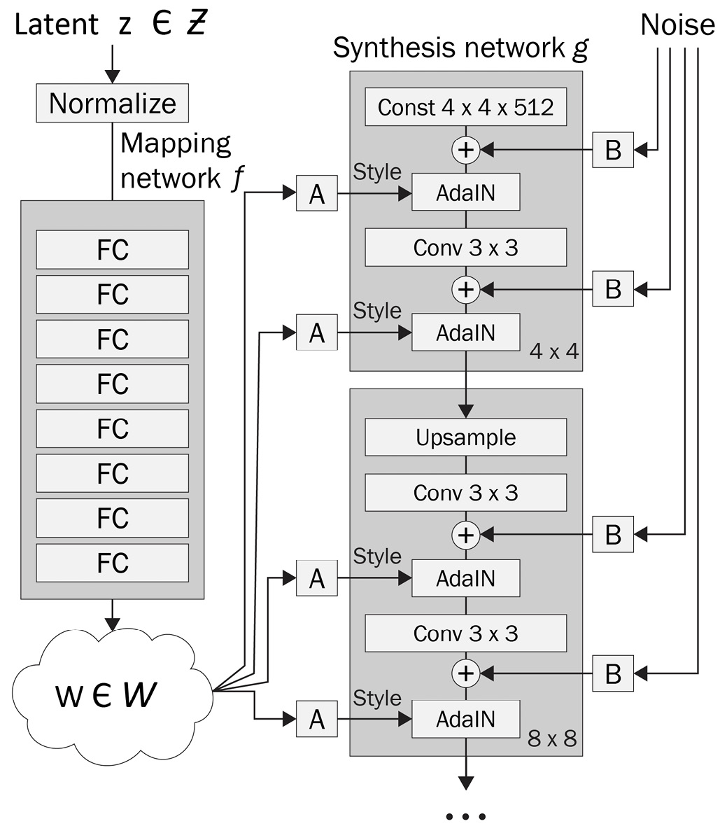
Figure 3.5 – A mapping network (left) and generator (right) of StyleGAN

In the preceding figure, the network that takes in a latent vector, z, and generates w is the mapping network. The network on the right is the generator, g, which takes in a set of noise vectors, as well as w. The discriminator is fairly simple compared to the generator. The layers are depicted in Figure 3.6:

Figure 3.6 – A StyleGAN discriminator architecture for the FFHQ dataset at 1024 × 1024 resolution

As depicted in the preceding image, the discriminator consists of multiple blocks of convolution layers and downsampling operations. It takes in an image of size 1024 x 1024 and generates a numeric value between 0 and 1, describing how realistic the image is.

Training StyleGAN

Training StyleGAN requires a lot of computations, so multiple GPUs are necessary to achieve a reasonable training time. The estimations are summarized in Figure 3.7:

Figure 3.7 – The training time for StyleGAN with an FFHQ dataset on Tesla V100 GPUs

Therefore, if you want to play around with StyleGAN, we recommend following the instructions in the official GitHub repositories, where they provide pre-trained models: https://github.com/NVlabs/stylegan.

Implementation in PyTorch

Unfortunately, NVIDIA has not shared the public implementation of StyleGAN in PyTorch. Instead, they have released StyleGAN2, which shares most of the same components. Therefore, we will use the StyleGAN2 implementation for our PyTorch example: https://github.com/NVlabs/stylegan2-ada-pytorch.

All the network components are found under training/network.py. The three components are named as described in the previous section: MappingNetwork, Generator, and Discriminator.

The mapping network in PyTorch

The implementation of MappingNetwork is self-explanatory. The following code snippet includes the core logic for the mapping network:

class MappingNetwork(torch.nn.Module):
   def __init__(self, ...):
       ...
       for idx in range(num_layers):
          in_features = features_list[idx]
          out_features = features_list[idx + 1]
          layer = FullyConnectedLayer(in_features, out_features, activation=activation, lr_multiplier= lr_multiplier) setattr(self, f'fc{idx}', layer)
       
   def forward(self, z, ...):
       # Embed, normalize, and concat inputs.
       x = normalize_2nd_moment(z.to(torch.float32))
       
       # Main layers
       for idx in range(self.num_layers):
          layer = getattr(self, f'fc{idx}')
          x = layer(x)
       return x

In this network definition, MappingNetwork inherits torch.nn.Module. Within the __init__ function, the necessary FullyConnectedLayer instances are initialized. The forward method feeds the latent vector, z, to each layer.

The generator in PyTorch

The following code snippet describes how the generator is implemented. It consists of MappingNetwork and SynthesisNetwork, as depicted in Figure 3.5:

class Generator(torch.nn.Module):
   def __init__(self, …):
       self.z_dim = z_dim
       self.c_dim = c_dim
       self.w_dim = w_dim
       self.img_resolution = img_resolution
       self.img_channels = img_channels
       self.synthesis = SynthesisNetwork(
          w_dim=w_dim, 
          img_resolution=img_resolution,
          img_channels=img_channels,
          synthesis_kwargs)
       self.num_ws = self.synthesis.num_ws
       self.mapping = MappingNetwork(
          z_dim=z_dim, c_dim=c_dim, w_dim=w_dim,
          num_ws=self.num_ws, **mapping_kwargs)
   def forward(self, z, c, truncation_psi=1, truncation_cutoff=None, **synthesis_kwargs):
       ws = self.mapping(z, c, 
       truncation_psi=truncation_psi, 
       truncation_cutoff=truncation_cutoff)
       img = self.synthesis(ws, **synthesis_kwargs)
       return img

The generator network, Generator, also inherits torch.nn.Module. SynthesisNetwork and MappingNetwork are instantiated within the __init__ function and get triggered sequentially in the forward function. The implementation of SynthesisNetwork is summarized in the following code snippet:

class SynthesisNetwork(torch.nn.Module):
   def __init__(self, ...):
       for res in self.block_resolutions:
          block = SynthesisBlock(
             in_channels, out_channels, w_dim=w_dim,
             resolution=res, img_channels=img_channels,
             is_last=is_last, use_fp16=use_fp16,
             block_kwargs)
          setattr(self, f'b{res}', block)
       ...
   def forward(self, ws, **block_kwargs):
       ...
       x = img = None
       for res, cur_ws in zip(self.block_resolutions, block_ws):
          block = getattr(self, f'b{res}')
          x, img = block(x, img, cur_ws, **block_kwargs)
       return img

SynthesisNetwork has multiple blocks of SynthesisBlock. SynthesisBlock receives noise vectors and the output of MappingNetwork to generate a tensor that eventually becomes the output image.

The discriminator in PyTorch

The following code snippet summarizes the PyTorch implementation of Discriminator. The network architecture follows the structure depicted in Figure 3.6:

class Discriminator(torch.nn.Module):
   def __init__(self, ...):
       self.block_resolutions = [2 ** i for i in range(self.img_resolution_log2, 2, -1)]
       for res in self.block_resolutions:
          block = DiscriminatorBlock(
              in_channels, tmp_channels, out_channels,
              resolution=res,
              first_layer_idx = cur_layer_idx,
              use_fp16=use_fp16, **block_kwargs, 
              common_kwargs)
          setattr(self, f'b{res}', block)
   def forward(self, img, c, **block_kwargs):
       x = None
       for res in self.block_resolutions:
          block = getattr(self, f'b{res}')
          x, img = block(x, img, **block_kwargs)
       return x

Similar to SynthesisNetwork, Discriminator makes use of the DiscriminatorBlock class to dynamically create a set of convolutional layers of different sizes. They are defined in the __init__ function, and the tensors are fed to each block sequentially in the forward function.

Model training logic in PyTorch

Training logic is defined in the training_loop function in training/train_loop.py. The original implementation contains a lot of details. In the following code snippet, we will look at the main components that align with what we have learned in the PyTorch model training section:

def training_loop(...):
   ...
training_set_iterator = iter(torch.utils.data.DataLoader(dataset=training_set, sampler=training_set_sampler, batch_size=batch_size//num_gpus, **data_loader_kwargs))
   loss = dnnlib.util.construct_class_by_name(device=device, **ddp_modules, **loss_kwargs) # subclass of training.loss.Loss
   while True:
      # Fetch training data.
      with torch.autograd.profiler.record_function('data_fetch'):
         phase_real_img, phase_real_c = next(training_set_iterator)
      # Execute training phases.
      for phase, phase_gen_z, phase_gen_c in zip(phases, all_gen_z, all_gen_c):
         # Accumulate gradients over multiple rounds.
      for round_idx, (real_img, real_c, gen_z, gen_c) in enumerate(zip(phase_real_img, phase_real_c, phase_gen_z, phase_gen_c)):
         loss.accumulate_gradients(phase=phase.name, real_img=real_img, real_c=real_c, gen_z=gen_z, gen_c=gen_c, sync=sync, gain=gain)
      # Update weights.
      phase.module.requires_grad_(False)
      with torch.autograd.profiler.record_function(phase.name + '_opt'):
         phase.opt.step()

This function receives configurations for various training components and trains both Generator and Discriminator. The outer loop iterates over training samples, and the inner loop handles gradient calculation and model parameter updates. The training settings are configured by a separate script, main/train.py.

This summarizes the structure of PyTorch implementation. Even though the repository looks overwhelming due to the large number of files, we have walked you through how to break the implementation down into the components that we have described in the Implementing and training a model in PyTorch section. In the following section, we will look at implementation in TF.

Implementation in TF

Even though the official implementation is in TF (https://github.com/NVlabs/stylegan), we will look at a different implementation presented in Hands-On Image Generation with TensorFlow: A Practical Guide to Generating Images and Videos Using Deep Learning by Soon Yau Cheong. This version is based on TF version 2 and aligns better with what we have described in this book. The implementation can be found at https://github.com/PacktPublishing/Hands-On-Image-Generation-with-TensorFlow-2.0/blob/master/Chapter07/ch7_faster_stylegan.ipynb.

Similar to the PyTorch implementation described in the previous section, the original TF implementation consists of G_mapping for the mapping network, G_style for the generator, and D_basic for the discriminator.

The mapping network in TF

Let’s look at the mapping network defined at https://github.com/NVlabs/stylegan/blob/1e0d5c781384ef12b50ef20a62fee5d78b38e88f/training/networks_stylegan.py#L384 and its TF version 2 implementation shown below:

def Mapping(num_stages, input_shape=512):
   z = Input(shape=(input_shape))
   w = PixelNorm()(z)
   for i in range(8):
      w = DenseBlock(512, lrmul=0.01)(w)
      w = LeakyReLU(0.2)(w)
      w = tf.tile(tf.expand_dims(w, 1), (1,num_stages,1))
   return Model(z, w, name='mapping') 

The implementation of MappingNetwork is almost self-explanatory. We can see that the mapping network starts with vector w constructed from a latent vector, z, using a PixelNorm custom layer. The custom layer is defined as follows:

class PixelNorm(Layer):
   def __init__(self, epsilon=1e-8):
      super(PixelNorm, self).__init__()
      self.epsilon = epsilon                
   def call(self, input_tensor):
      return input_tensor / tf.math.sqrt(tf.reduce_mean(input_tensor**2, axis=-1, keepdims=True) + self.epsilon)

As described in the TF dense (linear) layers section, PixelNorm inherits the tensorflow.keras.layers.Layer class and defines the computation within the call function.

The remaining components of Mapping are a set of dense layers with LeakyReLU activations.

Next, we will have a look at the generator network.

The generator in TF

The generator in the original code, G_style, is composed of two networks: G_mapping and G_synthesis. See the following: https://github.com/NVlabs/stylegan/blob/1e0d5c781384ef12b50ef20a62fee5d78b38e88f/training/networks_stylegan.py#L299.

The complete implementation from the repository might look extremely complex at first. However, you will soon find out that G_style simply calls G_mapping and G_synthesis sequentially.

The implementation of SynthesisNetwork is summarized in the following code snippet: https://github.com/NVlabs/stylegan/blob/1e0d5c781384ef12b50ef20a62fee5d78b38e88f/training/networks_stylegan.py#L440.

In TF version 2, the generator is implemented as follows:

def GenBlock(filter_num, res, input_shape, is_base):
   input_tensor = Input(shape=input_shape, name=f'g_{res}')
   noise = Input(shape=(res, res, 1), name=f'noise_{res}')
   w = Input(shape=512)
   x = input_tensor
   if not is_base:
      x = UpSampling2D((2,2))(x)
      x = ConvBlock(filter_num, 3)(x)
   x = AddNoise()([x, noise])
   x = LeakyReLU(0.2)(x)
   x = InstanceNormalization()(x)
   x = AdaIN()([x, w])
   # Adding noise
   x = ConvBlock(filter_num, 3)(x)
   x = AddNoise()([x, noise])
   x = LeakyReLU(0.2)(x)
   x = InstanceNormalization()(x)                    
   x = AdaIN()([x, w])
   return Model([input_tensor, w, noise], x, name=f'genblock_{res}x{res}')

This network follows the architecture depicted in Figure 3.5; SynthesisNetwork is constructed with a set of AdaIn and ConvBlock custom layers.

Let’s move on to the discriminator network.

The discriminator in TF

The D_basic function implements the discriminator depicted in Figure 3.6. (https://github.com/NVlabs/stylegan/blob/1e0d5c781384ef12b50ef20a62fee5d78b38e88f/training/networks_stylegan.py#L562). Since the discriminator consists of a set of convolution layer blocks, D_basic has a dedicated function, block, that builds a block based on the input tensor size. The core components of the function look as follows:

def block(x, res): # res = 2 … resolution_log2
   with tf.variable_scope('%dx%d' % (2**res, 2**res)):
       x = act(apply_bias(conv2d(x, fmaps=nf(res-1), kernel=3, gain=gain, use_wscale=use_wscale)))
       x = act(apply_bias(conv2d_downscale2d(blur(x), fmaps=nf(res-2), kernel=3, gain=gain, use_wscale=use_wscale, fused_scale=fused_scale)))
   return x

In the preceding code, the block function deals with creating each block in the discriminator by combining convolution and downsampling layers. The remaining logic of D_basic is straightforward, as it simply chains a set of convolution layer blocks by passing the output of one block as an input to the next block.

Model training logic in TF

The training logic for TF implementation can be found in the train_step function. Understanding the implementation details should not be challenging as they have followed the description we had in the TF model training section.

Overall, we have learned how StyleGAN can be implemented in TF version 2 using the TF building blocks that we described in this chapter.

Things to remember

a. Any DL model training implementation can be broken into three components (data loading logic, model definition, and model training logic), regardless of the complexity of the implementation.

At this stage, you should understand how the StyleGAN repository is structured in each framework. We strongly recommend that you play around with the pre-trained models to generate interesting images. If you master StyleGAN, it should be easy to follow the implementation of StyleGAN2 (https://arxiv.org/abs/1912.04958), StyleGAN3 (https://arxiv.org/abs/2106.12423), and HyperStyle (https://arxiv.org/abs/2111.15666).

Summary

In this chapter, we have explored where the flexibility of DL comes from. DL uses a network of mathematical neurons to learn the hidden patterns within a set of data. Training a network involves the iterative process of updating model parameters based on a train set and selecting the model that performs the best on a validation set, with the goal of producing the best performance on a test set.

Realizing the repeated processes within model training, many engineers and researchers have put together common building blocks into frameworks. We have described two of the most popular frameworks: PyTorch and TF. The two frameworks are structured in a similar way, allowing users to set up the model training using three building blocks: data loading logic, model definition, and model training logic. As the final topic of the chapter, we decomposed StyleGAN, one of the most popular GAN implementations, to understand how the building blocks are used in reality.

As DL requires a large amount of data for successful training, efficient management of the data, model implementations, and various training results are critical to the success of any project. In the following chapter, we will introduce useful tools for DL experiment monitoring.