
Chapter 12
Application Case Study
Molecular Visualization and Analysis
Chapter Outline
12.1 Application Background
12.2 A Simple Kernel Implementation
12.3 Thread Granularity Adjustment
12.4 Memory Coalescing
12.5 Summary
12.6 Exercises
The previous case study illustrated the process of selecting an appropriate level of a loop nest for parallel execution, the use of constant memory for magnifying the memory bandwidth for read-only data, the use of registers to reduce the consumption of memory bandwidth, and the use of special hardware functional units to accelerate trigonometry functions. In this case study, we use an application based on regular grid data structures to illustrate the use of additional practical techniques that achieve global memory access coalescing and improved computation throughput. We present a series of implementations of an electrostatic potential map calculation kernel, with each version improving upon the previous one. Each version adopts one or more practical techniques. This computation pattern of this application is one of the best matches for massively parallel computing. This application case study shows that the effective use of these practical techniques can significantly improve the execution throughput and is critical for the application to achieve its potential performance.
12.1 Application Background
This case study is based on VMD (Visual Molecular Dynamics) [HDS1996], a popular software system designed for displaying, animating, and analyzing biomolecular systems. As of 2012, VMD has more than 200,000 registered users. While it has strong built-in support for analyzing biomolecular systems, such as calculating electrostatic potential values at spatial grid points of a molecular system, it has also been a popular tool for displaying other large data sets, such as sequencing data, quantum chemistry simulation data, and volumetric data, due to its versatility and user extensibility.
While VMD is designed to run on a diverse range of hardware—laptops, desktops, clusters, and supercomputers—most users use VMD as a desktop science application for interactive 3D visualization and analysis. For computation that runs too long for interactive use, VMD can also be used in a batch mode to render movies for later use. A motivation for accelerating VMD is to make batch mode jobs fast enough for interactive use. This can drastically improve the productivity of scientific investigations. With CUDA devices widely available in desktop PCs, such acceleration can have broad impact on the VMD user community. To date, multiple aspects of VMD have been accelerated with CUDA, including electrostatic potential calculation, ion placement, molecular orbital calculation and display, and imaging of gas migration pathways in proteins.
The particular calculation used in this case study is the calculation of electrostatic potential maps in a grid space. This calculation is often used in placement of ions into a structure for molecular dynamics simulation. Figure 12.1 shows the placement of ions into a protein structure in preparation for molecular dynamics simulation. In this application, the electrostatic potential map is used to identify spatial locations where ions (round dots around the large molecules) can fit in according to physical laws. The function can also be used to calculate time-averaged potentials during molecular dynamics simulation, which is useful for the simulation process as well as the visualization/analysis of simulation results.
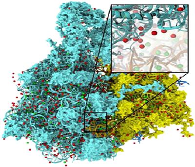
Figure 12.1 Electrostatic potential map is used in building stable structures for molecular dynamics simulation.
There are several methods for calculating electrostatic potential maps. Among them, direct coulomb summation (DCS) is a highly accurate method that is particularly suitable for GPUs [SPF2007]. The DCS method calculates the electrostatic potential value of each grid point as the sum of contributions from all atoms in the system. This is illustrated in Figure 12.2. The contribution of atom i to a lattice point j is the charge of that atom divided by the distance from lattice point j to atom i. Since this needs to be done for all grid points and all atoms, the number of calculations is proportional to the product of the total number of atoms in the system and the total number of grid points. For a realistic molecular system, this product can be very large. Therefore, the calculation of the electrostatic potential map has been traditionally done as a batch job in VMD.
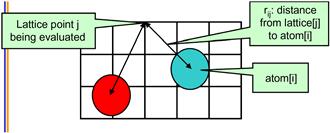
Figure 12.2 The contribution of atom[i] to the electrostatic potential at lattice point j (potential[j]) is atom[i].charge/rij. In the DCS method, the total potential at lattice point j is the sum of contributions from all atoms in the system.
12.2 A Simple Kernel Implementation
Figure 12.3 shows the base C code of the DCS code. The function is written to process a 2D slice of a 3D grid. The function will be called repeatedly for all the slices of the modeled space. The structure of the function is quite simple with three levels of for loops. The outer two levels iterate over the y dimension and the x dimension of the grid point space. For each grid point, the innermost for loop iterates over all atoms, calculating the contribution of electrostatic potential energy from all atoms to the grid point. Note that each atom is represented by four consecutive elements of the atoms[] array. The first three elements store the x, y, and z coordinates of the atom and the fourth element the electrical charge of the atom. At the end of the innermost loop, the accumulated value of the grid point is written out to the grid data structure. The outer loops then iterate and take the execution to the next grid point.
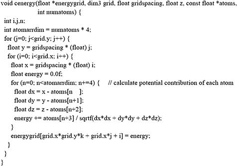
Figure 12.3 Base coulomb potential calculation code for a 2D slice.
Note that the DCS function in Figure 12.3 calculates the x and y coordinates of each grid point on-the-fly by multiplying the grid point index values by the spacing between grid points. This is a uniform grid method where all grid points are spaced at the same distance in all three dimensions. The function does take advantage of the fact that all the grid points in the same slice have the same z coordinate. This value is precalculated by the caller of the function and passed in as a function parameter (z).
Based on what we learned from the MRI case study, two attributes of the DCS method should be apparent. First, the computation is massively parallel: the computation of electrostatic potential for each grid point is independent of that of other grid points. There are two alternative approaches to organizing parallel execution. In the first option, we can use each thread to calculate the contribution of one atom to all grid points. This would be a poor choice since each thread would be writing to all grid points, requiring extensive use of atomic memory operations to coordinate the updates done by different threads to each grid point. The second option uses each thread to calculate the accumulated contributions of all atoms to one grid point. This is a preferred approach since each thread will be writing into its own grid point and there is no need to use atomic operations.
We will form a 2D thread grid that matches the 2D energy grid point organization. To do so, we need to modify the two outer loops into perfectly nested loops so that we can use each thread to execute one iteration of the two-level loop. We can either perform a loop fission, or we move the calculation of the y coordinate into the inner loop. The former would require us to create a new array to hold all y values and result in two kernels communicating data through global memory. The latter increases the number of times that the y coordinate will be calculated. In this case, we choose to perform the latter since there is only a small amount of calculation that can be easily accommodated into the inner loop without a significant increase in execution time of the inner loop. The former would have added a kernel launch overhead for a kernel where threads do very little work. The selected transformation allows all i and j iterations to be executed in parallel. This is a trade-off between the amount of calculation done and the level of parallelism achieved.
The second experience that we can apply from the MRI case study is that the electrical charge of every atom will be read by all threads. This is because every atom contributes to every grid point in the DCS method. Furthermore, the values of the atomic electrical charges are not modified during the computation. This means that the atomic charge values can be efficiently stored in the constant memory (in the GPU box in Figure 12.4).
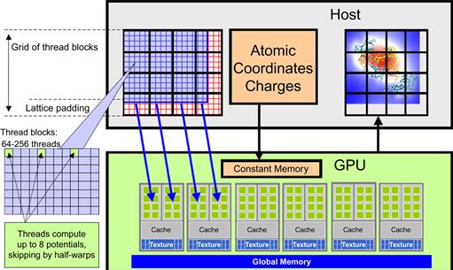
Figure 12.4 Overview of the DCS kernel design.
Figure 12.4 shows an overview of the DCS kernel design. The host program (host box in Figure 12.4) inputs and maintains the atomic charges and their coordinates in the system memory. It also maintains the grid point data structure in the system memory (left side in the host box). The DCS kernel is designed to process a 2D slice of the energy grid point structure (not to be confused with thread grids). The right side grid in the host box shows an example of a 2D slice. For each 2D slice, the CPU transfers its grid data to the device global memory. The atom information is divided into chunks to fit into the constant memory. For each chunk of the atom information, the CPU transfers the chunk into the device constant memory, invokes the DCS kernel to calculate the contribution of the current chunk to the current slice, and prepares to transfer the next chunk. After all chunks of the atom information have been processed for the current slice, the slice is transferred back to update the grid point data structure in the CPU system memory. The system moves on to the next slice.
Within each kernel invocation, the thread blocks are organized to calculate the electrostatic potential of tiles of the grid structure. In the simplest kernel, each thread calculates the value at one grid point. In more sophisticated kernels, each thread calculates multiple grid points and exploits the redundancy between the calculations of the grid points to improve execution speed. This is illustrated in the left side portion labeled as “thread blocks” in Figure 12.4 and is an example of the granularity adjustment optimization discussed in Chapter 6.
Figure 12.5 shows the resulting CUDA kernel code. We omitted some of the declarations. As was the case in the MRI case study, the atominfo[] array is declared in the constant memory by the host code. The host code also needs to divide up the atom information into chunks that fit into the constant memory for each kernel invocation. This means that the kernel will be invoked multiple times when there are multiple chunks of atoms. Since this is similar to the MRI case study, we will not show the details.

Figure 12.5 DCS kernel version 1.
The outer two levels of the loop in Figure 12.3 have been removed from the kernel code and are replaced by the execution configuration parameters in the kernel invocation. Since this is also similar to one of the steps we took in the MRI case study, we will not show the kernel invocation but leave it as an exercise for readers. The rest of the kernel code is straightforward and corresponds directly to the original loop body of the innermost loop.
One particular aspect of the kernel is somewhat subtle and worth mentioning. The kernel code calculates the contribution of a chunk of atoms to a grid point. The grid point must be preserved in the global memory and updated by each kernel invocation. This means that the kernel needs to read the current grid point value, add the contributions by the current chunk of atoms, and write the updated value to global memory. The code attempts to hide the global memory latency by loading the grid value at the beginning of the kernel and using it at the end of the kernel. This helps to reduce the number of warps needed by the streaming multiprocessor (SM) scheduler to hide the global memory latency.
The performance of the kernel in Figure 12.5 is quite good, measured at 186 GFLOPS on a G80, a first-generation CUDA device. In terms of application-level performance, the implementation can process 18.6 billion atom evaluations per second. A quick glance over the code shows that each thread does nine floating-point operations for every four memory elements accessed. On the surface, this is not a very good ratio. We need at least a ratio of 8 to avoid global memory congestion. However, all four memory accesses are done to the atominfo[] array. These atominfo[] array elements for each atom are cached in a hardware cache memory in each SM and are broadcast to a large number of threads. A similar calculation to that in the MRI case study shows that the massive reuse of memory elements across threads make the constant cache extremely effective, boosting the effective ratio of floating operations per global memory access much higher than 10:1. As a result, global memory bandwidth is not a limiting factor for this kernel.
12.3 Thread Granularity Adjustment
Although the kernel in Figure 12.5 avoids global memory bottleneck through constant caching, it still needs to execute four constant memory access instructions for every nine floating-point operations performed. These memory access instructions consume hardware resources that could be otherwise used to increase the execution throughput of floating-point instructions. This section shows that we can fuse several threads together so that the atominfo[] data can be fetched once from the constant memory, stored into registers, and used for multiple grid points. This idea is illustrated in Figure 12.6.
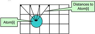
Figure 12.6 Reusing information among multiple grid points.
Furthermore, all grid points along the same row have the same y coordinate. Therefore, the difference between the y coordinate of an atom and the y coordinate of any grid point along a row has the same value. In the DCS kernel version 1 in Figure 12.5, this calculation is redundantly done by all threads for all grid points in a row when calculating the distance between the atom and the grid points. We can eliminate this redundancy and improve the execution efficiency.
The idea is to have each thread to calculate the electrostatic potential for multiple grid points. The kernel in Figure 12.7 has each thread calculate four grid points. For each atom, the code calculates dy, the difference of the y coordinate in line 2. It then calculates the expression dy∗dy plus the precalculated dz∗dz information and saves it to the auto variable dysqpdzsq, which is assigned to a register by default. This value is the same for all four grid points. Therefore, the calculation of energyvalx1 through energyvalx4 can all just use the value stored in the register. Furthermore, the electrical charge information is also accessed from constant memory and stored in the automatic variable charge. Similarly, the x coordinate of the atom is also read from constant memory into auto variable x. Altogether, this kernel eliminates three accesses to constant memory for atominfo[atomid].y, three accesses to constant memory for atominfo[atomid].x, three accesses to constant memory for atominfo[atomid].w, three floating-point subtraction operations, five floating-point multiply operations, and nine floating-point add operations when processing an atom for four grid points. A quick inspection of the kernel code in Figure 12.7 shows that each iteration of the loop performs four constant memory accesses, five floating-point subtractions, nine floating-point additions, and five floating-point multiplications for four grid points.
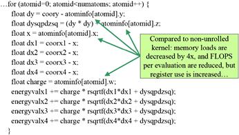
Figure 12.7 DCS kernel version 2.
Readers should also verify that the version of DCS kernel in Figure 12.5 performs 16 constant memory accesses, 8 floating-point subtractions, 12 floating-point additions, and 12 floating-point multiplications, for a total of 48 operations for the same four grid points. Going from Figure 12.5 to Figure 12.7, there is a total reduction from 48 operations down to 25 operations, a sizable reduction. This is translated into an increased execution speed from 186 GFLOPS to 259 GFLOPS on a G80. In terms of application-level throughput, the performance increases from 18.6 billion atom evaluations per second to 33.4 billion atom evaluations per second. The reason that the application-level performance improvement is higher than the FLOPS improvement is that some of the floating-point operations have been eliminated.
The cost of the optimization is that more registers are used by each thread. This reduces the number of threads that can be assigned to each SM. However, as the results show, this is a good trade-off with an excellent performance improvement.
12.4 Memory Coalescing
While the performance of the DCS kernel version 2 in Figure 12.7 is quite high, a quick profiling run reveals that the threads perform memory writes inefficiently. As shown in Figures 12.6 and 12.7, each thread calculates four neighboring grid points. This seems to be a reasonable choice. However, as we illustrate in Figure 12.8, the access pattern of threads will result in uncoalesced global memory writes.
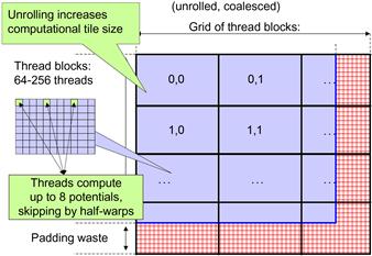
Figure 12.8 Organizing threads and memory layout for coalesced writes.
There are two problems that cause the uncoalesced writes in DCS kernel version 2. First, each thread calculates four adjacent neighboring grid points. Thus, for each statement that accesses the energygrid[] array, the threads in a warp are not accessing adjacent locations. Note that two adjacent threads access memory locations that are three elements apart. Thus, the 16 locations to be written by all the threads in warp write are spread out, with three elements in between the loaded/written locations. This problem can be solved by assigning adjacent grid points to adjacent threads in each half-warp. Assuming that we still want to have each thread calculate four grid points, we first assign 16 consecutive grid points to the 16 threads in a half-warp. We then assign the next 16 consecutive grid points to the same 16 threads. We repeat the assignment until each thread has the number of grid points desired. This assignment is illustrated in Figure 12.8. With some experimentation, the best number of grid points per thread turns out to be 8 for G80.
The kernel code with a warp-aware assignment of grid points to threads is shown in Figure 12.9. Note that the x coordinates used to calculate the distances are offset by the variable gridspacing_coalescing, which is the original grid spacing times the constant BLOCKSIZE (16). This reflects the fact that the x coordinates of the 8 grid points are 16 grid points away from each other. Also, after the end of the loop, memory writes to the energygrid[] array are indexed by outaddr, outaddr+BLOCKSIZE, …, outaddr+7∗BLOCKSIZE. Each of these indices is one BLOCKSIZE (16) away from the previous one. The detailed thread block organization for this kernel is left as an exercise. Readers should keep in mind that by setting the x dimension size of the thread block to be equal to the half-warp size (16), we can simplify the indexing in the kernel.
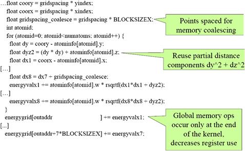
Figure 12.9 DCS kernel version 3.
The other cause of uncoalesced memory writes is the layout of the energygrid[] array, which is a 3D array. If the x dimension of the array is not a multiple of half-warp size, the beginning location of the second row, as well as those of the subsequent rows, will no longer be at the 16-word boundaries. In older devices, this means that the half-warp accesses will not be coalesced, even though they write to consecutive locations. This problem can be corrected by padding each row with additional elements so that the total length of the x dimension is a multiple of 16. This can require adding up to 15 elements, or 60 bytes to each row, as shown in Figure 12.8. With the kernel of Figure 12.9, the number of elements in the x dimension needs to be a multiple of 8×16=128. This is because each thread actually writes 8 elements in each iteration. Thus, one may need to pad up to 127 elements, or 1,016 bytes, to each row.
Furthermore, there is a potential problem with the last row of thread blocks. Since the grid array may not have enough rows, some of the threads may end up writing outside the grid data structure. Since the grid data structure is a 3D array, these threads will write into the next slice of grid points. As we discussed in Chapter 3, we can add a test in the kernel and avoid writing the array elements that are out of the known y dimension size. However, this would have added a number of overhead instructions and incurred control divergence. Another solution is to pad the y dimension of the grid structure so that it contains a multiple of tiles covered by thread blocks. This is shown in Figure 12.8 as the bottom padding in the grid structure. In general, one may need to add up to 15 rows due to this padding.
The cost of padding can be substantial for smaller grid structures. For example, if the energy grid has 100×100 grid points in each 2D slice, it would be padded into a 128×112 slice. The total number of grid points increase from 10,000 to 14,336, or a 43% overhead. If we had to pad the entire 3D structure, the grid points would have increased from 100×100×100 (1,000,000) to 128×112×112 (1,605,632), or a 60% overhead! This is part of the reason why we calculate the energy grids in 2D slices and use the host code to iterate over these 2D slices. Writing a single kernel to process the entire 3D structure would have incurred a lot more extra overhead. This type of trade-off appears frequently in simulation models, differential equation solvers, and video processing applications.
The DCS version 3 kernel shown in Figure 12.9 achieves about 291 GFLOPs, or 39.5 billion atom evaluations per second on a G80. On a later Fermi device, it achieves 535.16 GFLOPS, or 72.56 billion atom evaluations per sec. On a recent GeForce GTX680 Kepler 1, it achieves a whopping 1267.26 GFLOPS, or 171.83 billion atom evaluations per sec! This measured speed of the kernel also includes a slight boost from moving the read access to the energygrid[] array from the beginning of the kernel to the end of the kernel. The contribution to the grid points are first calculated in the loop. The code loads the original grid point data after the loop, adds the contribution to the data, and writes the updated values back. Although this movement exposes more of the global memory latency to each thread, it saves the consumption of eight registers. Since the kernel is already using many registers to hold the atom data and the distances, such savings in number of registers used relieves a critical bottleneck for the kernel. This allows more thread blocks to be assigned to each SM and achieves an overall performance improvement.
12.5 Summary
Figure 12.10 shows a summary of the performance comparison between the various DCS kernel implementations and how they compare with an optimized single-core CPU execution. One important observation is that the relative merit of the kernels varies with grid dimension lengths. However, the DCS version 3 (CUDA-Unroll8clx) performs consistently better than all others once the grid dimension length is larger than 300.
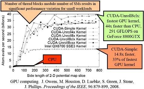
Figure 12.10 Performance comparison of various DCS kernel versions.
A detailed comparison between the CPU performance and the CPU–GPU joint performance shows a commonly observed trade-off. Figure 12.11 shows plot of the execution time of a medium-size grid system for a varying number of atoms to be evaluated. For 400 atoms or fewer, the CPU performs better. This is because the GPU has a fixed initialization overhead of 110 ms regardless of the number of atoms to be evaluated. Also, for a small number of atoms, the GPU is underutilized, thus the curve of the GPU execution time is quite flat between 100 and 1,000 atoms.
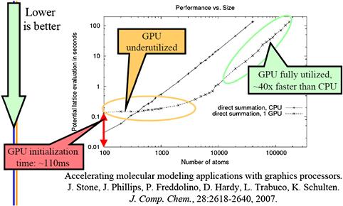
Figure 12.11 Single-thread CPU versus CPU–GPU comparison.
The plot in Figure 12.11 reenforces a commonly held principle that GPUs perform better for large amounts of data. Once the number of atoms reaches 10,000, the GPU is fully utilized. The slopes of the CPU and the CPU–GPU execution time become virtually identical, with the CPU–GPU execution being consistently 44× times faster than the CPU execution for all input sizes.
12.6 Exercises
12.1. Complete the implementation of the DCS kernel as outlined in Figure 12.5. Fill in all the missing declarations. Give the kernel launch statement with all the execution configuration parameters.
12.2. Compare the number of operations (memory loads, floating-point arithmetic, branches) executed in each iteration of the kernel in Figure 12.7 compared to that in Figure 12.5. Keep in mind that each iteration of the former corresponds to four iterations of the latter.
12.3. Complete the implementation of the DCS kernel version 3 in Figure 12.9. Explain in your own words how the thread accesses are coalesced in this implementation.
12.4. For the memory padding in Figure 12.8 and DCS kernel version 3 in Figure 12.9, show why one needs to pad up to 127 elements in the x dimension but only up to 15 elements in the y dimension.
12.5. Give two reasons for adding extra “padding” elements to arrays allocated in the GPU global memory, as shown in Figure 12.8.
12.6. Give two potential disadvantages associated with increasing the amount of work done in each CUDA thread, as shown in Section 12.3.
References
1. Humphrey W, Dalke A, Schulten K. VMD—Visual Molecular Dynamics. Journal of Molecular Graphics. 1996;14:33–38.
2. Stone JE, Phillips JC, Freddolino PL, Hardy DJ, Trabuco LG, Schulten K. Accelerating molecular modeling applications with graphics processors. Journal of Computational Chemistry. 2007;28:2618–2640.