
Chapter 15
Parallel Programming with OpenACC
Chapter Outline
15.1 OpenACC Versus CUDA C
15.2 Execution Model
15.3 Memory Model
15.4 Basic OpenACC Programs
15.5 Future Directions of OpenACC
15.6 Exercises
The OpenACC Application Programming Interface (API) provides a set of compiler directives, library routines, and environment variables that can be used to write data-parallel FORTRAN, C, and C++ programs that run on accelerator devices, including GPUs. It is an extension to the host language. The OpenACC specification was initially developed by the Portland Group (PGI), Cray Inc., and NVIDIA, with support from CAPS enterprise. This chapter presents an introduction to OpenACC to parallel programmers who are already familiar with CUDA C.
15.1 OpenACC Versus CUDA C
One big difference between OpenACC and CUDA C is the use of compiler directives in OpenACC. To understand what a compiler directive is and the advantages of using compiler directives, let’s take a look at our first OpenACC program in Figure 15.1, which does the matrix multiplication that we’ve already seen before.
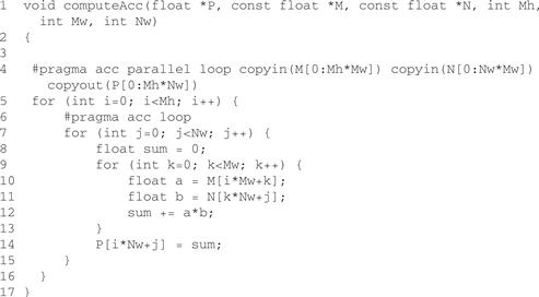
Figure 15.1 Our first OpenACC program.
The code in the figure is almost identical to the sequential version, except for the two lines with #pragma at lines 4 and 6. In C and C++, the #pragma directive is the method to provide, to the compiler, information that is not specified in the standard language. OpenACC uses the compiler directive mechanism to extend the base language. In this example, the #pragma at line 4 tells the compiler to generate code for the i loop at lines 5-16 so that the loop iterations are executed in parallel on the accelerator. The copyin clause and the copyout clause specify how the matrix data should be transferred between the host and the accelerator. The #pragma at line 6 instructs the compiler to map the inner j loop to the second level of parallelism on the accelerator.
Compared with CUDA C/C++/FORTRAN, by using compiler directives, OpenACC brings quite a few benefits to programmers:
• OpenACC programmers can often start with writing a sequential version and then annotate their sequential program with OpenACC directives. They can leave most of the heavy lifting to the OpenACC compiler. The details of data transfer between host and accelerator memories, data caching, kernel launching, thread scheduling, and parallelism mapping are all handled by OpenACC compiler and runtime. The entry barrier of heterogeneous programmers for accelerators becomes much lower with OpenACC.
• OpenACC provides an incremental path for moving legacy applications to accelerators. This is attractive because adding directives disturbs the existing code less than other approaches. Some existing scientific applications are large and their developers don’t want to rewrite them for accelerators. OpenACC lets these developers keep their applications looking like normal C, C++, or FORTRAN code, and they can go in and put the directives in the code where they are needed one place a time.
• A non-OpenACC compiler is not required to understand and process OpenACC directives, therefore it can just ignore the directives and compile the rest of the program as usual. By using the compiler directive approach, OpenACC allows a programmer to write OpenACC programs in such a way that when the directives are ignored, the program can still run sequentially and gives the same result as when the program is run in parallel. Parallel programs that have equivalent sequential versions are much easier to debug than those that don’t have. The matrix multiplication code in Figure 15.1 has this property—the code gives the same result regardless of whether lines 4 and 6 are honored or not. Such programs essentially have both the parallel version and the sequential version in one. OpenACC permits a common code base for accelerated and nonaccelerated enabled systems.
OpenACC users need to be aware of the following issues:
• Some OpenACC directives are hints to the OpenACC compiler, which may or may not be able to take full advantage of such hints. Therefore, the performance of an OpenACC program depends more on the capability of the OpenACC compiler used. On the other hand, a CUDA C/C++/FORTRAN program expresses parallelism explicitly and relies less on the compiler for parallel performance.
• While it is possible to write OpenACC programs that give the same execution result as when the directives are ignored, this property does not hold automatically for all OpenACC programs. If compiler directives are ignored, some OpenACC programs may give different results or some may not work correctly.
In the rest of this chapter, we first explain the execution model and memory model used by OpenACC. We then walk through some concrete code examples to illustrate usage of some of the more commonly used OpenACC directives and APIs. We also show how an OpenACC implementation can map parallel regions and kernel regions to the CUDA GPU architecture. We believe certain behind-the-scenes knowledge can help users to get the better performance out of OpenACC implementations. We conclude this article by outlining the future directions we see OpenACC going in.
15.2 Execution Model
The OpenACC target machine has a host and an attached accelerator device, such as a GPU. Most accelerator devices can support multiple levels of parallelism. Figure 15.2 illustrates a typical accelerator that supports three levels of parallelism. At the outermost coarse-grain level, there are multiple execution units. Within each execution unit, there are multiple threads. At the innermost level, each thread is capable of executing vector operations. Currently, OpenACC does not assume any synchronization capability on the accelerator, except for thread forking and joining. Once work is distributed among the execution units, they will execute in parallel from start to finish. Similarly, once work is distributed among the threads within an execution unit, the threads execute in parallel. Vector operations are executed in lockstep.

Figure 15.2 A typical accelerator device
An OpenACC program starts its execution on the host single-threaded (Figure 15.3). When the host thread encounters a parallel or a kernels construct, a parallel region or a kernels region that comprises all the code enclosed in the construct is created and launched on the accelerator device. The parallel region or kernels region can optionally execute asynchronously with the host thread and join with the host thread at a future synchronization point. The parallel region is executed entirely on the accelerator device. The kernels region may contain a sequence of kernels, each of which is executed on the accelerator device.
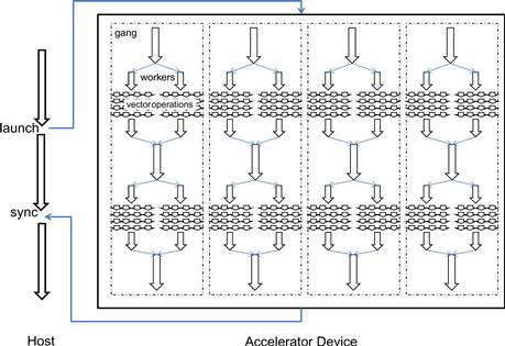
Figure 15.3 OpenACC execution model.
The kernel execution follows a fork-join model. A group of gangs are used to execute each kernel. A group of workers can be forked to execute a parallel work-sharing loop that belongs to a gang. The workers are disbanded when the loop is done. Typically a gang executes on one execution unit, and a worker runs on one thread within an execution unit.
The programmer can instruct how the work within a parallel region or a kernels region is to be distributed among the different levels of parallelism on the accelerator.
15.3 Memory Model
In an OpenACC memory model, the host memory and the device memory are treated as separated. It is assumed that the host is not able to access device memory directly and the device is not able to access host memory directly. This is to ensure that the OpenACC programming model can support a wide range of accelerator devices, including most of the current GPUs that do not have the capability of unified memory access between GPUs and CPUs. The unified virtual addressing and the GPUDirect introduced by NVIDIA in CUDA 4.0 allow a single virtual address space for both host memory and device memory and allow direct cross-device memory access between different GPUs. However, cross-host and device memory access is still not possible.
Just like in CUDA C/C++, in OpenACC input data needs to be transferred from the host to the device before kernel launches and result data needs to be transferred back from the device to the host. However, unlike in CUDA C/C++ where programmers need to explicitly code data movement through API calls, in OpenACC they can just annotate which memory objects need to be transferred, as shown by line 4 in Figure 15.1. The OpenACC compiler will automatically generate code for memory allocation, copying, and de-allocation.
OpenACC adopts a fairly weak consistency model for memory on the accelerator device. Although data on the accelerator can be shared by all execution units, OpenACC does not provide a reliable way to allow one execution unit to consume the data produced by another execution unit. There are two reasons for this. First, recall OpenACC does not provide any mechanism for synchronization between execution units. Second, memories between different execution units are not coherent. Although some hardware provides instructions to explicitly invalidate and update cache, they are not exposed at the OpenACC level. Therefore, in OpenACC, different execution units are expected to work on disjoint memory sets. Threads within an execution unit can also share memory and threads have coherent memory. However, OpenACC currently only mandates a memory fence at the thread fork and join, which are also the only synchronizations OpenACC provides for threads. While the device memory model may appear very limiting, it is not so in practice. For data–race free OpenACC data-parallel applications, the weak memory model works quite well.
15.4 Basic OpenACC Programs
In this section, we will dive in to details of how one can write basic OpenACC programs.
Parallel Construct
Parallel Region, Gangs, and Workers
The single #pragma at line 4 in Figure 15.1 is actually a syntax sugar of two #pragma (Figure 15.4). We explain the parallel construct here and will explain the loop construct in the next section.
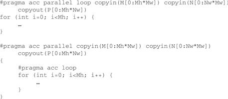
Figure 15.4 #pragma acc parallel loop is #pragma acc parallel and #pragma acc loop in one.
The parallel construct is one of the two constructs (the other is the kernels construct) that can be used to specify which part of the program is to be executed on the accelerator. When a program encounters a parallel construct, the execution of the code within the structured block of the construct (also called a parallel region) is moved to the accelerator. Gangs of workers on the accelerator are created to execute the parallel region, as shown in Figure 15.3. Initially only one worker (let us call it a gang lead) within each gang will execute the parallel region. The other workers are conceptually idle at this point. They will be deployed when there is more parallel work at an inner level. The number of gangs can be specified by the num_gangs clause, and the number of workers within each gang can be specified by the num_workers clause.
In this example (Figure 15.5), a total of 1,024×32=32,768 workers are created. The a=23 statement will be executed in parallel and redundantly by 1,024 gang leads. You may ask why anyone would want to write accelerator code like this. The usefulness of the parallel construct will become clear when it is used with the loop construct.
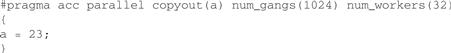
Figure 15.5 Redundant execution in a parallel region.
If a parallel construct does not have an explicit num_gangs clause or an explicit num_workers clause, then the implementation will pick the numbers at runtime. Once a parallel region starts executing, the number of gangs and the number of workers within each gang remain fixed during the execution of the parallel region. This is similar to CUDA in which once a kernel is launched, the number of blocks in the grid and the number of threads in a block cannot be changed.
Loop Construct
Gang Loop
Suppose you have a loop where all the iterations can be independently executed in parallel and you want to speed up its execution by running it on the accelerator. Can you write the code like Figure 15.6?
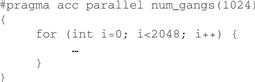
Figure 15.6 An unannotated loop in a parallel region is also redundantly executed.
As we learned from the previous section, although the loop will be executed on the accelerator, you won’t get any speedup because all 2,048 iterations will be executed sequentially and redundantly by the 1,024 gang leads. To get speedup, you need to distribute the 2,048 iterations among the gangs. And to do that, you need to use the gang loop construct, as shown in Figure 15.7.
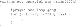
Figure 15.7 Use the loop construct to make a loop work-shared.
A gang loop construct is always associated with a loop. The gang loop construct is a work-sharing construct. The compiler and runtime will make sure that the iterations of a gang loop are shared among all gang leads encountered in the loop construct. In Figure 15.7, because 1,024 gang leads will encounter the loop construct, each lead will be assigned two iterations. Now the execution of the parallel loop will be more efficient and likely to achieve speedup.
Worker Loop
What if you also have an inner loop that can be executed in parallel? Well, that is when the worker loop construct can be beneficial.
The worker loop construct is also a work-sharing construct. The compiler and runtime will make sure that the iterations of a worker loop are shared among all workers within a gang. In Figure 15.8, the 32 workers in a gang will work collectively on the 512 iterations of the j loop in each of the two iterations of the i loop assigned to the gang. A total of 2,048×512=1 M instances of foo() will be executed in the sequential version or the parallel version. In the parallel version, 1,024×32=32 K workers are used and each worker will execute 1 M÷32 K=32 instances of foo().
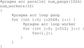
Figure 15.8 Using the worker clause.
OpenACC Versus CUDA
Readers who are familiar with CUDA C may ask how the OpenACC code in Figure 15.8 is different from the CUDA C code in Figure 15.9? They may wonder, can’t I just write the CUDA C version and achieve the same effect?
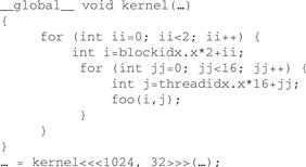
Figure 15.9 A possible CUDA C implementation of the parallel region in Figure 15.8.
Yes, they are similar in this case. And as a matter of fact, some OpenACC implementations may actually generate the CUDA C version in Figure 15.9 from the OpenACC version in Figure 15.8 and pass it to the CUDA C compiler. But one clear advantage of the OpenACC version is that it is much closer to the sequential version than the CUDA C version. Only a few code modifications are required. Compared with CUDA C, OpenACC gives you less control of how the final code on the accelerator will be. However, the strength of OpenACC lies in its ability to tackle more complicated existing sequential code, especially when the original code you want to port to execute on the accelerator is not a perfectly nested loop nest.
Take the code snippet in Figure 15.10 for example. Let’s assume both loops are parallel loops. If you want to move the whole code snippet to execute on the accelerator, it is much easier with OpenACC. If the code can give you the same result when statements 1, 2, 5, 6, 9, and 10 are executed redundantly by multiple gang leaders, then you can do what is shown in Figure 15.11.
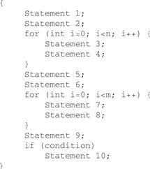
Figure 15.10 A piece of nontrivial code.
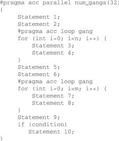
Figure 15.11 Porting is easier with OpenACC (Part 1).
The first pragma in Figure 15.11 creates 32 gangs. Statements 1 and 2 are executed by all gangs. Note that in the original code, these statements are executed only once. However, after the annotation, the compiler will generate code that executes these statements 32 times. This is equivalent to moving a statement into a loop. As long as the statement can be executed extra times without producing incorrect results, this is not a problem.
The second pragma in Figure 15.11 assigns the work of the for loop to the 32 gangs. Each gang will further distribute its share of the work to multiple workers. The exact number of workers in each gang will likely be decided at runtime when the number of iterations and the number of execution units are known.
If statements 1, 2, 5, 6, 9, and 10 can only be executed once, then you can still make the annotations shown in Figure 15.12. In this case, only one gang with 32 workers will be created. The gang leader will execute statements 1, 2, 5, 6, 9, and 10. It will assign the work for the two for loops to its 32 workers. Obviously, the number of workers will be much lower than the previous case, which employs 32 gangs, each of which has multiple workers.
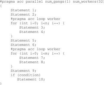
Figure 15.12 Porting is easier with OpenACC (Part 2).
The important point here is that to achieve the same effect with CUDA, more significant code changes are required between the two cases. In the first case, statements 1 and 2 need to be pushed into the loop so that a kernel can be formed with statements 1, 2, 3, and 4. Similarly, another kernel needs to be formed with statements 5, 6, 7, 8, 9, and 10. In the second case, statements 1, 2, 5, 6, 9, and 10 will remain as the host code, whereas statements 1 and 2 will form a kernel and statements 7 and 8 will form a second kernel. We leave the detailed implementation of the kernels in both cases as exercises.
Vector Loop
Recall that OpenACC was designed to support multiple levels of parallelism found in a typical accelerator. The vector clause on a loop construct is often used to express the innermost vector or SIMD (single instruction, multiple data) mode loop in an accelerator region, as illustrated in Figure 15.13.
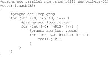
Figure 15.13 Using the vector clause.
On a GPU, a possible implementation is to map a gang to a CUDA block, a worker to a CUDA warp, and a vector element to a thread within a warp. However, this is not mandated by the OpenACC specification and an implementation (compiler/runtime) may choose a different mapping based on the code pattern within an accelerator region for best performance.
Kernels Construct
Prescriptive Versus Descriptive
Like the parallel construct, the kernels construct also allows a programmer to specify which part of a program he or she wants to be executed on an accelerator. And a loop construct can be used inside a kernels construct. One major difference between the two is that a kernels region may be broken into a sequence of kernels, each of which will be executed on the accelerator, while the whole parallel region will become a kernel and be executed on the accelerator. Typically, each loop nest in a kernels construct may become a kernel, as illustrated in Figure 15.14.

Figure 15.14 A kernels region may be broken into a sequence of kernels.
In the figure, the kernels region may be broken into three kernels, one for each loop, and they will be executed on the accelerator in order. It is also possible that some implementations may decide not to generate a kernel for the k loop and therefore this kernels region will contain two kernels—one for the i loop and the j loop each and the k loop is executed on the host.
A kernels region may contain multiple kernels and each may use a different number of gangs, a different number of workers, and different vector lengths. Therefore, there is no num_gangs, num_workers, or vector_length clause on the kernels construct. You can specify them on the enclosed loop construct if you want to, as illustrated in Figure 15.14.
Now let’s take a look at another major difference between the parallel construct and the kernels construct. In Figure 15.14, how many times will the k loop be executed? Previously we’ve learned that the non-work-sharing code inside a parallel construct will be executed redundantly by the gang leads (see Figures 15.5 and 15.6). If the k loop in Figure 15.14 were inside a parallel construct, then the statement d[k] = c[k] is executed 2,048 times the number of gangs. This is different in a kernels construct, in which case it is just 2,048 times.
The parallel construct and the kernels construct were designed from two different perspectives. The kernels construct is more descriptive. It describes the intention of the programmer. The compiler is responsible for mapping and partitioning the program to the underlying hardware. Notice we use the word “may” when we explain the kernels code in Figure 15.14. It is possible that an OpenACC-compliant compiler decides not to generate any kernels at all for the kernels region in Figure 15.14. The loop constructs used for the i and j loops tells the compiler to generate such code that the loop iterations will be shared among the gang leaders only if the compiler decides to generate kernels for these loops. There are two common reasons why a compiler decides not to generate a kernel for a loop construct. One reason is safety. The compiler checks whether parallelizing the loop will give the same execution result as the sequential version does. A series of analyses will be performed on the loop and the rest of the program. If the compiler finds it is not safe to parallelize the loop or cannot decide whether it is safe due to lack of information, then the compiler will not parallelize the loop and hence will not generate a kernel for the loop construct. The other reason is performance. The ultimate goal for using OpenACC directive is to get speedup. The compiler may decide not to parallelize and execute a loop on the accelerator if it finds doing so will only slow down the program. Since the compiler will mostly take care of the parallelization issues, the descriptive approach makes porting programs to OpenACC relatively easier. The downside is the quality of the generated accelerated code depends significantly on the capability of the compiler used. A high-quality compiler is expected to give feedbacks to the programmer on how it compiles kernels constructs and why it does not parallelize certain loops. With this information, the programmer can be sure whether his or her intension is achieved and may provide more hints to the compiler to achieve his or her goal. In the next section, we will show a few ways to help an OpenACC compiler.
The parallel construct is more prescriptive. The compiler does what the programmer instructs it to do. The programmer ultimately has more control of where to generate kernels and how to parallelize and schedule loops. Different OpenACC compilers should perform the similar transformations to a parallel construct. The downside is that there is no safety net. If a loop has data dependence between different iterations and is unsafe to be parallelized, then a programmer should not put such a serial loop inside a loop construct. This is the same philosophy taken by OpenMP, which is another successful directive-based approach for parallel programming. Programmers who are familiar with OpenMP should feel comfortable using parallel constructs.
Ways to Help an OpenACC Compiler
To parallelize a loop inside a kernels region, an OpenACC compiler generally needs to prove there is no cross-iteration data dependence in the loop. There is no data dependence in the i loop in Figure 15.15. All iterations can be executed in parallel and give the same result as when the iterations are executed sequentially. An OpenACC compiler should have no trouble deciding the i loop is parallelizable. In the j loop, each iteration uses the value of array element a[] defined in the previous iteration, therefore, the result will be different if the loops are executed in parallel. An OpenACC compiler should have no trouble deciding the ‘j’ loop is not parallelizable.
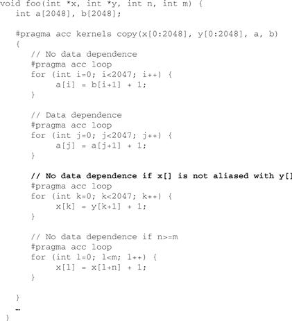
Figure 15.15 Data dependence.
For the k loop, there is no data dependence if x[] and y[] are not aliased. However, this cannot be decided by examining the function foo() alone. If an OpenACC compiler does not perform interprocedural analysis or the call site of function foo() is not available, then the compiler has to conservatively assume there is data dependence. If x[] and y[] are indeed never aliased, we can add the C restrict qualifier to the declaration of pointer argument x and y as illustrated in Figure 15.16. An OpenACC compiler should then be able to use this information to decide if the k loop is parallelizable.
![]()
Figure 15.16 Use restrict qualifier to specify no alias.
Now what to do with the 1 loop? This loop is parallelizable if the value of n is no less than m. Let’s assume this is always true in this program. However, there is no C language construct to express such information. In this case, we can add an independent clause to the loop construct, as illustrated in Figure 15.17. The independent clause simply tells the compiler that the associated loop is parallelizable and no analysis is required. You can also add the independent clause to the ‘i’. You could also add the clause to the ‘j’ loop construct, but that would not be correct.
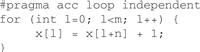
Figure 15.17 Use the ‘independent’ clause to declare a loop is parallelizable.
Data Management
Data Clauses
So far you have seen copy, copyin, and copyout clauses used on parallel and kernels constructs. These are called data clauses. A data clause has a list of arguments separated by a comma. Each argument can be a variable name or a subarray specification. The OpenACC compiler and runtime will create a copy of the variable or subarray in the device memory. Reference to the variable or subarray within the parallel or kernels constructs will be made to the device copy.
The code snippet in Figure 15.18 is from the matrix multiplication example in Figure 15.4. Here, three pieces of memory are allocated on the device. Arrays M and N are the input data, so they are declared as copyin. The copyin from the host memory to the device memory happens right before the parallel region starts execution. Array P is the output data, so it is declared as copyout. The copyout from the device memory to the host memory happens right after the parallel region ends. The copy clause can be used to declare data that needs to be both copied in and copied out.
![]()
Figure 15.18 Data clauses used in Figure 15.4.
Notice that the subarray specification is used for M, N, and P here. That’s because M, N, and P are actually pointers and we need to specify the range of memory that needs to be copied. The value before and after the : specifies the starting array element and the number of array elements, respectively. So M[0:Mh∗Mw] means M[0], M[1], M[2], …, and M[Mh∗Mw-1]. A common programmer error is mistaking the second value as the last array element.
Some variables do not need to be copied in or copyied out—their values are generated and consumed within a kernel. In such cases, the create clause can be used.
Another commonly used data clause is the deviceptr clause. This clause takes a list of pointers as its argument and declares that these are actually device pointers so that the data does not need to be allocated or moved between the host and the device for memory pointed by these pointers. When a program uses both OpenACC and CUDA kernels (or CUDA libraries, such as cuFFT, cuBLAS, etc.), the deviceptr clause becomes handy. Figure 15.19 shows an example of doing the matrix multiplication twice, first using a CUDA kernel and then using an OpenACC parallel region—both work on the same device memory allocated by cudaMalloc().
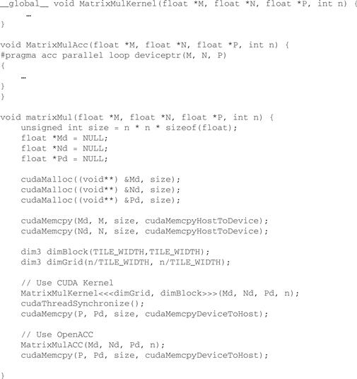
Figure 15.19 Use deviceptr to pass cudaMalloc() data to OpenACC parallel or kernels region.
Data Construct
In OpenACC, host memory and device memory are separated. Data transfer between the host and the accelerator can play a significant role in the overall performance of an OpenACC application. For example, when a computationally intense loop nest of an iterative solver, implemented using a parallel loop, transfers data back and forth between host and the accelerator at every iteration, then there may be a loss of performance. The OpenACC data construct allows one to exploit reuse by avoiding data transfers during multiple executions of parallel or kernels regions.
Figure 15.20 shows a simplified implementation of a 2D Jacobi relaxation. Each element in the array field is updated by taking the average of each element with its eight neighbors. This is repeated 256 times. Another array tmpfield is used to make the relaxation parallel. In each pass, the values are read from one array and the average is computed and then it is written into the same position in the second array. Since the two arrays do not overlap, the updates are completely data parallel. Lines 6-24 implement one pass of the relaxation. Each pass is executed in an OpenACC parallel region. We group the 256 passes into 128 pairs. Each pair contains two parallel regions—one updates tmpfield with field, and the other updates field with tmpfield. Recall that there is no synchronization between gangs. Therefore, we need two parallel constructs to make sure the writes to one array are completed before the array can be used as the source of updates in the next pass.
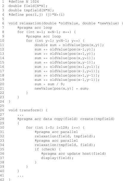
Figure 15.20 Use of data and update constructs.
We want the data to stay on the device during all the 256 passes. This is achieved by using the data construct in line 28. The data region specified by the data construct is from line 30-38, including all called functions. The copy(field) clause says we need to create a device copy of array field, copy its data from the host to the device when the data region starts, and copy its data back to the host when the data region ends. And for the enclosed parallel constructs at lines 31 and 33, just use this copy of field. The create(tmpfield) clause says we need to create a device copy of array tmpfield for this data region, and use this copy for the enclosed parallel constructs at lines 31 and 33.
Now the data is on the device all the time during the passes. What if we want to check the intermediate result on the host occasionally? We can do it by using the update directive, as illustrated at line 36. This says the value of the host array ‘fields’ should be updated with that of the device copy at this point. Since the update is performed conditionally in the code, the data transfer won’t happen if not required. The update directive can also be used to update the value of the device copy with that of the host copy.
Asynchronous Computation and Data Transfer
OpenACC provides support for asynchronous computation and data transfer. An async clause can be added to parallel, kernels, or update directive to enable asynchronous execution. If there is no async clause, the host process will wait until the parallel region, kernels region, or updates are complete before continuing. If there is an async clause, the host process will continue with the code following the directive when the parallel region, kernels region, or updates are processed asynchronously. An asynchronous event can be waited by using the wait directive or OpenACC runtime library routines.
In the Jacobi relaxation example in Figure 15.20, the update of the host copy of field (line 37) and the display of it on the host could happen in parallel with the compute of tmpfield (lines 31 and 32) on the device.
In Figure 15.21, to enable the asynchronous execution, we move the update and display in between the two parallel regions, add an async clause to the parallel directive at line 31, and add a wait directive before the second parallel directive at line 33.
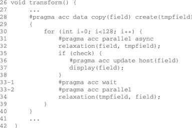
Figure 15.21 async and wait.
We can replace the wait directive with a call to the OpenACC acc_async_wait_all() routine and achieve the same effect. OpenACC provides a richer set of routines to support the asynchronous wait functionality, including the capability to test whether an asynchronous activity has completed rather than just waiting for its completion.
15.5 Future Directions of OpenACC
We believe using OpenACC will become a promising and effective approach to port existing applications to accelerators and even write accelerated applications from scratch. The following are a few directions we see the OpenACC programming model going in.
• Be more general. The current OpenACC model and implementations have quite a few limitations, such as function calls must be able to be in-lined, no support for dynamic memory allocation on the device, etc. It is due to the fact that most OpenACC features were originally designed at the CUDA 3.0 timeframe. Since then, more software and hardware features have been developed on the CUDA platform. For example, in CUDA 4.0, GPUs can be shared across multiple threads, and C++ new/delete and virtual functions support are added. In CUDA 5.0, separate compilation and device code linking is available. OpenACC will certainly take advantage of these new technologies to make the program model more general.
• Integrated with OpenMP. OpenMP and OpenACC both use the directive approach to parallel programming. OpenMP has traditionally been focusing on shared memory systems. The OpenMP ARB has formed an accelerator working group to extend OpenMP support on accelerators. All OpenACC founding members are members of this working group. These members intend to merge the two specifications to create a common one.
Last but not least, we encourage you to follow the latest development of OpenACC by visiting the official OpenACC web site at openacc.org. Besides the latest update to the specification itself, the web site provides a rich resource for documents, FAQs, tutorials, code samples, vendor news, and discussion forums.
15.6 Exercises
15.1. In the following parallel region, how many instances of statement 1 will be executed in total?
#pragma acc parallel gang(1024) worker(32)
{
#pragma acc loop worker
for (int i=0; i<2048; i++) {
statement 1;
}
}
15.2. What are the two major differences between the parallel construct and the kernels construct?
15.3. Implement the matrix multiplication using the kernels construct.
15.4. Reimplement Jacobi relaxation using the kernels constructs. Use a different number of gangs, works, and vector lengths to see how they affect performance.