
Chapter 8
Parallel Patterns: Convolution
With an Introduction to Constant Memory and Caches
Chapter Outline
8.1 Background
8.2 1D Parallel Convolution—A Basic Algorithm
8.3 Constant Memory and Caching
8.4 Tiled 1D Convolution with Halo Elements
8.5 A Simpler Tiled 1D Convolution—General Caching
8.6 Summary
8.7 Exercises
In the next several chapters, we will discuss a set of important parallel computation patterns. These patterns are the basis of many parallel algorithms that appear in applications. We will start with convolution, which is a popular array operation that is used in various forms in signal processing, digital recording, image processing, video processing, and computer vision. In these application areas, convolution is often performed as a filter that transforms signals and pixels into more desirable values. For example, Gaussian filters are convolution filters that can be used to sharpen boundaries and edges of objects in images. Other filters smooth out the signal values so that one can see the big-picture trend. They also form the basis of a large number of force and energy calculation algorithms used in simulation models. Convolution typically involves a significant number of arithmetic operations on each data element. For large data sets such as high-definition images and videos, the amount of computation can be very large. Each output data element can be calculated independently of each other, a desirable trait for massively parallel computing. On the other hand, there is a substantial level of input data sharing among output data elements with somewhat challenging boundary conditions. This makes convolution an important use case of sophisticated tiling methods and input data staging methods.
8.1 Background
Mathematically, convolution is an array operation where each output data element is a weighted sum of a collection of neighboring input elements. The weights used in the weighted sum calculation are defined by an input mask array, commonly referred to as the convolution kernel. Since there is an unfortunate name conflict between the CUDA kernel functions and convolution kernels, we will refer to these mask arrays as convolution masks to avoid confusion. The same convolution mask is typically used for all elements of the array.
In audio digital signal processing, the input data are in 1D form and represent signal volume as a function of time. Figure 8.1 shows a convolution example for 1D data where a five-element convolution mask array M is applied to a seven-element input array N. We will follow the C language convention where N and P elements are indexed from 0 to 6 and M elements are indexed from 0 to 4. The fact that we use a five-element mask M means that each P element is generated by a weighted sum of the corresponding N element, up to two elements to the left and up to two elements to the right. For example, the value of P[2] is generated as the weighted sum of N[0] (N[2-2]) through N[4] (N[2+2]). In this example, we arbitrarily assume that the values of the N elements are 1, 2, 3, …, 7. The M elements define the weights, the values of which are 3, 4, 5, 4, and 3 in this example. Each weight value is multiplied to the corresponding N element values before the products are summed together. As shown in Figure 8.1, the calculation for P[2] is as follows:
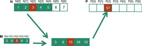
Figure 8.1 A 1D convolution example, inside elements.
P[2] = N[0]∗M[0] + N[1]∗M[1] + N[2]∗M[2] + N[3]∗M[3] + N[4]∗M[4]
= 1∗3 + 2∗4 + 3∗5 + 4∗4 + 5∗3
= 57
In general, the size of the mask tends to be an odd number, which makes the weighted sum calculation symmetric around the element being calculated. That is, an odd number of mask elements define the weight to be applied to the input element in the corresponding position of the output element along with the same number of input elements on each side of that position. In Figure 8.1, with a mask size of five elements, each output element is calculated as the weighted sum of the corresponding input element, two elements on the left and two elements on the right. For example, P[2] is calculated as the weighted sum of N[2] along with N[0] and N[1] on the left and N[3] and N[4] on the right.
In Figure 8.1, the calculation for P element P[i] can be viewed as an inner product between the subarray of N that starts at N[i-2] and the M array. Figure 8.2 shows the calculation for P[3]. The calculation is shifted by one N element from that of Figure 8.1. That is the value of P[3] is the weighted sum of N[1] (N[3-2]) through N[5] (3+2). We can think of the calculation for P[3] as follows:
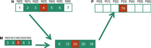
Figure 8.2 1D convolution, calculation of P[3].
P[3] = N[1]∗M[0] + N[2]∗M[1] + N[3]∗M[2] + N[4]∗M[3] + N[5]∗M[4]
= 2∗3 + 3∗4 + 4∗5 + 5∗4 + 6∗3
= 76
Because convolution is defined in terms of neighboring elements, boundary conditions naturally exist for output elements that are close to the ends of an array. As shown in Figure 8.3, when we calculate P[1], there is only one N element to the left of N[1]. That is, there are not enough N elements to calculate P[1] according to our definition of convolution. A typical approach to handling such a boundary condition is to define a default value to these missing N elements. For most applications, the default value is 0, which is what we use in Figure 8.3. For example, in audio signal processing, we can assume that the signal volume is 0 before the recording starts and after it ends. In this case, the calculation of P[1] is as follows:
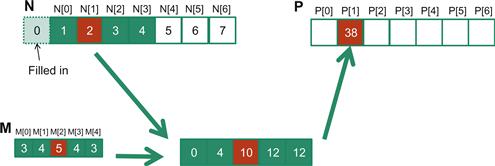
Figure 8.3 1D convolution boundary condition.
P[1] = 0 ∗ M[0] + N[0]∗M[1] + N[1]∗M[2] + N[2]∗M[3] + N[3]∗M[4]
= 0 ∗ 3 + 1∗4 + 2∗5 + 3∗4 + 4∗3
= 38
The N element that does not exist in this calculation is illustrated as a dashed box in Figure 8.3. It should be clear that the calculation of P[0] will involve two missing N elements, both of which will be assumed to be 0 for this example. We leave the calculation of P[0] as an exercise. These missing elements are typically referred to as ghost elements in literature. There are also other types of ghost elements due to the use of tiling in parallel computation. These ghost elements can have significant impact on the complexity and/or efficiency of tiling. We will come back to this point soon.
For image processing and computer vision, input data is usually in 2D form, with pixels in an x-y space. Image convolutions are also two dimensional, as illustrated in Figure 8.4. In a 2D convolution, the mask M is a 2D array. Its x and y dimensions determine the range of neighbors to be included in the weighted sum calculation. In Figure 8.4, we use a 5×5 mask for simplicity. In general, the mask does not have to be a square array. To generate an output element, we take the subarray of which the center is at the corresponding location in the input array N. We then perform pairwise multiplication between elements of the mask array and those of the mask array. For our example, the result is shown as the 5×5 product array below N and P arrays in Figure 8.4. The value of the output element is the sum of all elements of the product array.

Figure 8.4 A 2D convolution example.
The example in Figure 8.4 shows the calculation of P2,2. For brevity, we will use Ny,x to denote N[y][x] in addressing a C array. Since N and P are most likely dynamically allocated arrays, we will be using linearized indices in our actual code examples. The subarray of N for calculating the value of P2,2 span from N0,0 to N0,4 in the x or horizontal direction and N0,0 to N4,0 in the y or vertical direction. The calculation is as follows:
P2,2 = N0,0∗M0,0 + N0,1∗M0,1 + N0,2∗M0,2 + N0,3∗M0,3 + N0,4∗M0,4
+ N1,0∗M1,0 + N1,1∗M1,1 + N1,2∗M1,2 + N1,3∗M1,3 + N1,4∗M1,4
+ N2,0∗M2,0 + N2,1∗M2,1 + N2,2∗M2,2 + N2,3∗M2,3 + N2,4∗M2,4
+ N3,0∗M3,0 + N3,1∗M3,1 + N3,2∗M3,2 + N3,3∗M3,3 + N3,4∗M3,4
+ N4,0∗M4,0 + N4,1∗M4,1 + N4,2∗M4,2 + N4,3∗M4,3 + N4,4∗M4,4
= 1∗1 + 2∗2 + 3∗3 + 4∗2 + 5∗1
+ 2∗2 + 3∗3 + 4∗4 + 5∗3 + 6∗2
+ 3∗3 + 4∗4 + 5∗5 + 6∗4 + 7∗3
+ 5∗1 + 6∗2 + 7∗3 + 8∗2 + 5∗1
= 1 + 4 + 9 + 8 + 5
+ 4 + 9 + 16 + 15 + 12
+ 9 + 16 + 25 + 24 + 21
+ 8 + 15 + 24 + 21 + 16
+ 5 + 12 + 21 + 16 + 5
= 321
Like 1D convolution, 2D convolution must also deal with boundary conditions. With boundaries in both the x and y dimensions, there are more complex boundary conditions: the calculation of an output element may involve boundary conditions along a horizontal boundary, a vertical boundary, or both. Figure 8.5 illustrates the calculation of a P element that involves both boundaries. From Figure 8.5, the calculation of P1,0 involves two missing columns and one missing horizontal row in the subarray of N. Like in 1D convolution, different applications assume different default values for these missing N elements. In our example, we assume that the default value is 0. These boundary conditions also affect the efficiency of tiling. We will come back to this point soon.
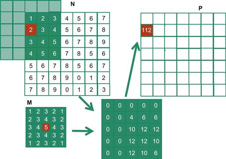
Figure 8.5 A 2D convolution boundary condition.
8.2 1D Parallel Convolution—A Basic Algorithm
As we mentioned in Section 8.1, the calculation of all output (P) elements can be done in parallel in a convolution. This makes convolution an ideal problem for parallel computing. Based on our experience in matrix–matrix multiplication, we can quickly write a simple parallel convolution kernel. For simplicity, we will work on 1D convolution.
The first step is to define the major input parameters for the kernel. We assume that the 1D convolution kernel receives five arguments: pointer to input array N, pointer to input mask M, pointer to output array P, size of the mask Mask_Width, and size of the input and output arrays Width. Thus, we have the following set up:
__global__ void convolution_1D_basic_kernel(float ∗N, float ∗M, float ∗P,
int Mask_Width, int Width) {
// kernel body
}
The second step is to determine and implement the mapping of threads to output elements. Since the output array is one dimensional, a simple and good approach is to organize the threads into a 1D grid and have each thread in the grid calculate one output element. Readers should recognize that this is the same arrangement as the vector addition example as far as output elements are concerned. Therefore, we can use the following statement to calculate an output element index from the block index, block dimension, and thread index for each thread:
int i = blockIdx.x∗blockDim.x + threadIdx.x;
Once we determined the output element index, we can access the input N elements and the mask M elements using offsets to the output element index. For simplicity, we assume that Mask_Width is an odd number and the convolution is symmetric, that is, Mask_Width is 2∗n+1 where n is an integer. The calculation of P[i] will use N[i-n], N[i-n+1],…, N[i-1], N[i], N[i+1], …, N[i+n-1], N[i+n]. We can use a simple loop to do this calculation in the kernel:
float Pvalue = 0;
int N_start_point = i - (Mask_Width/2);
for (int j = 0; j < Mask_Width; j++) {
if (N_start_point + j >= 0 && N_start_point + j < Width) {
Pvalue += N[N_start_point + j]∗M[j];
}
}
The variable Pvalue will allow all intermediate results to be accumulated in a register to save DRAM bandwidth. The for loop accumulates all the contributions from the neighboring elements to the output P element. The if statement in the loop tests if any of the input N elements used are ghost elements, either on the left side or the right side of the N array. Since we assume that 0 values will be used for ghost elements, we can simply skip the multiplication and accumulation of the ghost element and its corresponding N element. After the end of the loop, we release the Pvalue into the output P element. We now have a simple kernel in Figure 8.6.
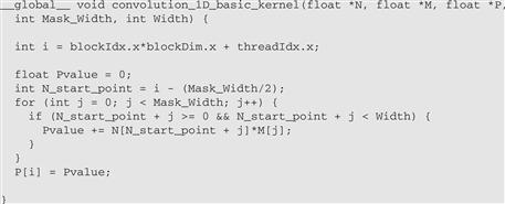
Figure 8.6 A 1D convolution kernel with boundary condition handling.
We can make two observations about the kernel in Figure 8.6. First, there will be control flow divergence. The threads that calculate the output P elements near the left end or the right end of the P array will handle ghost elements. As we showed in Section 8.1, each of these neighboring threads will encounter a different number of ghost elements. Therefore, they will all be somewhat different decisions in the if statement. The thread that calculates P[0] will skip the multiply-accumulate statement about half of the time, whereas the one that calculates P[1] will skip one fewer times, and so on. The cost of control divergence will depend on Width, the size of the input array, and Mask_Width (the size of the masks). For large input arrays and small masks, the control divergence only occurs to a small portion of the output elements, which will keep the effect of control divergence small. Since convolution is often applied to large images and spatial data, we typically expect that the effect of convergence will be modest or insignificant.
A more serious problem is memory bandwidth. The ratio of floating-point arithmetic calculation to global memory accesses is only about 1.0 in the kernel. As we have seen in the matrix–matrix multiplication example, this simple kernel can only be expected to run at a small fraction of the peak performance. We will discuss two key techniques for reducing the number of global memory accesses in the next two sections.
8.3 Constant Memory and Caching
We can make three interesting observations about the way the mask array M is used in convolution. First, the size of the M array is typically small. Most convolution masks are less than 10 elements in each dimension. Even in the case of a 3D convolution, the mask typically contains only less than 1,000 elements. Second, the contents of M are not changed throughout the execution of the kernel. Third, all threads need to access the mask elements. Even better, all threads access the M elements in the same order, starting from M[0] and move by one element a time through the iterations of the for loop in Figure 8.6. These two properties make the mask array an excellent candidate for constant memory and caching.
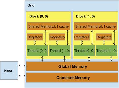
Figure 8.7 A review of the CUDA memory model.
The CUDA programming model allows programmers to declare a variable in the constant memory. Like global memory variables, constant memory variables are also visible to all thread blocks. The main difference is that a constant memory variable cannot be changed by threads during kernel execution. Furthermore, the size of the constant memory can vary from device to device. The amount of constant memory available on a device can be learned with a device property query. Assume that dev_prop is returned by cudaGetDeviceProperties(). The field dev_prop.totalConstMem indicates the amount of constant memory available on a device is in the field.
To use constant memory, the host code needs to allocate and copy constant memory variables in a different way than global memory variables. To declare an M array in constant memory, the host code declares it as a global variable as follows:
#define MAX_MASK_WIDTH 10
__constant__ float M[MAX_MASK_WIDTH];
This is a global variable declaration and should be outside any function in the source file. The keyword __constant__ (two underscores on each side) tells the compiler that array M should be placed into the device constant memory.
Assume that the host code has already allocated and initialized the mask in a mask h_M array in the host memory with Mask_Width elements. The contents of the h_M can be transferred to M in the device constant memory as follows:
cudaMemcpyToSymbol(M, h_M, Mask_Width∗sizeof(float));
Note that this is a special memory copy function that informs the CUDA runtime that the data being copied into the constant memory will not be changed during kernel execution. In general, the use of the cudaMemcpyToSymbol() function is as follows:
cudaMemcpyToSymbol(dest, src, size)
where dest is a pointer to the destination location in the constant memory, src is a pointer to the source data in the host memory, and size is the number of bytes to be copied.
Kernel functions access constant memory variables as global variables. Thus, their pointers do not need to be passed to the kernel as parameters. We can revise our kernel to use the constant memory as shown in Figure 8.8. Note that the kernel looks almost identical to that in Figure 8.6. The only difference is that M is no longer accessed through a pointer passed in as a parameter. It is now accessed as a global variable declared by the host code. Keep in mind that all the C language scoping rules for global variables apply here. If the host code and kernel code are in different files, the kernel code file must include the relevant external declaration information to ensure that the declaration of M is visible to the kernel.
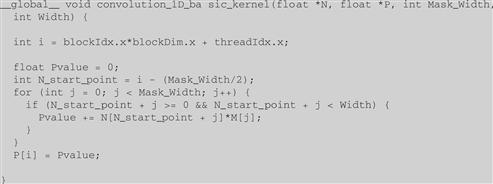
Figure 8.8 A 1D convolution kernel using constant memory for M.
Like global memory variables, constant memory variables are also located in DRAM. However, because the CUDA runtime knows that constant memory variables are not modified during kernel execution, it directs the hardware to aggressively cache the constant memory variables during kernel execution. To understand the benefit of constant memory usage, we need to first understand more about modern processor memory and cache hierarchies.
In modern processors, accessing a variable from DRAM takes hundreds if not thousands of clock cycles. Also, the rate at which variables can be accessed from DRAM is typically much lower than the rate at which processors can perform an arithmetic operation. The long latency and limited bandwidth of DRAM has been a major bottleneck in virtually all modern processors commonly referred to as the memory wall. To mitigate the effect of memory bottleneck, modern processors commonly employ on-chip cache memories, or caches, to reduce the number of variables that need to be accessed from DRAM (Figure 8.9).
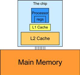
Figure 8.9 A simplified view of the cache hierarchy of modern processors.
Unlike CUDA shared memory, or scratchpad memories in general, caches are “transparent” to programs. That is, to use CUDA shared memory, a program needs to declare variables as __shared__ and explicitly move a global memory variable into a shared memory variable. On the other hand, when using caches, the program simply accesses the original variables. The processor hardware will automatically retain some of the most recently or frequently used variables in the cache and remember their original DRAM address. When one of the retained variables is used later, the hardware will detect from their addresses that a copy of the variable is available in the cache. The value of the variable will then be provided from the cache, eliminating the need to access DRAM.
There is a trade-off between the size of a memory and the speed of a memory. As a result, modern processors often employ multiple levels of caches. The numbering convention for these cache levels reflects the distance to the processor. The lowest level, L1 or level 1, is the cache that is directly attached to a processor core. It runs at a speed very close to the processor in both latency and bandwidth. However, an L1 cache is small in size, typically between 16 KB and 64 KB. L2 caches are larger, in the range of 128 KB to 1 MB, but can take tens of cycles to access. They are typically shared among multiple processor cores, or streaming multiprocessors (SMs) in a CUDA device. In some high-end processors today, there are even L3 caches that can be of several MB in size.
A major design issue with using caches in a massively parallel processor is cache coherence, which arises when one or more processor cores modify cached data. Since L1 caches are typically directly attached to only one of the processor cores, changes in its contents are not easily observed by other processor cores. This causes a problem if the modified variable is shared among threads running on different processor cores. A cache coherence mechanism is needed to ensure that the contents of the caches of the other processor cores are updated. Cache coherence is difficult and expensive to provide in massively parallel processors. However, their presence typically simplifies parallel software development. Therefore, modern CPUs typically support cache coherence among processor cores. While modern GPUs provide two levels of caches, they typically do without cache coherence to maximize hardware resources available to increase the arithmetic throughput of the processor.
Constant memory variables play an interesting role in using caches in massively parallel processors. Since they are not changed during kernel execution, there is no cache coherence issue during the execution of a kernel. Therefore, the hardware can aggressively cache the constant variable values in L1 caches. Furthermore, the design of caches in these processors is typically optimized to broadcast a value to a large number of threads. As a result, when all threads in a warp access the same constant memory variable, as is the case with M, the caches can provide a tremendous amount of bandwidth to satisfy the data needs of threads. Also, since the size of M is typically small, we can assume that all M elements are effectively always accessed from caches. Therefore, we can simply assume that no DRAM bandwidth is spent on M accesses. With the use of constant caching, we have effectively doubled the ratio of floating-point arithmetic to memory access to 2.
The accesses to the input N array elements can also benefit from caching in more recent devices. We will come back to this point in Section 8.5.
8.4 Tiled 1D Convolution with Halo Elements
We now address the memory bandwidth issue in accessing the N array element with a tiled convolution algorithm. Recall that in a tiled algorithm, threads collaborate to load input elements into an on-chip memory and then access the on-chip memory for their subsequent use of these elements. For simplicity, we will continue to assume that each thread calculates one output P element. With up to 1,024 threads in a block we can process up to 1,024 data elements. We will refer to the collection of output elements processed by each block as an output tile. Figure 8.10 shows a small example of a 16-element, 1D convolution using four thread blocks of four threads each. In this example, there are four output tiles. The first output tile covers P[0] through P[3], the second tile P[4] through P[7], the third tile P[8] through P[11], and the fourth tile P[12] through P[15]. Keep in mind that we use four threads per block to keep the example small. In practice, there should be at least 32 threads per block for the current generation of hardware. From this point on, we will assume that M elements are in the constant memory.
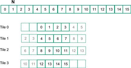
Figure 8.10 A 1D tiled convolution example.
We will discuss two input data tiling strategies for reducing the total number of global memory accesses. The first one is the most intuitive and involves loading all input data elements needed for calculating all output elements of a thread block into the shared memory. The number of input elements to be loaded depends on the size of the mask. For simplicity, we will continue to assume that the mask size is an odd number equal to 2×n+1. That is, each output element P[i] is a weighted sum of the input element at the corresponding input element N[i], the n input elements to the left (N[i-n], …, N[i-1]), and the n input elements to the right (N[i+1], …, N[i+n]). Figure 8.10 shows an example where n=2.
Threads in block 0 calculate output elements P[0] through P[3]. This is the leftmost tile in the output data and is often referred to as the left boundary tile. They collectively require input elements N[0] through N[5]. Note that the calculation also requires two ghost elements to the left of N[0]. This is shown as two dashed empty elements on the left end of tile 0 of Figure 8.6. These ghost elements will be assumed have a default value of 0. Tile 3 has a similar situation at the right end of input array N. In our discussions, we will refer to tiles like tile 0 and tile 3 as boundary tiles since they involve elements at or outside the boundary of the input array N.
Threads in block 1 calculate output elements P[4] through P[7]. They collectively require input elements N[2] through N[9], also shown in Figure 8.10. Calculations for tiles 1 and 2 in Figure 8.10 do not involve ghost elements and are often referred to as internal tiles. Note that elements N[2] and N[3] belong to two tiles and are loaded into the shared memory twice, once to the shared memory of block 0 and once to the shared memory of block 1. Since the contents of shared memory of a block are only visible to the threads of the block, these elements need to be loaded into the respective shared memories for all involved threads to access them. The elements that are involved in multiple tiles and loaded by multiple blocks are commonly referred to as halo elements or skirt elements since they “hang” from the side of the part that is used solely by a single block. We will refer to the center part of an input tile that is solely used by a single block the internal elements of that input tile. Tiles 1 and 2 are commonly referred to as internal tiles since they do not involve any ghost elements at or outside the boundaries of the input array N.
We now show the kernel code that loads the input tile into shared memory. We first declare a shared memory array, N_ds, to hold the N tile for each block. The size of the shared memory array must be large enough to hold the left halo elements, the center elements, and the right halo elements of an input tile. We assume that Mask_Size is an odd number. The total is TILE_SIZE + MAX_MASK_WIDTH -1, which is used in the following declaration in the kernel:
__shared__ float N_ds[TILE_SIZE + MAX_MASK_WIDTH - 1];
We then load the left halo elements, which include the last n = Mask_Width/2 center elements of the previous tile. For example, in Figure 8.10, the left halo elements of tile 1 consist of the last two center elements of tile 0. In C, assuming that Mask_Width is an odd number, the expression Mask_Width/2 will result in an integer value that is the same as (Mask_Width-1)/2. We will use the last (Mask_Width/2) threads of the block to load the left halo element. This is done with the following two statements:
int halo_index_left = (blockIdx.x - 1)∗blockDim.x + threadIdx.x;
if (threadIdx.x >= blockDim.x - n) {
N_ds[threadIdx.x - (blockDim.x - n)] =
(halo_index_left < 0) ? 0 : N[halo_index_left];
In the first statement, we map the thread index to the element index into the previous tile with the expression (blockIdx.x-1)∗blockDim.x+threadIdx.x. We then pick only the last n threads to load the needed left halo elements using the condition in the if statement. For example, in Figure 8.6, blockDim.x equals 4 and n equals 2; only threads 2 and 3 will be used. Threads 0 and 1 will not load anything due to the failed condition.
For the threads used, we also need to check if their halo elements are ghost elements. This can be checked by testing if the calculated halo_index_left value is negative. If so, the halo elements are actually ghost elements since their N indices are negative, outside the valid range of the N indices. The conditional C assignment will choose 0 for threads in this situation. Otherwise, the conditional statement will use the halo_index_left to load the appropriate N elements into the shared memory. The shared memory index calculation is such that left halo elements will be loaded into the shared memory array starting at element 0. For example, in Figure 8.10, blockDim.x-n equals 2. So for block 1, thread 2 will load the leftmost halo element into N_ds[0] and thread 3 will load the next halo element into N_ds[1]. However, for block 0, both threads 2 and 3 will load value 0 into N_ds[0] and N_ds[1].
The next step is to load the center elements of the input tile. This is done by mapping the blockIdx.x and threadIdx.x values into the appropriate N indices, as shown in the following statement. Readers should be familiar with the N index expression used:
N_ds[n + threadIdx.x] = N[blockIdx.x∗blockDim.x + threadIdx.x];
Since the first n elements of the N_ds array already contain the left halo elements, the center elements need to be loaded into the next section of N_ds. This is done by adding n to threadIdx.x as the index for each thread to write its loaded center element into N_ds.
We now load the right halo elements, which is quite similar to loading the left halo. We first map the blockIdx.x and threadIdx.x to the elements of next output tile. This is done by adding (blockIdx.x+1)∗blockDim.x to the thread index to form the N index for the right halo elements. In this case, we are loading the beginning Mask_Width:
int halo_index_right=(blockIdx.x + 1)∗blockDim.x + threadIdx.x;
if (threadIdx.x < n) {
N_ds[n + blockDim.x + threadIdx.x] =
(halo_index_right >= Width) ? 0 : N[halo_index_right];
Now that all the input tile elements are in N_ds, each thread can calculate their output P element value using the N_ds elements. Each thread will use a different section of the N_ds. Thread 0 will use N_ds[0] through N_ds[Mask_Width-1]; thread 1 will use N_ds[1] through N[Mask_Width]. In general, each thread will use N_ds[threadIdx.x] through N[threadIdx.x+Mask_Width-1]. This is implemented in the following for loop to calculate the P element assigned to the thread:
float Pvalue = 0;
for(int j = 0; j < Mask_Width; j++) {
Pvalue += N_ds[threadIdx.x + j]∗M[j];
}
P[i] = Pvalue;
However, one must not forget to do a barrier synchronization using syncthreads() to make sure that all threads in the same block have completed loading their assigned N elements before anyone should start using them from the shared memory.
Note that the code for multiply and accumulate is simpler than the base algorithm. The conditional statements for loading the left and right halo elements have placed the 0 values into the appropriate N_ds elements for the first and last thread block.
The tiled 1D convolution kernel is significantly longer and more complex than the basic kernel. We introduced the additional complexity to reduce the number of DRAM accesses for the N elements. The goal is to improve the arithmetic to memory access ratio so that the achieved performance is not limited or less limited by the DRAM bandwidth. We will evaluate improvement by comparing the number of DRAM accesses performed by each thread block for the kernels in Figure 8.8 and Figure 8.11.
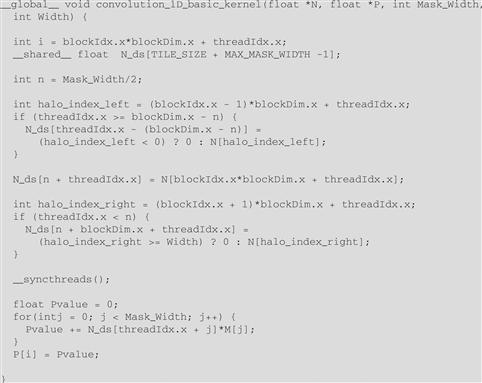
Figure 8.11 A tiled 1D convolution kernel using constant memory for M.
In Figure 8.8, there are two cases. For thread blocks that do not handle ghost elements, the number of N elements accessed by each thread is Mask_Width. Thus, the total number of N elements accessed by each thread block is blockDim.x∗Mask_Width or blockDim.x∗(2n+1). For example, if Mask_Width is equal to 5 and each block contains 1,024 threads, each block accesses a total of 5,120 N elements.
For the first and last blocks, the threads that handle ghost elements, no memory access is done for the ghost elements. This reduces the number of memory accesses. We can calculate the reduced number of memory accesses by enumerating the number of threads that use each ghost element. This is illustrated with a small example in Figure 8.12. The leftmost ghost element is used by one thread. The second left ghost element is used by two threads. In general, the number of ghost elements is n and the number of threads that use each of these ghost elements, from left to right is 1, 2, …, n. This is a simple series with sum n(n + 1)/2, which is the total number of accesses that were avoided due to ghost elements. For our simple example where Mask_Width is equal to 5 and n is equal to 2, the number of accesses avoided due to ghost elements is 2×3/2=3. A similar analysis gives the same results for the right ghost elements. It should be clear that for large thread blocks, the effect of ghost elements for small mask sizes will be insignificant.
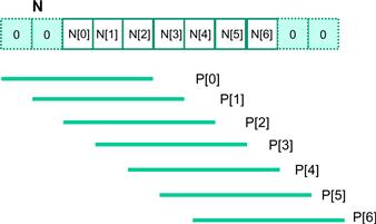
Figure 8.12 A small example of accessing N elements and ghost elements.
We now calculate the total number of memory accesses for N elements by the tiled kernel in Figure 8.11. All the memory accesses have been shifted to the code that loads the N elements into the shared memory. In the tiled kernel, each N element is only loaded by one thread. However, 2n halo elements will also be loaded, n from the left and n from the right, for blocks that do not handle ghost elements. Therefore, we have the blockDim.x+2n elements in for the internal thread blocks and blockDim+n for boundary thread blocks.
For internal thread blocks, the ratio of memory accesses between the basic and the tiled 1D convolution kernel is
(blockDim.x∗(2n+1)) / (blockDim.x+2n)
whereas the ratio for boundary blocks is
(blockDim.x∗(2n+1) − n(n+1)/2) / (blockDim.x+n)
For most situations, blockDim.x is much larger than n. Both ratios can be approximated by eliminating the small terms n(n + 1)/2 and n:
(blockDim.x∗(2n+1)/ blockDim.x = 2n+1 = Mask_Width
This should be quite an intuitive result. In the original algorithm, each N element is redundantly loaded by approximately Mask_Width threads. For example, in Figure 8.12, N[2] is loaded by the five threads that calculate P[2], P[3], P[4], P[5], and P[6]. That is, the ratio of memory access reduction is approximately proportional to the mask size.
However, in practice, the effect of the smaller terms may be significant and cannot be ignored. For example, if blockDim.x is 128 and n is 5, the ratio for the internal blocks is
(128∗11-10) / (128 + 10) = 1398 / 138 = 10.13
whereas the approximate ratio would be 11. It should be clear that as blockDim.x becomes smaller, the ratio also becomes smaller. For example, if blockDim is 32 and n is 5, the ratio for the internal blocks becomes
(32∗11-10) / (32+10) = 8.14
Readers should always be careful when using smaller block and tile sizes. They may result in significantly less reduction in memory accesses than expected. In practice, smaller tile sizes are often used due to an insufficient amount of on-chip memory, especially for 2D and 3D convolution where the amount of on-chip memory needed grows quickly with the dimension of the tile.
8.5 A Simpler Tiled 1D Convolution—General Caching
In Figure 8.11, much of the complexity of the code has to do with loading the left and right halo elements in addition to the internal elements into the shared memory. More recent GPUs such as Fermi provide general L1 and L2 caches, where L1 is private to each SM and L2 is shared among all SMs. This leads to an opportunity for the blocks to take advantage of the fact that their halo elements may be available in the L2 cache.
Recall that the halo elements of a block are also internal elements of a neighboring block. For example, in Figure 8.10, the halo elements N[2] and N[3] of tile 1 are also internal elements of tile 0. There is a significant probability that by the time block 1 needs to use these halo elements, they are already in the L2 cache due to the accesses by block 0. As a result, the memory accesses to these halo elements may be naturally served from the L2 cache without causing additional DRAM traffic. That is, we can leave the accesses to these halo elements in the original N elements rather than loading them into the N_ds. We now present a simpler tiled 1D convolution algorithm that only loads the internal elements of each tile into the shared memory.
In the simpler tiled kernel, the shared memory N_ds array only needs to hold the internal elements of the tile. Thus, it is declared with the TILE_SIZE, rather than TILE_SIZE+Mask_Width-1:
__shared__ float N_ds[TILE_SIZE];
i = blockIdx.x∗blockDim.x+threadIdx.x;
Loading the tile becomes very simple with only one line of code:
N_ds[threadIdx.x] = N[i];
We still need a barrier synchronization before using the elements in N_ds. The loop that calculates P elements, however, becomes more complex. It needs to add conditions to check for use of both halo elements and ghost elements. The ghost elements are handled with the same conditional statement as that in Figure 8.6. The multiply–accumulate statement becomes more complex:
__syncthreads();
int This_tile_start_point = blockIdx.x ∗ blockDim.x;
int Next_tile_start_point = (blockIdx.x + 1) ∗ blockDim.x;
int N_start_point = i - (Mask_Width/2);
float Pvalue = 0;
for (int j = 0; j < Mask_Width; j ++) {
int N_index = N_start_point + j;
if (N_index >= 0 && N_index < Width) {
if ((N_index >= This_tile_start_point)
&& (N_index < Next_tile_start_point)) {
Pvalue += N_ds[threadIdx.x+j-(Mask_Width/2)]∗M[j];
} else {
Pvalue += N[N_index] ∗ M[j];
}
}
}
P[i] = Pvalue;
The variables This_tile_start_point and Next_tile_start_point hold the starting position index of the tile processed by the current block and that of the tile processed by the next in the next block. For example, in Figure 8.10, the value of This_tile_start_point for block 1 is 4 and the value of Next_tile_start_point is 8.
The new if statement tests if the current access to the N element falls within a tile by testing it against This_tile_start_point and Next_tile_start_point. If the element falls within the tile—that is, it is an internal element for the current block—it is accessed from the N_ds array in the shared memory. Otherwise, it is accessed from the N array, which is hopefully in the L2 cache. The final kernel code is shown is Figure 8.13.
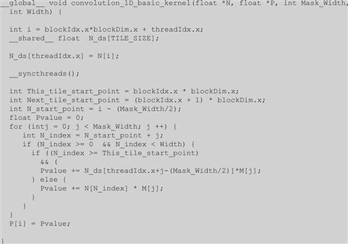
Figure 8.13 A simpler tiled 1D convolution kernel using constant memory and general caching.
Although we have shown kernel examples for only a 1D convolution, the techniques are directly applicable to 2D and 3D convolutions. In general, the index calculation for the N and M arrays are more complex for 2D and 3D convolutions due to higher dimensionality. Also, one will have more loop nesting for each thread since multiple dimensions need to be traversed when loading tiles and/or calculating output values. We encourage readers to complete these higher-dimension kernels as homework exercises.
8.6 Summary
In this chapter, we have studied convolution as an important parallel computation pattern. While convolution is used in many applications such as computer vision and video processing, it also represents a general pattern that forms the basis of many other parallel algorithms. For example, one can view the stencil algorithms in partial differential equation (PDE) solvers as a special case of convolution. For another example, one can also view the calculation of grid point force or the potential value as a special case of convolution.
We have presented a basic parallel convolution algorithm of which the implementations will be limited by DRAM bandwidth for accessing both the input N and mask M elements. We then introduced the constant memory and a simple modification to the kernel and host code to take advantage of constant caching and eliminate practically all DRAM accesses for the mask elements. We further introduced a tiled parallel convolution algorithm that reduces DRAM bandwidth consumption by introducing more control flow divergence and programming complexity. Finally, we presented a simpler tiled parallel convolution algorithm that takes advantage of the L2 caches.
8.7 Exercises
8.1. Calculate the P[0] value in Figure 8.3.
8.2. Consider performing a 1D convolution on array N={4,1,3,2,3} with mask M={2,1,4}. What is the resulting output array?
8.3. What do you think the following 1D convolution masks are doing?
8.4. Consider performing a 1D convolution on an array of size n with a mask of size m:
a. How many halo cells are there in total?
b. How many multiplications are performed if halo cells are treated as multiplications (by 0)?
c. How many multiplications are performed if halo cells are not treated as multiplications?
8.5. Consider performing a 2D convolution on a square matrix of size n×n with a square mask of size m×m:
a. How many halo cells are there in total?
b. How many multiplications are performed if halo cells are treated as multiplications (by 0)?
c. How many multiplications are performed if halo cells are not treated as multiplications?
8.6. Consider performing a 2D convolution on a rectangular matrix of size n1×n2 with a rectangular mask of size m1×m2:
a. How many halo cells are there in total?
b. How many multiplications are performed if halo cells are treated as multiplications (by 0)?
c. How many multiplications are performed if halo cells are not treated as multiplications?
8.7. Consider performing a 1D tiled convolution with the kernel shown in Figure 8.11 on an array of size n with a mask of size m using a tile of size t.
a. How many blocks are needed?
b. How many threads per block are needed?
c. How much shared memory is needed in total?
d. Repeat the same questions if you were using the kernel in Figure 8.13.
8.8. Revise the 1D kernel in Figure 8.6 to perform 2D convolution. Add more width parameters to the kernel declaration as needed.
8.9. Revise the tiled 1D kernel in Figure 8.8 to perform 2D convolution. Keep in mind that the host code also needs to be changed to declare a 2D M array in the constant memory. Pay special attention to the increased usage of shared memory. Also, the N_ds needs to be declared as a 2D shared memory array.
8.10. Revise the tiled 1D kernel in Figure 8.11 to perform 2D convolution. Keep in mind that the host code also needs to be changed to declare a 2D M array in the constant memory. Pay special attention to the increased usage of shared memory. Also, the N_ds needs to be declared as a 2D shared memory array.