5
Introduction to R
R is an extraordinarily powerful open source software program built for working with data. It is one of the most popular data science tools because of its ability to efficiently perform statistical analysis, implement machine learning algorithms, and create data visualizations. R is the primary programming language used throughout this book, and understanding its foundational operations is key to being able to perform more complex tasks.
5.1 Programming with R
R is a statistical programming language that allows you to write code to work with data. It is an open source programming language, which means that it is free and continually improved upon by the R community. The R language has a number of capabilities that allow you to read, analyze, and visualize data sets.
Fun Fact
R is called “R” in part because it was inspired by the language “S,” a language for Statistics developed by AT&T, and because it was developed by Ross Ihaka and Robert Gentleman.
In previous chapters, you leveraged formal language to give instructions to your computer, such as by writing syntactically precise instructions at the command line. Programming in R works in a similar manner: you write instructions using R’s special language and syntax, which the computer interprets as instructions for how to work with data.
However, as projects grow in complexity, it becomes useful if you can write down all the instructions in a single place, and then order the computer to execute all of those instructions at once. This list of instructions is called a script. Executing or “running” a script will cause each instruction (line of code) to be run in order, one after the other, just as if you had typed them in one by one. Writing scripts allows you to save, share, and reuse your work. By saving instructions in a file (or set of files), you can easily check, change, and re-execute the list of instructions as you figure out how to use data to answer questions. And, because R is an interpreted language, rather than a compiled language like C or Java, R programming environments give you the ability to separately execute each individual line of code in your script if you desire.
As you begin working with data in R, you will be writing multiple instructions (lines of code) and saving them in files with the .R extension, representing R scripts. You can write this R code in any text editor (such as Atom), but we recommend you usually use RStudio, a program that is specialized for writing and running R scripts.
5.2 Running R Code
There are a few different ways in which you can have your computer execute code that you write in the R language. The most user-friendly approach is to use RStudio.
5.2.1 Using RStudio
RStudio is an open source integrated development environment (IDE) that provides an informative user interface for interacting with the R interpreter. Generally speaking, IDEs provide a platform for writing and executing code, including viewing the results of the code you have run. This is distinct from a code editor (like Atom), which is used just to write code.
When you open the RStudio program, you will see an interface similar to that in Figure 5.1. An RStudio session usually involves four sections (“panes”), though you can customize this layout if you wish:
Script: The top-left pane is a simple text editor for writing your
Rcode as different script files. While it is not as robust as a text editing program like Atom, it will colorize code, auto-complete text, and allow you to easily execute your code. Note that this pane is hidden if there are no open scripts; selectFile > New File > R Scriptfrom the menu to create a new script file.To execute (run) the code you write, you have two options:
You can execute a section of your script by selecting (highlighting) the desired code and clicking the “Run” button (or use the keyboard shortcut1:
cmd+enteron Mac, orctrl+enteron Windows). If no lines are selected, this will run the line currently containing the cursor. This is the most common way to execute code in RStudio.1RStudio Keyboard Shortcuts: https://support.rstudio.com/hc/en-us/articles/200711853-Keyboard-Shortcuts
Tip
Use
cmd+a(Mac) orctrl+a(Windows) to select the entire script!You can execute an entire script by clicking the “Source” button (at the top right of the Script pane, or via
shift+cmd+enter) to execute all lines of code in the script file, one at a time, from top to bottom. This command will treat the current script file as the “source” of code to run. If you check the “Source on Save” option, your entire script will be executed every time you save the file (which may or may not be appropriate, depending on the complexity of your script and its output). You can also hover your mouse over this or any other button to see keyboard shortcuts.Fun Fact
The Source button actually calls an
Rfunction calledsource(), described in Chapter 14.
Console: The bottom-left pane is a console for entering
Rcommands. This is identical to an interactive session you would run on the command line, in which you can type and execute one line of code at a time. The console will also show the printed results of executing the code from the Script pane. If you want to perform a task once, but don’t want to save that task in your script, simply type it in the console and pressenter.Tip
Just as with the command line, you can use the up arrow to easily access previously executed lines of code.
Environment: The top-right pane displays information about the current
Renvironment—specifically, information that you have stored inside of variables. In Figure 5.1 the value3is stored in a variable callednum_cups_coffee. You will often create dozens of variables within a script, and the Environment pane helps you keep track of which values you have stored in which variables. This is incredibly useful for “debugging” (identifying and fixing errors)!Plots, packages, help, etc.: The bottom-right pane contains multiple tabs for accessing a variety of information about your program. When you create visualizations, those plots will be rendered in this section. You can also see which packages you have loaded or look up information about files. Most importantly, you can access the official documentation for the
Rlanguage in this pane. If you ever have a question about how something inRworks, this is a good place to start!
Figure 5.1 RStudio’s user interface, showing a script le. Red notes are added.
Note that you can use the small spaces between the quadrants to adjust the size of each area to your liking. You can also use menu options to reorganize the panes.
Tip
RStudio provides a built-in link to a “Cheatsheet” for the IDE—as well as for other packages described in this text—through the Help > Cheatsheets menu.
5.2.2 Running R from the Command Line
While RStudio is the interface that we suggest for running R code, you may find that in certain situations you need to execute some code without the IDE. It is possible to issue R instructions (run lines of code) one by one at the command line by starting an interactive R session within your command shell. This will allow you to type R code directly into the terminal, and your computer will interpret and execute each line of code (if you just typed R syntax directly into the terminal, your computer wouldn’t understand it).
With the R software installed, you can start an interactive R session on a Mac by typing R (or lowercase r) into the Terminal to run the R program. This will start the session and provide you with some information about the R language, as shown in Figure 5.2.

R session running in a command shell.
Notice that this description also includes instructions on what to do next—most importantly, "Type 'q()' to quit R."
Remember
Always read the output carefully when working on the command line!
Once you’ve started running an interactive R session, you can begin entering one line of code at a time at the prompt (>). This is a nice way to experiment with the R language or to quickly run some code. For example, you can try doing some math at the command prompt (e.g., enter 1 + 1 and see the output).
It is also possible to run entire scripts from the command line by using the RScript program, specifying the .R file you wish to execute, as shown in Figure 5.3. Entering the command shown in Figure 5.3 in the terminal would execute each line of R code written in the analysis.R file, performing all of the instructions that you had saved there. This is helpful if your data has changed, and you want to recalculate the results of your analysis using the same instructions.

RScript command to run an R script from a command shell: Mac (top) and Windows (bottom).
On Windows (and some other operating systems), you may need to tell the computer where to find the R and RScript programs to execute—that is, the path to these programs. You can do this by specifying the absolute path to the R.exe program when you execute it, as in Figure 5.3.
Caution
On Windows, the R interpreter download also installs an “RGui” application (e.g., “R x64 3.4.4”), which will likely be the default program for opening .R scripts. Make sure to use the RStudio IDE for working in R!
5.3 Including Comments
Before discussing how to write programs with R, it’s important to understand the syntax that lets you add comments your code. Since computer code can be opaque and difficult to understand, developers use comments to help write down the meaning and purpose of their code. This is particularly important when someone else will be looking at your work—whether that person is a collaborator or simply a future version of you (e.g., when you need to come back and fix something and so need to remember what you were trying to do).
Comments should be clear, concise, and helpful. They should provide information that is not otherwise present or “obvious” in the code itself.
In R, you mark text as a comment by putting it after the pound symbol (#). Everything from the # until the end of the line is a comment. You put descriptive comments immediately above the code they describe, but you can also put very short notes at the end of the line of code, as in the following example (note that the R code syntax used is described in the following section):
# Calculate the number of minutes in a year
minutes_in_a_year <- 365 * 24 * 60 # 525,600 minutes!
(You may recognize this # syntax and commenting behavior from command line examples in previous chapters—because the same syntax is used in a Bash shell!)
5.4 Defining Variables
Since computer programs involve working with lots of information, you need a way to store and refer to that information. You do this with variables. Variables are labels for information; in R, you can think of them as “boxes” or “name tags” for data. After putting data in a variable box, you can then refer to that data by the label on the box.
In the R language, variable names can contain any combination of letters, numbers, periods (.), or underscores (_), though they must begin with a letter. Like almost everything in programming, variable names are case sensitive. It is best practice to make variable names descriptive and informative about what data they contain. For example, x is not a good variable name, whereas num_cups_coffee is a good variable name. Throughout this book, we use the formatting suggested in the tidyverse style guide.2 As such, variable names should be all lowercase letters, separated by underscores (_). This is also known as snake_case.
2Tidyverse style guide: http://style.tidyverse.org
Remember
There is an important distinction between syntax and style. The syntax of a language describes the rules for writing the code so that a computer can interpret it. Certain operations are permitted, and others are not. Conversely, styles are optional conventions that make it easier for other humans to interpret your code. The use of a style guide allows you to describe the conventions you will follow in your code to help keep things like variable names consistent.
Storing information in a variable is referred to as assigning a value to the variable. You assign a value to a variable using the assignment operator <-. For example:
# Assign the value 3 to a variable named `num_cups_coffee`
num_cups_coffee <- 3
Notice that the variable name goes on the left, and the value goes on the right.
You can see which value (data) is “inside” a variable by either executing that variable name as a line of code or by using R’s built-in print() function (functions are detailed in Chapter 6):
# Print the value assigned to the variable `num_cups_coffee`
print(num_cups_coffee)
# [1] 3
The print() function prints out the value (3) stored in the variable (num_cups_coffee). The [1] in that output indicates that the first element stored in the variable is the number 3—this is discussed in detail in Chapter 7.
You can also use mathematical operators (e.g., +, -, /, *) when assigning values to variables. For example, you could create a variable that is the sum of two numbers as follows:
# Use the plus (+) operator to add numbers, assigning the result to a variable
too_much_coffee <- 3 + 4
Once a value (like a number) is in a variable, you can use that variable in place of any other value. So all of the following statements are valid:
# Calculate the money spent on coffee using values stored in variables
num_cups_coffee <- 3 # store 3 in `num_cups_coffee`
coffee_price <- 3.5 # store 3.5 in `coffee_price`
money_spent_on_coffee <- num_cups_coffee * coffee_price # total spent on coffee
print(money_spent_on_coffee)
# [1] 10.5

# Alternatively, you can use a mixture of numeric values and variables
# Calculate the money spent on 4 cups of coffee
money_spent_on_four_cups <- coffee_price * 4 # total spent on 4 cups of coffee
print(money_spent_on_four_cups)
# [1] 14
In many ways, script files are just note pads where you’ve jotted down the R code you wish to run. Lines of code can be (and often are) executed out of order, particularly when you want to change or fix a previous statement. When you do change a previous line of code, you will need to re-execute that line of code to have it take effect, as well as re-execute any subsequent lines if you want them to use the updated value.
As an example, if you had the following code in your script file:
# Calculate the amount of caffeine consumed using values stored in variables
num_cups_coffee <- 3 # line 1
cups_of_tea <- 2 # line 2
caffeine_level <- num_cups_coffee + cups_of_tea # line 3
print(caffeine_level) # line 4
# [1] 5
Executing all of the lines of code one after another would assign the variables and print a value 5. If you edited line 1 to say num_cups_coffee <- 4, the computer wouldn’t do anything different until you re-executed the line (by selecting it and pressing cmd+enter). And re-executing line 1 wouldn’t cause another new value to be printed, since that command occurs at line 4! If you then re-executed line 4 (by selecting that line and pressing cmd+enter), it would still print out 5—because you haven’t told R to recalculate the value of caffeine_level! You would need to re-execute all of the lines of code (e.g., select them all and pressing cmd+enter) to have your script print out the desired (new) value of 6. This kind of behavior is common for computer programming languages (though different from environments like Excel, where values are automatically updated when you change other referenced cells).
5.4.1 Basic Data Types
The preceding examples show the storage of numeric values in variables. R is a dynamically typed language, which means that you do not need to explicitly state which type of information will be stored in each variable you create. R is intelligent enough to understand that if you have code num_cups_coffee <- 3, then num_cups_coffee will contain a numeric value (and thus you can do math with it).
Going Further
There are a few “basic types” (or modes) for data in R:
Numeric: The default computational data type in
Ris numeric data, which consists of the set of real numbers (including decimals). You can use mathematical operators on numeric data (such as+,-,*,-, etc.). There are also numerous functions that work on numeric data (such as for calculating sums or averages).Note that you can use multiple operators in a single expression. As in algebra, parentheses can be used to enforce order of operations:
# Calculate the number of minutes in a year
minutes_in_a_year <- 365 * 24 * 60

# Enforcing order of operations with parentheses
# Calculate the number of minutes in a leap year
minutes_in_a_leap_year <- (365 + 1) * 24 * 60
Character: Character data stores strings of characters (e.g., letters, special characters, numbers) in a variable. You specify that information is character data by surrounding it with either single quotes (
') or double quotes ("); the tidyverse style guide suggests always using double quotes.# Create character variable `famous_writer` with the value "Octavia Butler" famous_writer <- "Octavia Butler"
Note that character data is still data, so it can be assigned to a variable just like numeric data.
There are no special operators for character data, though there are a many built-in functions for working with strings.
Caution
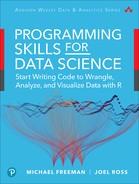
If you see a plus sign (
+) in the terminal as opposed to the typical greater than symbol (>)—as in Figure 5.4—you have probably forgotten to close a quotation mark. If you find yourself in this situation, you can press theesckey to cancel the line of code and start over. This will also work if you forget to close a set of parentheses (()) or brackets ([]).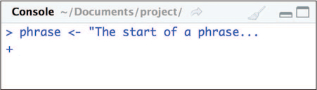
Figure 5.4 An unclosed statement in the RStudio console: press the esckey to cancel the statement and return to the command prompt.Logical: Logical (boolean) data types store “yes-or-no” data. A logical value can be one of two values:
TRUEorFALSE. Importantly, these are not the strings"TRUE"or"FALSE"; logical values are a different type! If you prefer, you can use the shorthandTorFin lieu ofTRUEandFALSEin variable assignment.Fun Fact
Logical values are called “booleans” after mathematician and logician George Boole.
Logical values are most commonly produced by applying a relational operator (also called a comparison operator) to some other data. Comparison operators are used to compare values and include
<(less than),>(greater than),<=(less than or equal),>=(greater than or equal),==(equal), and!=(not equal). Here are a few examples:# Store values in variables (number of strings on an instrument) num_guitar_strings <- 6 num_mandolin_strings <- 8 # Compare the number of strings on each instrument num_guitar_strings > num_mandolin_strings # returns logical value FALSE num_guitar_strings != num_mandolin_strings # returns logical value TRUE # Equivalently, you can compare values that are not stored in variables 6 == 8 # returns logical value FALSE # Use relational operators to compare two strings "mandolin" > "guitar" # returns TRUE (m comes after g alphabetically)
If you want to write a more complex logical expression (i.e., for when something is true and something else is false), you can do so using logical operators (also called boolean operators). These include
&(and),|(or), and!(not).# Store the number of instrument players in a hypothetical band num_guitar_players <- 3 num_mandolin_players <- 2 # Calculate the number of band members total_band_members <- num_guitar_players + num_mandolin_players # 5 # Calculate the total number of strings in the band # Shown on two lines for readability, which is still valid R code total_strings <- num_guitar_players * num_guitar_strings + num_mandolin_strings * num_mandolin_players # 34 # Are there fewer than 30 total strings AND fewer than 6 band members? total_strings < 30 & total_band_members < 6 # FALSE # Are there fewer than 30 total strings OR fewer than 6 band members? total_strings < 30 | total_band_members < 6 # TRUE # Are there 3 guitar players AND NOT 3 mandolin players? # Each expression is wrapped in parentheses for increased clarity (num_guitar_players == 3) & ! (num_mandolin_players == 3) # TRUE
It’s easy to write complex—even overly complex—expressions with logical operators. If you find yourself getting lost in your logic, we recommend rethinking your question to see if there is a simpler way to express it!
Integer: Integer (whole-number) values are technically a different data type than numeric values because of how they are stored and manipulated by the
Rinterpreter. This is something that you will rarely encounter, but it’s good to know that you can specify that a number is of the integer type rather than the general numeric type by placing a capitalL(for “long integer”) after a value in variable assignment (my_integer <- 10L). You will rarely do this intentionally, but this is helpful for answering the question, Why is there an L after my number…?Complex: Complex (imaginary) numbers have their own data storage type in
R, and are created by placing aniafter the number:complex_variable <- 2i. We will not be using complex numbers in this book, as they rarely are important for data science.
5.5 Getting Help
As with any programming language, you will inevitably run into problems, confusing situations, or just general questions when working in R. Here are a few ways to start getting help.
Read the error messages: If there is an issue with the way you have written or executed your code,
Rwill often print out an error message in your console (in red in RStudio). Do your best to decipher the message—read it carefully, and think about what is meant by each word in the message—or you can put that message directly into Google to search for more information. You will soon get the hang of interpreting these messages if you put the time into trying to understand them. For example, Figure 5.5 shows the result of accidentally mistyping a variable name. In that error message,Rindicated that the objectctywas not found. This makes sense, because the code never defined a variablecty(the variable was calledcity).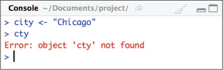
Figure 5.5 RStudio showing an error message due to a typo (there is no variable cty). Google: When you’re trying to figure out how to do something, it should come as no surprise that search engines such as Google are often the best resource. Try searching for queries like
"how to DO_THING in R". More frequently than not, your question will lead you to a Q&A forum called StackOverflow (discussed next), which is a great place to find potential answers.StackOverflow: StackOverflow is an amazing Q&A forum for asking/answering programming questions. Indeed, most basic questions have already been asked and answered there. However, don’t hesitate to post your own questions to StackOverflow. Be sure to hone in on the specific question you’re trying to answer, and provide error messages and sample code. You will often find that by the time you can articulate the question clearly enough to post it, you will have figured out your problem anyway.
Tip
There is a classical method of fixing errors called rubber duck debugging, which involves trying to explain your code/problem to an inanimate object (talking to pets works too). You will usually be able to fix the problem if you just step back and think about how you would explain it to someone else!
Built-in documentation:
R’s documentation is actually pretty good. Functions and behaviors are all described in the same format, and often contain helpful examples. To search the documentation withinR(or in RStudio), type a question mark (?) followed by the function name you’re using (e.g,?sum). You can perform a broader search of available documentation by typing two questions marks (??) followed by your search term (e.g.,??sum).You can also look up help by using the
help()function (e.g.,help(print)will look up information on theprint()function, just as?printdoes). There is also anexample()function you can call to see examples of a function in action (e.g.,example(print)). This will be more applicable starting in Chapter 6.In addition, RDocumentation.org3 has a lovely searchable and readable interface to the
Rdocumentation.RStudio Community: RStudio recently launched an online community4 for
Rusers. The intention is to build a more positive online community for getting programming help withRand engaging with the open source community using the software.
3RDocumentation.org: https://www.rdocumentation.org
4RStudio Community: https://community.rstudio.com
5.5.1 Learning to Learn R
This chapter has demonstrated the basics of the R programming language, and further features are detailed through the rest of the book. However, it’s not possible to cover all features of a particular programming language—not to mention its surrounding ecosystem, such as the other frameworks used in data science—especially in a way that is accessible to those who are just getting started. While we will cover all of the material that you need to get started and ask questions of data using code, you will most certainly encounter problems in the future that aren’t discussed in this text. Doing data science will require continuously learning new skills and techniques that are more advanced, more specific to your problem, or simply hadn’t been invented when this book was written!
Luckily, you’re not alone in this process! There is a huge number of resources that you can use to help you learn R or any other topic in programming or data science. This section provides an overview and examples of the types of resources you might use.
Books: Many excellent text resources are available both in print and for free online. Books can provide a comprehensive overview of a topic, usually with a large number of examples and links to even more resources. We typically recommend them for beginners, as they help to cover all of the myriad steps involved in programming and their extensive examples help inform good programming habits. Free online books are easily accessible (and allow you to copy-and-paste code examples), but physical print can provide a useful point of reference (and typing out examples is a great way to practice).
For learning
Rin particular, R for Data Science5 is one of the best free online textbooks, covering the programming language through the lens of thetidyversecollection of packages (which are used in this book as well). Excellent print books include R for Everyone6 and The Art of R Programming.75Wickham, H., & Grolemund, G. (2016). R for Data Science. O’Reilly Media, Inc. http://r4ds.had.co.nz
6Lander, J. P. (2017). R for Everyone: Advanced Analytics and Graphics (2nd ed.). Boston, MA: Addison-Wesley.
7Matloff, N. (2011). The Art of R Programming: A Tour of Statistical Software Design. San Francisco, CA: No Starch Press.
Tutorials and videos: The internet is also host to a large number of more informal explanations of programming concepts. These range from mini-books (such as the opinionated but clear introduction aRrgh: a newcomer’s (angry) guide to R8), to tutorial series (such as those provided by R Tutor9 or Quick-R10), to focused articles and guides (e.g., posts on R-bloggers11), to particularly informative StackOverflow responses. These smaller guides are particularly useful when you’re trying to answer a specific question or clarify a single concept—when you want to know how to do one thing, not necessarily understand the entire language. In addition, many people have created and shared online video tutorials (such as Pearson’s LiveLessons12), often in support of a course or textbook. Video code blogging is even more common in other programming languages such as JavaScript. Video demonstrations are great at showing you how to actually use a programming concept in practice—you can see all the steps that go into a program (though there is no substitute for doing it yourself).
8aRrgh: a newcomer’s (angry) guide to R: http://arrgh.tim-smith.us
9R Tutor: http://www.r-tutor.com/; start with the introduction at http://www.r-tutor.com/r-introduction
10Quick-R: https://www.statmethods.net/index.html; be sure and follow the hyperlinks.
11R-Bloggers: https://www.r-bloggers.com
12LiveLessons video tutorials: https://www.youtube.com/user/livelessons
Because such guides can be created and hosted by anyone, the quality and accuracy may vary. It’s always a good idea to confirm your understanding of a concept with multiple sources (do multiple tutorials agree?), with your own experience (does the solution actually work for your code?), and your own intuition (does that seem like a sensible explanation?). In general, we encourage you to start with more popular or official guides, as they are more likely to encourage best practices.
Interactive tutorials and courses: The best way to learn any skill is by doing it, and there are multiple interactive websites that will let you learn and practice programming right in your web browser. These are great for seeing topics in action or for experimenting with different options (though it is simple enough to experiment inside of RStudio—an approach taken by the swirl13 package).
13swirl interactive tutorial: http://swirlstats.com
The most popular set of interactive tutorials for
Rprogramming are provided by DataCamp14 and are presented as online courses (a sequence of explanations and exercises that you can learn to use a skill) on different topics. DataCamp tutorials provide videos and interactive tutorials for a wide range of different data science topics. While most of the introductory courses (e.g., Introduction to R15) are free, more advanced courses require you to sign up and pay for the service. Nevertheless, even at the free level, this is an effective set of resources for picking up new skills.14DataCamp: https://www.datacamp.com/home
15DataCamp: Introduction to R: https://www.datacamp.com/courses/free-introduction-to-r
In addition to these informal interactive courses, it is possible to find more formal online courses in
Rand data science through massive open online course (MOOC) services such as Coursera16 or Udacity.17 For example, the Data Science at Scale18 course from the University of Washington offers a deep introduction to data science (though it assumes some programming experience, so it may be more appropriate for after you’ve finished this book!). Note that these online courses almost always require a paid fee, though you can sometimes earn university credit or certifications from them.16Coursera: https://www.coursera.org
17Udacity: https://www.udacity.com
18Data Science at Scale: online course from the University of Washington: https://www.coursera.org/specializations/data-science
Documentation: One of the best places to start out when learning a programming concept is the official documentation. In addition to the base
Rdocumentation described in the previous section, many system creators will produce useful “getting started” guides and references—called “vignettes” in theRcommunity—that you can use (to encourage adoption of their tool). For example, thedplyrpackage (described in great detail in Chapter 11) has an official “getting started” summary on its homepage19 as well as a complete reference.20 Further detail on a package may also often be found linked from that package’s homepage on GitHub (where the documentation can be kept under version control); checking the GitHub page for a package or library is often an effective way to gain more information about it. Additionally, manyRpackages host their documentation in.pdfformat on CRAN’s website; to learn to use a package, you will need to read its explanation carefully and try out its examples!19
dplyrhomepage: https://dplyr.tidyverse.org20
dplyrreference: https://dplyr.tidyverse.org/reference/index.htmlCommunity resources: As
Ris an open source language, many of theRresources described here are created by the community of programmers—and this community can be one of the best resources for learning to program. In addition to community-generated tutorials and answers to questions, in-person meet-ups can be an excellent source for getting help (particularly in larger urban areas). Check whether your city or town has a local “useR” group that may host events or training sessions.
This section lists only a few of the many, many resources for learning R. You can find many more online resources on similar topics by searching for “TOPIC tutorial” or “how to DO_SOMETHING in R.” You may also find other compilations of resources. For example, RStudio has put together a list21 of its recommended tutorials and resources.
21RStudio: Online Learning resource collection: https://www.rstudio.com/online-learning/
In the end, remember that the best way to learn about anything—whether about programming or from a set of data—is to ask questions. For practice writing code in R and familiarizing yourself with RStudio, see the set of accompanying book exercises.22
22Introductory R exercises: https://github.com/programming-for-data-science/chapter-05-exercises