In C++, any function can call another function. A function can even call itself! When a function calls itself, it is making a recursive call. The word recursive means “having the characteristic of coming up again, or repeating.” In this case, a function call is being repeated by the function itself. Recursion is a powerful technique that can be used in place of iteration (looping).

Recursive solutions are generally less efficient than iterative solutions to the same problem. However, some problems lend themselves to simple, elegant, recursive solutions and are exceedingly cumbersome to solve iteratively. Some programming languages, such as early versions of Fortran, Basic, and COBOL, do not allow recursion. Other languages are especially oriented to recursive algorithms—LISP is one of these. C++ lets us take our choice: We can implement both iterative and recursive algorithms.

Our examples are broken into two groups: problems that use only simple variables and problems that use structured variables. If you are studying recursion before reading Chapters 11-16 on structured data types, then cover only the first set of examples and leave the rest until you have completed the chapters on structured data types.

18.1 What Is Recursion?

You may have seen a set of gaily painted Russian dolls that fit inside one another. Inside the first doll is a smaller doll, inside of which is an even smaller doll, inside of which is yet a smaller doll, and so on. A recursive algorithm is like such a set of Russian dolls. It reproduces itself with smaller and smaller examples of itself until a solution is found—that is, until there are no more dolls. The recursive algorithm is implemented by using a function that makes recursive calls to itself.

In Chapter 8, we wrote a function named Power that calculates the result of raising an integer to a positive power. If X is an integer and N is a positive integer, the formula for X^N is

We could also write this formula as

or even as

In fact, we can write the formula most concisely as

X^N = X × X^N-1

This definition of X^N is a classic recursive definition—that is, a definition given in terms of a smaller version of itself.

X^N is defined in terms of multiplying X times X^N-1. How is X^N-1 defined? Why, as X × X^N-2, of course! And X^N-2 is X × X^N-3; X^N-3 is X × X^N-4; and so on. In this example, “in terms of smaller versions of itself” means that the exponent is decremented each time.

When does the process stop? When we have reached a case for which we know the answer without resorting to a recursive definition. In this example, it is the case where N equals 1: X¹ is X. The case (or cases) for which an answer is explicitly known is called the base case. The case for which the solution is expressed in terms of a smaller version of itself is called the recursive or general case. A recursive algorithm is an algorithm that expresses the solution in terms of a call to itself, a recursive call. A recursive algorithm must terminate; that is, it must have a base case.

The following program shows a recursive version of the Power function with the base case and the recursive call marked. The function is embedded in a program that reads in a number and an exponent and prints the result.

Each recursive call to Power can be thought of as creating a completely new copy of the function, each with its own copies of the parameters x and n. The value of x remains the same for each version of Power, but the value of n decreases by 1 for each call until it becomes 1.

Let's trace the execution of this recursive function, with number equal to 2 and exponent equal to 3. We use a new format to trace recursive routines: We number the calls and then discuss what is happening in paragraph form.

Call 1: Power is called by main, with number equal to 2 and exponent equal to 3. Within Power, the parameters x and n are initialized to 2 and 3, respectively. Because n is not equal to 1, Power is called recursively with x and n - 1 as arguments. Execution of Call 1 pauses until an answer is sent back from this recursive call.

Call 2: x is equal to 2 and n is equal to 2. Because n is not equal to 1, the function Power is called again, this time with x and n - 1 as arguments. Execution of Call 2 pauses until an answer is sent back from this recursive call.

Call 3: x is equal to 2 and n is equal to 1. Because n equals 1, the value of x is to be returned. This call to the function has finished executing, and the function return value (which is 2) is passed back to the place in the statement from which the call was made.

Call 2: This call to the function can now complete the statement that contained the recursive call because the recursive call has returned. Call 3's return value (which is 2) is multiplied by x. This call to the function has finished executing, and the function return value (which is 4) is passed back to the place in the statement from which the call was made.

Call 1: This call to the function can now complete the statement that contained the recursive call because the recursive call has returned. Call 2's return value (which is 4) is multiplied by x. This call to the function has finished executing, and the function return value (which is 8) is passed back to the place in the statement from which the call was made. Because the first call (the nonrecursive call in main) has now completed, this is the final value of the function Power.

This trace is summarized in FIGURE 18.1. Each box represents a call to the Power function. The values for the parameters for that call are shown in each box.

Figure 18.1 Execution of Power(2,3)

What happens if there is no base case? We have infinite recursion, the recursive equivalent of an infinite loop. For example, if the condition

if (n == 1)

were omitted, Power would be called over and over again. Infinite recursion also occurs if Power is called with n less than or equal to 0.

In actuality, recursive calls cannot go on forever. Here's the reason. When a function is called, either recursively or nonrecursively, the computer system creates temporary storage for the parameters and the function's (automatic) local variables. This temporary storage is a region of memory called the run-time stack. When the function returns, its parameters and local variables are released from the run-time stack. With infinite recursion, the recursive function calls never return. Each time the function calls itself, a little more of the run-time stack is used to store the new copies of the variables. Eventually, all the memory space on the stack is used. At that point, the program crashes with an error message such as “Runtime stack overflow” (or the computer may simply hang).

18.2 Recursive Algorithms with Simple Variables

Let's look at another example: calculating a factorial. The factorial of a number N (written N!) is N multiplied by N - 1, N - 2, N - 3, and so on. Another way of expressing factorial is

N! = N × (N - 1)!

This expression looks like a recursive definition. (N - 1)! is a smaller instance of N!—that is, it takes one less multiplication to calculate (N - 1)! than it does to calculate N! If we can find a base case, we can write a recursive algorithm. Fortunately, we don't have to look too far: 0! is defined in mathematics to be 1.

Factorial (In: n)

IF n is 0
    Return 1
  ELSE
    Return n * Factorial (n-1)

This algorithm can be coded directly as follows:

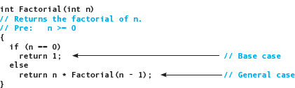
Let's trace this function with an original n of 4.

Call 1: n is 4. Because n is not 0, the else branch is taken. The Return statement cannot be completed until the recursive call to Factorial with n - 1 as the argument has been completed.

Call 2: n is 3. Because n is not 0, the else branch is taken. The Return statement cannot be completed until the recursive call to Factorial with n - 1 as the argument has been completed.

Call 3: n is 2. Because n is not 0, the else branch is taken. The Return statement cannot be completed until the recursive call to Factorial with n - 1 as the argument has been completed.

Call 4: n is 1. Because n is not 0, the else branch is taken. The Return statement cannot be completed until the recursive call to Factorial with n - 1 as the argument has been completed.

Call 5: n is 0. Because n equals 0, this call to the function returns, sending back 1 as the result.

Call 4: The Return statement in this copy can now be completed. The value to be returned is n (which is 1) times 1. This call to the function returns, sending back 1 as the result.

Call 3: The Return statement in this copy can now be completed. The value to be returned is n (which is 2) times 1. This call to the function returns, sending back 2 as the result.

Call 2: The Return statement in this copy can now be completed. The value to be returned is n (which is 3) times 2. This call to the function returns, sending back 6 as the result.

Call 1: The Return statement in this copy can now be completed. The value to be returned is n (which is 4) times 6. This call to the function returns, sending back 24 as the result. Because this is the last of the calls to Factorial, the recursive process is over. The value 24 is returned as the final value of the call to Factorial with an argument of 4.

FIGURE 18.2 summarizes the execution of the Factorial function with an argument of 4.

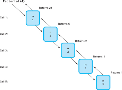
Figure 18.2 Execution of Factorial(4)

Let's organize what we have done in these two solutions into an outline for writing recursive algorithms:

1. Understand the problem. (We threw this one in for good measure; it is always the first step.)

2. Determine the base case(s).

3. Determine the recursive case(s).

We have used the factorial and the power algorithms to demonstrate recursion because they are easy to visualize. In practice, one would never want to calculate either of these functions using the recursive solution. In both cases, the iterative solutions are simpler and much more efficient because starting a new iteration of a loop is a faster operation than calling a function. Let's compare the code for the iterative and recursive versions of the factorial problem.

Iterative Solution                     Recursive Solution
int Factorial (int n)                  int Factorial (int n)
{                                      {
  int factor;                             if (n == 0)
  int count;                                return 1;
                                          else
  factor = 1;                               return n * Factorial (n-1);
  for (count = 2; count <= n;          }
       count++)
    factor = factor * count;
  return factor;
}

The iterative version has two local variables, whereas the recursive version has none. There are usually fewer local variables in a recursive routine than in an iterative routine. Also, the iterative version always has a loop, whereas the recursive version always has a selection statement—either an If or a Switch. A branching structure is the main control structure in a recursive routine. A looping structure is the main control structure in an iterative routine.

In the next section, we examine a more complicated problem—one in which the recursive solution is not immediately apparent.

18.3 Towers of Hanoi

One of your first toys may have been three pegs with colored circles of different diameters. If so, you probably spent countless hours moving the circles from one peg to another. If we put some constraints on how the circles or discs can be moved, we have an adult game called the Towers of Hanoi. When the game begins, all the circles are on the first peg in order by size, with the smallest on the top. The object of the game is to move the circles, one at a time, to the third peg. The catch is that a circle cannot be placed on top of one that is smaller in diameter. The middle peg can be used as an auxiliary peg, but it must be empty at the beginning and at the end of the game.

To get a feel for how this might be done, let's look at some sketches of what the configuration must be at certain points if a solution is possible. We use four circles or discs. Here is the beginning configuration:

To move the largest circle (circle 4) to peg 3, we must move the three smaller circles to peg 2. Then circle 4 can be moved into its final place:

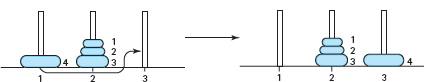
Let's assume we can do this. Now, to move the next largest circle (circle 3) into place, we must move the two circles on top of it onto an auxiliary peg (peg 1 in this case):

To get circle 2 into place, we must move circle 1 to another peg, freeing circle 2 to be moved to its place on peg 3:

The last circle (circle 1) can now be moved into its final place, and we are finished:

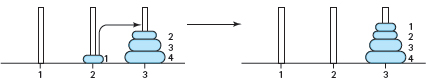
Notice that to free circle 4, we had to move three circles to another peg. To free circle 3, we had to move two circles to another peg. To free circle 2, we had to move one circle to another peg. This sounds like a recursive algorithm: To free the nth circle, we have to move n - 1 circles. Each stage can be thought of as beginning again with three pegs, but with one less circle each time. Let's see if we can summarize this process, using n instead of an actual number.

Get n Circles Moved from Peg 1 to Peg 3

Get n-1 circles moved from peg1 to peg2
Move nth circle from peg1 to peg3
Get n-1 circles moved from peg2 to peg3

This algorithm certainly sounds simple; surely there must be more. But this really is all there is to it.

Let's write a recursive function that implements this algorithm. We can't actually move discs, of course, but we can print out a message to do so. Notice that the beginning peg, the ending peg, and the auxiliary peg keep changing during the algorithm. To make the algorithm easier to follow, we call the pegs beginPeg, endPeg, and auxPeg. These three pegs, along with the number of circles on the beginning peg, are the parameters of the function.

We have the recursive or general case, but what about a base case? How do we know when to stop the recursive process? The clue is in the statement “Get n circles moved.” If we don't have any circles to move, we don't have anything to do. We are finished with that stage. Therefore, when the number of circles equals 0, we do nothing (that is, we simply return).

void DoTowers(
   int circleCount,     // Number of circles to move
   int beginPeg,        // Peg containing circles to move
   int auxPeg,          // Peg holding circles temporarily
   int endPeg)          // Peg receiving circles being moved
{
  if (circleCount > 0)
  {
    // Move n - 1 circles from beginning peg to auxiliary peg
    DoTowers(circleCount - 1, beginPeg, endPeg, auxPeg);
    cout << “Move circle from peg “ << beginPeg
         << “ to peg “ << endPeg << endl;
    // Move n - 1 circles from auxiliary peg to ending peg
    DoTowers(circleCount - 1, auxPeg, beginPeg, endPeg);
  }
}

It's hard to believe that such a simple algorithm actually works, but we'll prove it to you. Following is a driver program that calls the DoTowers function. Output statements have been added so you can see the values of the arguments with each recursive call. Because there are two recursive calls within the function, we have indicated which recursive statement issued the call.

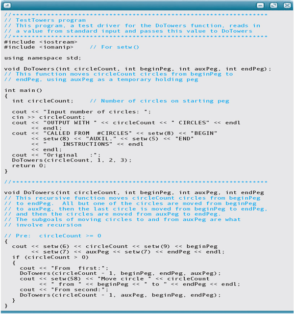
The output from a run with three circles follows. “Original” means that the parameters listed beside it are from the nonrecursive call, which is the first call to DoTowers. “From first” means that the parameters listed are for a call issued from the first recursive statement. “From second” means that the parameters listed are for a call issued from the second recursive statement. Notice that a call cannot be issued from the second recursive statement until the preceding call from the first recursive statement has completed execution.

18.4 Recursive Algorithms with Structured Variables

In our definition of a recursive algorithm, we said there were two cases: the recursive or general case, and the base case for which an answer can be expressed nonrecursively. In the general case for all our algorithms so far, an argument was expressed in terms of a smaller value each time. When structured variables are used, the recursive case is often given in terms of a smaller structure rather than a smaller value; the base case occurs when there are no values left to process in the structure.

Let's examine a recursive algorithm for printing the contents of a one-dimensional array of n elements to show what this means.

Print Array

  IF more elements
    Print the value of the first element
    Print the array of n-1 elements

The recursive case is to print the values in an array that is one element “smaller”; that is, the size of the array decreases by 1 with each recursive call. The base case is when the size of the array becomes 0—that is, when there are no more elements to print.

Our arguments must include the index of the first element (the one to be printed). How do we know when there are no more elements to print (that is, when the size of the array to be printed is 0)? We know we have printed the last element in the array when the index of the next element to be printed is beyond the index of the last element in the array. Therefore, the index of the last array element must be passed as an argument. We call these indexes first and last. When first is greater than last, we are finished. The name of the array is data.

void Print(const int data[], int first, int last)
// This function prints the values in data from data[first]
// through data[last]
{
  if (first <= last)
  {                                              // Recursive case
    cout << data[first] << endl;
    Print(data, first + 1, last);
  }
    // Empty else-clause is the base case
}

Here is a code walk-through of the function call

Print(data, 0, 4);

using the pictured array:

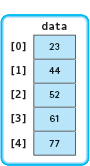
Call 1: first is 0 and last is 4. Because first is less than last, the value in data[first] (which is 23) is printed. Execution of this call pauses while the array from first + 1 through last is printed.

Call 2: first is 1 and last is 4. Because first is less than last, the value in data[first] (which is 44) is printed. Execution of this call pauses while the array from first + 1 through last is printed.

Call 3: first is 2 and last is 4. Because first is less than last, the value in data[first] (which is 52) is printed. Execution of this call pauses while the array from first + 1 through last is printed.

Call 4: first is 3 and last is 4. Because first is less than last, the value in data[first] (which is 61) is printed. Execution of this call pauses while the array from first + 1 through last is printed.

Call 5: first is 4 and last is 4. Because first is equal to last, the value in data[first] (which is 77) is printed. Execution of this call pauses while the array from first + 1 through last is printed.

Call 6: first is 5 and last is 4. Because first is greater than last, the execution of this call is complete. Control returns to the preceding call.

Call 5: Execution of this call is complete. Control returns to the preceding call.

Calls 4, 3, 2, and 1: Each execution is completed in turn, and control returns to the preceding call.

Notice that once the deepest call (the call with the highest number) was reached, each of the calls before it returned without doing anything. When no statements are executed after the return from the recursive call to the function, the recursion is known as tail recursion. Tail recursion often indicates that the problem could be solved more easily using iteration. We used the array example because it made the recursive process easy to visualize; in practice, an array should be printed iteratively.

FIGURE 18.3 shows the execution of the Print function with the values of the parameters for each call. Notice that the array gets smaller with each recursive call (data[first] through data[last]). If we want to print the array elements in reverse order recursively, all we have to do is interchange the two statements within the If statement.

Figure 18.3 Execution of Print(data, 0, 4)

18.5 Recursion Using Pointer Variables

The recursive algorithm for printing a one-dimensional array could have been implemented much more easily using iteration. Now we look at two algorithms that cannot be handled more easily with iteration: printing a linked list in reverse order and creating a duplicate copy of a linked list. We call the external pointer to the list listPtr.

Printing a Dynamic Linked List in Reverse Order

Printing a linked list in order from first to last is easy. We set a running pointer (ptr) equal to listPtr and cycle through the list until ptr becomes NULL.

Print List (In: listPtr)

Set ptr to listPtr
  WHILE ptr is not NULL
    Print ptr->component
    Set ptr to ptr->link

To print the list in reverse order, we must print the value in the last node first, then the value in the next-to-last node, and so on. Another way of expressing this process is to say that we do not print a value until the values in all the nodes following it have been printed. We might visualize the process as the first node's turning to its neighbor and saying, “Tell me when you have printed your value. Then I'll print my value.” The second node says to its neighbor, “Tell me when you have printed your value. Then I'll print mine.” That node, in turn, says the same to its neighbor, and so on, until there is nothing to print.

Because the number of neighbors gets smaller and smaller, we seem to have the makings of a recursive solution. The end of the list is reached when the running pointer is NULL. When that happens, the last node can print its value and send the message back to the one before it. That node can then print its value and send the message back to the one before it, and so on.

RevPrint (In: listPtr)

IF listPtr is not NULL
   RevPrint rest of nodes in list
   Print current node in list

This algorithm can be coded directly as the following function:

void RevPrint(NodePtr listPtr)
// Pre:  listPtr points to a list node or is NULL
// Post: If listPtr is not NULL, all nodes after listPtr have
//       been printed followed by the contents of listPtr;
//       else no action has been taken.
{
  if (listPtr != NULL)
  {
    RevPrint(listPtr->link);                      // Recursive call
    cout << listPtr->component << endl;
  }
  // Empty else-clause is the base case
}

This algorithm seems complex enough to warrant a code walk-through. We use the following list:

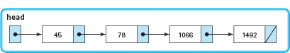
Call 1: listPtr points to the node containing 45 and is not NULL. Execution of this call pauses until the recursive call with the argument listPtr->link has been completed.

Call 2: listPtr points to the node containing 78 and is not NULL. Execution of this call pauses until the recursive call with the argument listPtr->link has been completed.

Call 3: listPtr points to the node containing 1066 and is not NULL. Execution of this call pauses until the recursive call with the argument listPtr->link has been completed.

Call 4: listPtr points to the node containing 1492 and is not NULL. Execution of this call pauses until the recursive call with the argument listPtr->link has been completed.

Call 5: listPtr is NULL. Execution of this call is complete. Control returns to the preceding call.

Call 4: listPtr->component (which is 1492) is printed. Execution of this call is complete. Control returns to the preceding call.

Call 3: listPtr->component (which is 1066) is printed. Execution of this call is complete. Control returns to the preceding call.

Call 2: listPtr->component (which is 78) is printed. Execution of this call is complete. Control returns to the preceding call.

Call 1: listPtr->component (which is 45) is printed. Execution of this call is complete. Because this is the nonrecursive call, execution continues with the statement immediately following RevPrint(listPtr).

FIGURE 18.5 shows the execution of the RevPrint function. The parameters are pointers (memory addresses), so we use? 45 to mean the pointer to the node whose component is 45.

Figure 18.5 Execution of RevPrint

Copying a Dynamic Linked List

When working with linked lists, we sometimes need to create a duplicate copy (sometimes called a clone) of a linked list. For example, in Chapter 14, we wrote a copy-constructor for the List class. This copy-constructor creates a new class object that is a copy of another class object, including its dynamic linked list.

Suppose that we want to write a value-returning function that receives the external pointer to a linked list (listPtr), makes a clone of the linked list, and returns the external pointer to the new list as the function value. A typical call to the function would be the following:

NodePtr listPtr;
NodePtr newListPtr;
  .
  .
  .
newListPtr = PtrToCopy(listPtr);

Using iteration to copy a linked list is rather complicated. The following algorithm is essentially the same as the one used in the List copy-constructor.

PtrToCopy (In: listPtr) // Iterative algorithm Out: Function value

IF listPtr is NULL
   Return NULL
// Copy first node
Set fromPtr = listPtr
Set copyPtr = new NodeType
Set copyPtr->component = fromPtr->component
// Copy remaining nodes
Set toPtr = copyPtr
Set fromPtr = fromPtr->link
WHILE fromPtr is not NULL
   Set toPtr->link = new NodeType
   Set toPtr = toPtr->link
   Set toPtr->component = fromPtr->component
   Set fromPtr = fromPtr->link
Set toPtr->link = NULL
Return copyPtr

A recursive solution to this problem is far simpler, but it requires us to think recursively. To copy the first node of the original list, we can allocate a new dynamic node and copy the component value from the original node into the new node. However, we cannot yet fill in the link member of the new node: We must wait until we have copied the second node, so that we can store its address into the link member of the first node. Likewise, the copying of the second node cannot complete until we have finished copying the third node. Eventually, we copy the last node of the original list and set the link member of the copy node to NULL. At this point, the last node returns its own address to the next-to-last node, which stores the address into its link member. The next-to-last node returns its own address to the node before it, and so forth. The process is complete when the first node returns its address to the first (nonrecursive) call, yielding an external pointer to the new linked list.

PtrToCopy (In: fromPtr) // Recursive algorithm Out: Function value

IF fromPtr is NULL
   Return NULL
 ELSE
   Set toPtr = new NodeType
   Set toPtr->component = fromPtr->component
   Set toPtr->link = PtrToCopy(fromPtr->link)
   Return toPtr

Like the solution to the Towers of Hanoi problem, this scheme looks too simple—yet it is the full algorithm. Because the argument that is passed to each recursive call is fromPtr-> link, the number of nodes left in the original list becomes smaller with each call. The base case occurs when the pointer into the original list becomes NULL. Following is the C++ function that implements this algorithm.

NodePtr PtrToCopy(NodePtr fromPtr)
// Pre:  fromPtr points to a list node or NULL
// Post: If fromPtr is not NULL, a copy of the entire sublist
//         starting with *fromPtr is on the free store and
//         function value is the pointer to front of this sublist
//       else
//          Return value is NULL
{
  NodePtr toPtr;      // Pointer to newly created node
  if (fromPtr == NULL)
    return NULL;                     // Base case
  else
  {                                  // Recursive case
    toPtr = new NodeType;
    toPtr->component = fromPtr->component;
    toPtr->link = PtrToCopy(fromPtr->link);
    return toPtr;
  }
}

Let's perform a code walk-through of the function call

newListPtr = PtrToCopy(listPtr);

using the following list:

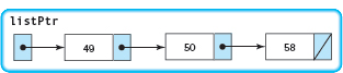
Call 1: fromPtr points to the node containing 49 and is not NULL. A new node is allocated and its component value is set to 49.

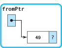
Execution of this call pauses until the recursive call with the argument fromPtr->link has been completed.

Call 2: fromPtr points to the node containing 50 and is not NULL. A new node is allocated and its component value is set to 50.

Execution of this call pauses until the recursive call with the argument fromPtr->link has been completed.

Call 3: fromPtr points to the node containing 58 and is not NULL. A new node is allocated and its component value is set to 58.

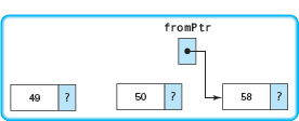
Execution of this call pauses until the recursive call with the argument fromPtr->link has been completed.

Call 4: fromPtr is NULL. The list is unchanged.

Execution of this call is complete. NULL is returned as the function value to the preceding call.

Call 3: Execution of this call resumes by assigning the returned function value (NULL) to toPtr->link.

Execution of this call is complete. The value of toPtr is returned to the preceding call.

Call 2: Execution of this call resumes by assigning the returned function value (the address of the third node) to toPtr->link.

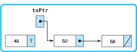
Execution of this call is complete. The value of toPtr is returned to the preceding call.

Call 1: Execution of this call resumes by assigning the returned function value (the address of the second node) to toPtr->link.

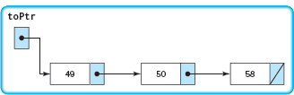
Execution of this call is complete. Because this is the nonrecursive call, the value of toPtr is returned to the assignment statement containing the original call. The variable newListPtr now points to a copy of the original list.

18.6 Recursion or Iteration?

Recursion and iteration are alternative ways of expressing repetition in a program. When iterative control structures are used, processes are made to repeat by embedding code in a looping structure such as a While, For, or Do-While. In recursion, a process is made to repeat by having a function call itself; a selection statement is used to control the repeated calls.

Which is the better approach—recursion or iteration? There is no simple answer to this question. The choice usually depends on two issues: efficiency and the nature of the problem being solved.

Historically, the quest for efficiency, in terms of both execution speed and memory usage, has favored iteration over recursion. Each time a recursive call is made, the system must allocate stack space for all parameters and (automatic) local variables. The overhead involved in any function call is time-consuming. On early, slow computers with limited memory capacity, recursive algorithms were visibly—sometimes painfully—slower than the iterative versions. By contrast, on modern, fast computers, the overhead of recursion is often so small that the increase in computation time is almost unnoticeable to the user. Except in cases where efficiency is absolutely critical, then, the choice between recursion and iteration more often depends on the second issue—the nature of the problem being solved.

Consider the factorial and power algorithms discussed earlier in this chapter. In both cases, iterative solutions were obvious and easy to devise. We imposed recursive solutions on these problems simply to demonstrate how recursion works. As a rule of thumb, if an iterative solution is more obvious or easier to understand, use it; it will be more efficient. In some other problems, the recursive solution is more obvious or easier to devise, such as in the Towers of Hanoi problem. (It turns out that the Towers of Hanoi problem is surprisingly difficult to solve using iteration.) Computer science students should be aware of the power of recursion. If the definition of a problem is inherently recursive, then a recursive solution should certainly be considered.
 

Problem-Solving Case Study

Quicksort

PROBLEM: Throughout the last half of this book, we have worked with lists of items, both sorted and unsorted. At the logical level, sorting algorithms take an unsorted list and convert it into a sorted list. At the implementation level, sorting algorithms take an array and reorganize the data into some sort of order. We have used the straight selection algorithm to sort a list of numbers, and we have inserted entries into a list ordered by time. In this case study, we will create a function template that implements the Quicksort algorithm.

DISCUSSION: The Quicksort algorithm, which was developed by C. A. R. (Tony) Hoare, is based on the idea that it is faster and easier to sort two small lists than one larger one. The name comes from the fact that, in general, a Quicksort can sort a list of data elements quite rapidly. The basic strategy of this sort is to “divide and conquer.”

If you were given a large stack of final exams to sort by name, you might use the following approach: Pick a splitting value—say, L—and divide the stack of tests into two piles, A-L and M-Z. (Note that the two piles do not necessarily contain the same number of tests.) Then take the first pile and subdivide it into two piles, A-F and G-L. The A-F pile can be further broken down into A-C and D-F. This division process goes on until the piles are small enough to be easily sorted by hand. The same process is applied to the M-Z pile. Eventually all of the small sorted piles can be stacked one on top of the other to produce a sorted set of tests. (See FIGURE 18.6.)

This strategy is based on recursion—on each attempt to sort the stack of tests, the stack is divided and then the same approach is used to sort each of the smaller stacks (a smaller case). This process goes on until the small stacks do not need to be further divided (the base case). The parameter list of the Quicksort algorithm specifies the part of the list that is currently being processed. Notice that we are sorting the list items stored in the array—not an abstract list about whose implementation we know nothing. To make this distinction clear, we call the array data rather than list.

Figure 18.6 Ordering a List Using the Quicksort Algorithm

IF there is more than one item in data[first]..data[last]
    Select splitVal
    Split the data so that
      data[first]..data[splitPoint-1] <= splitVal
      data[splitPoint] = splitVal
      data[splitPoint+1]..data[last] > splitVal
    Quicksort the left half
    Quicksort the right half

How do we select splitVal? One simple solution is to use whatever value is in data[first] as the splitting value. Let's look at an example using data[first] as splitVal.

After the call to Split, all of the items less than or equal to splitVal are on the left side of the data and all of those items greater than splitVal are on the right side of the data.

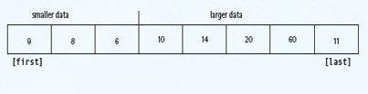
The two “halves” meet at splitPoint, the index of the last item that is less than or equal to splitVal. Note that we don't know the value of splitPoint until the splitting process is complete. We can then swap splitVal (data[first]) with the value at data[split].

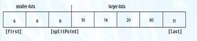
Our recursive calls to Quicksort use this index (splitPoint) to reduce the size of the problem in the general case.

Quicksort(first, splitPoint-1) sorts the left “half” of the data; Quicksort(splitPoint+1,last) sorts the right “half” of the data. (Note that the “halves” are not necessarily the same size.) splitVal is already in its correct position in data[splitPoint].

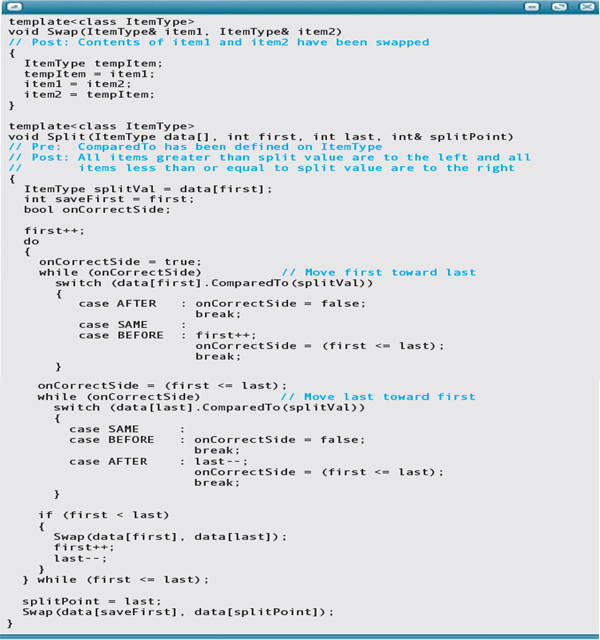
What is the base case? When the segment being examined has only one item, we do not need to go on. So “there is more than one item in data[first]..data[last]” translates into “if (first < last)”. We can now code the function Quicksort.

template<class ItemType>
void Quicksort(ItemType data[], int first, int last)
// Pre: ComparedTo has been defined on ItemType
// Post: data are sorted
{
  if (first < last)
  {
    int splitPoint;
    Split(data, first, last, splitPoint);
    // data[first]..data[splitPoint-1] <= splitVal
    // data[splitPoint] = splitVal
    // data[splitPoint+1]..data[last] > splitVal
    QuickSort(data, first, splitPoint-1);
    QuickSort(data, splitPoint+1, last);
  }
}

Now we must find a way to get all of the elements that are equal to or less than splitVal on one side of splitVal and all of the elements that are greater than splitVal on the other side. We do so by moving a pair of the indexes toward the middle of the data, looking for items that are on the wrong side of the split point. When we find pairs that are on the wrong side, we swap them and continue working our way into the middle of the data.

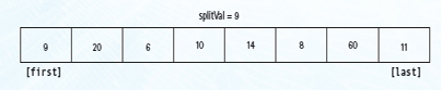
FIGURE 18.7A shows the initial state of the array to be sorted. We start out by moving first to the right, toward the middle, comparing data[first] to splitVal. If data[first] is less or equal to splitVal, we keep incrementing first; otherwise, we leave first where it is and begin moving last toward the middle. (See FIGURE 18.7B.)

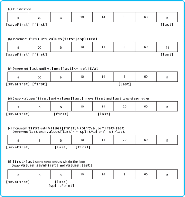
Figure 18.7 Function Split

Now data[last] is compared to splitVal. If it is greater, we continue decrementing last; otherwise, we leave last in place (see FIGURE 18.7c). At this point it is clear that data[last] and data[first] are on the wrong sides of the array. Note that the elements to the left of data[first] and to the right of data[last] are not necessarily sorted; they are just on the correct side with respect to splitVal. To move data[first] and data[last] to the correct sides, we merely swap them, and then increment first and decrement last (see FIGURE 18.7d).

Now we repeat the whole cycle, incrementing first until we encounter a value that is greater than splitVal, and then decrementing last until we encounter a value that is less than or equal to splitVal (see FIGURE 18.7e).

When does the process stop? When first and last meet each other, no additional swaps are necessary. They meet at the splitPoint. This is the location where splitVal belongs, so we swap data[saveFirst], which contains splitVal, with the element at data[splitPoint] (FIGURE 18.7f). The index splitPoint is returned from the function, to be used by Quicksort to set up the next recursive call.

To make the Quicksort function template truly generic, let's assume that the items to be sorted can be compared with the ComparedTo function.

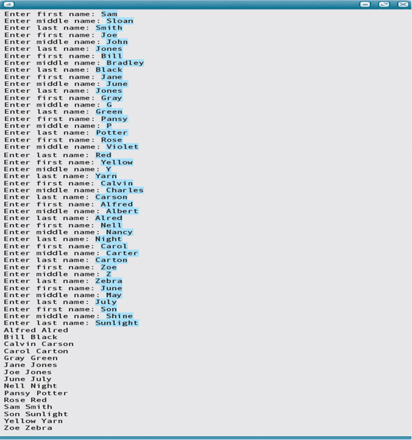
TESTING: These three functions are placed in a single file and included in a driver to be tested. Class Name defines ComparedTo, so let's read in names, sort them, and print them. Here is the driver and output from the run:

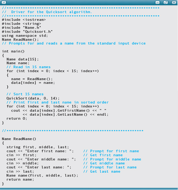
Sample run:

Testing and Debugging

Recursion is a powerful technique when it is used correctly. When improperly used, however, recursion can lead to difficult-to-diagnose errors. The best way to debug a recursive algorithm is to construct it correctly in the first place. To be realistic, we give a few hints about where to look if an error occurs.

Testing and Debugging Hints

1. Be sure there is a base case. If there is no base case, the algorithm continues to issue recursive calls until all memory has been used. Each time the function is called, either recursively or nonrecursively, stack space is allocated for the parameters and automatic local variables. If there is no base case to end the recursive calls, the run-time stack eventually overflows. An error message such as “Stack overflow” indicates that the base case is missing.

2. Make sure you have not used a While structure. The basic structure in a recursive algorithm is the If statement. There must be at least two cases: the recursive case and the base case. If the base case does nothing, the else-clause is omitted. The selection structure, however, must be present. If a While statement is used in a recursive algorithm, the While statement usually should not contain a recursive call.

3. As with nonrecursive functions, do not reference global variables directly within a recursive function unless you have justification for doing so.

4. Parameters that relate to the size of the problem must be value parameters, not reference parameters. The arguments that relate to the size of the problem are usually expressions. Arbitrary expressions can be passed only to value parameters.

5. Use your system's debugger program (or use debug output statements) to trace a series of recursive calls. Inspecting the values of parameters and local variables often helps to pinpoint the locations of errors in a recursive algorithm.

Summary

A recursive algorithm is expressed in terms of a smaller instance of itself. It must include a recursive case, for which the algorithm is expressed in terms of itself, and a base case, for which the algorithm is expressed in nonrecursive terms.

In many recursive problems, the smaller instance refers to a numeric argument that is being reduced with each call. In other problems, the smaller instance refers to the size of the data structure being manipulated. The base case is the one in which the size of the problem (in terms of either a value or a structure) reaches a point for which an explicit answer is known.

In the example of printing an array using recursion, the size of the problem was the size of the array. When the array size became 0, the entire array had been printed.

In the Towers of Hanoi game, the size of the problem was the number of discs to be moved. When only one was left on the beginning peg, it could be moved to its final destination.

Recursion incurs extra overhead that iteration doesn't. Thus, in most cases, iteration is more efficient. For some problems, however, a recursive algorithm is the natural solution. In those situations, the corresponding iterative solution is likely to be more complex— programming the iterative version often involves manually implementing the equivalent of the call stack. While you may not use recursion on a regular basis, it is a powerful tool to have in your programming toolkit.

Quick Check

1. Which case causes a recursive algorithm to end its recursion: the base case or the general case? (p. 945)

2. In writing a recursive algorithm that computes the factorial of N, what would you use as the base case? What would be the general case? (p. 947)

3. In writing a recursive algorithm that outputs the values in an array, what would you use as the base case? What would be the general case? (pp. 953–954)

4. In writing a recursive algorithm that outputs the values in linked list in reverse order, what would you use as the base case? What would be the general case? (pp. 961–962)

Answers

1. The base case. 2. The base case would be that when N is 0, the result is 1. The general case would be that when N is greater than 0, we multiply it by the product of the numbers from 1 to N - 1, as returned from a recursive call. 3. The base case would be that if there are no elements remaining, we return. The general case would be that if there are elements remaining, we print the first one, then recurse to print the rest. 4. The base case would be that the link of the current node is NULL, so we print it. The general case would be that if the link of the current node is not NULL, we print the remainder of the list before printing the current node.

Exam Preparation Exercises

1. Recursion is an alternative to

a. branching.

b. looping.

c. function invocation.

d. event handling.

2. A recursive function can be void or value returning. True or false?

3. When a function calls itself recursively, its parameters and local variables are saved on the run-time stack until it returns. True or false?

4. Tail recursion occurs when all of the processing happens at the end of the function, after the return from the recursive call. True or false?

5. Given the recursive formula F(N) = F(N - 2), with the base case F(0) = 0, what are the values of F(4), F(5), and F(6)? If any of the values are undefined, say so.

6. Given the recursive formula F(N) = F(N - 1) * 2, with the base case F(0) = 1, what are the values of F(3), F(4), and F(5)? If any of the values are undefined, say so.

7. What happens when a recursive function never encounters a base case?

8. Which practical limitation prevents a function from calling itself recursively forever?

9. A tail-recursive function would be more efficiently implemented with a loop in most cases. True or false?

10. When you develop a recursive algorithm to operate on a simple variable, what does the general case typically make smaller with each recursive call?

a. The data type of the variable

b. The number of times the variable is referenced

c. The value in the variable

11. When you develop a recursive algorithm to operate on a data structure, what does the general case typically make smaller with each recursive call?

a. The number of elements in the structure

b. The number of times the variable is referenced

c. The distance to the end of the structure

12. Given the following input data:

10
20
30

What is output by the following program?

#include <iostream>
using namespace std;
void Rev();
int main()
{
  Rev();
  return 0;
}
//*******************
void Rev()
{
  int number;
  cin >> number;
  if (cin)
  {
    Rev();
    cout << number << endl;
  }
}

13. Repeat Exercise 12, replacing the Rev function with the following version:

void Rev()
{
  int number;
  cin >> number;
  if (cin)
  {
    cout << number << endl;
    Rev();
    cout << number << endl;
  }
}

14. What is output by the following program?

#include <iostream>
using namespace std;

void Rec(string word);
int main()
{
  Rec(“abcde”);
  return 0;
}
//*******************
void Rec(string word)
{
  if (word.length() > 0)
  {
    cout << word.substr(0, 1);
    Rec(word.substr(1, word.length()-2));
    cout << word.substr(word.length()-1, 1) << endl;
  }
}

15. What does the program in Exercise 14 output if the initial call to Rec from main uses “abcdef” as the argument?

Programming Warm-Up Exercises

1. Write a value-returning recursive function called DigitSum that computes the sum of the digits in a given positive int argument. For example, if the argument is 12345, then the function returns 1 + 2 + 3 + 4 + 5 = 15.

2. Write a value-returning recursive function that uses the DigitSum function of Exercise 1 to compute the single digit to which the int argument's digits ultimately sum. For example, given the argument 999, the DigitSum result would be 9 + 9 + 9 = 27, but the recursive digit sum would then be 2 + 7 = 9.

3. Write a recursive version of a binary search of a sorted array of int values that are in ascending order. The function's arguments should be the array, the search value, and the maximum and minimum indexes for the array. The function should return the index where the match is found, or else −1.

4. Write a recursive function that asks the user to enter a positive integer number each time it is called, until zero or a negative number is input. The function then outputs the numbers entered in reverse order. For example, the I/O dialog might be the following:

Enter positive number, 0 to end: 10
Enter positive number, 0 to end: 20
Enter positive number, 0 to end: 30
Enter positive number, 0 to end: 0

The function then outputs

30
20
10

5. Extend the function of Exercise 4 so that it also outputs a running total of the numbers as they are entered. For example, the I/O dialog might be the following:

Enter positive number, 0 to end: 10
Total: 10
Enter positive number, 0 to end: 20
Total: 30
Enter positive number, 0 to end: 30
Total: 60
Enter positive number, 0 to end: 0

The function then outputs

30
20
10

6. Extend the function of Exercise 5 so that it also outputs a running total as the numbers are printed out in reverse order. For example, the I/O dialog might be the following:

Enter positive number, 0 to end: 10
Total: 10
Enter positive number, 0 to end: 20
Total: 30
Enter positive number, 0 to end: 30
Total: 60
Enter positive number, 0 to end: 0

The function then outputs

30 Total: 30
20 Total: 50
10 Total: 60

7. Extend the function of Exercise 4 so that it reports the greatest value entered, at the end of its output. For example, the I/O dialog might be the following:

Enter positive number, 0 to end: 10
Enter positive number, 0 to end: 20
Enter positive number, 0 to end: 30
Enter positive number, 0 to end: 0

The function then outputs

30
20
10
The greatest is 30

8. Change the function of Exercise 7 so that it outputs the greatest number entered thus far, as the user is entering the data. For example, the I/O dialog might be the following:

Enter positive number, 0 to end: 10
Greatest: 10
Enter positive number, 0 to end: 30
Greatest: 30

Enter positive number, 0 to end: 20
Greatest: 30
Enter positive number, 0 to end: 0

The function then outputs

20
30
10
The greatest is 30

9. Change the function of Exercise 8 so that it also outputs the greatest number thus far, as it outputs the numbers in reverse order. For example, the I/O dialog might be the following:

Enter positive number, 0 to end: 10
Greatest: 10
Enter positive number, 0 to end: 30
Greatest: 30
Enter positive number, 0 to end: 20
Greatest: 30
Enter positive number, 0 to end: 0

The function then outputs

20 Greatest: 20
30 Greatest: 30
10 Greatest: 30
The greatest is 30

10. Given the following declarations:

struct NodeType;
typedef NodeType* PtrType;
struct NodeType
{
  int info;
  PtrType link;
};
PtrType list1;
PtrType head2;

Assume that the list pointed to by list1 contains an arbitrary number of nodes. Write a recursive function that makes a copy of this list in reverse order, which is pointed to by list2.

11. Given the declarations in Exercise 10, assume that the list pointed to by list1 contains an arbitrary number of nodes. Write a recursive function that makes a copy of this list in the same order, which is pointed to by list2.

12. Given the declarations in Exercise 10, assume that the list pointed to by list1 contains an arbitrary number of nodes. Write a recursive function that makes a single list containing two copies of the list1 list. The first copy will be in the same order, and the second copy will be in reverse order. The new list is pointed to by list2.

Programming Problems

1. The greatest common divisor (GCD) of two positive integers is the largest integer that divides the numbers exactly. For example, the GCD of 14 and 21 is 7; for 13 and 22, it is 1; and for 45 and 27, it is 9. We can write a recursive formula for finding the GCD, given that the two numbers are called a and b, as:

GCD(a, b) = a, if b = 0

GCD(a, b) = GCD(b, a%b), if b > 0

Implement this recursive formula as a recursive C++ function, and write a driver program that allows you to test it interactively.

2. Write a C++ program to output the binary (base-2) representation of a decimal integer. The algorithm for this conversion is to repeatedly divide the decimal number by 2, until it is 0. Each division produces a remainder of 0 or 1, which becomes a digit in the binary number. For example, if we want the binary representation of decimal 13, we would find it with the following series of divisions:

13/2 = 6   remainder 1
6/2 = 3    remainder 0
3/2 = 1    remainder 1
1/2 = 0    remainder 1

Thus the binary representation of 13 (decimal) is 1101. The only problem with this algorithm is that the first division generates the low-order binary digit, the next division generates the second-order digit, and so on, until the last division produces the high-order digit. Thus, if we output the digits as they are generated, they will be in reverse order. You should use recursion to reverse the order of output.

3. Change the program for Problem 2 so that it works for any base up to 10. The user should enter the decimal number and the base, and the program should output the number in the given base.

4. Write a C++ program using recursion to convert a number in binary (from 1 to 10) to a decimal number. The algorithm states that each successive digit in the number is multiplied by the base (2) raised to the power corresponding to its position in the number. The low-order digit is in position 0. We sum together all of these products to get the decimal value. For example, if we have the binary number 111001, we convert it to decimal as follows:

1 * 20 = 1
0 * 21 = 0
0 * 22 = 0
1 * 23 = 8
1 * 24 = 16
1 * 25 = 32
Decimal value = 1 + 0 + 0 + 8 + 16 + 32 = 57

A recursive formulation of this algorithm can extract each digit and compute the corresponding power of the base by which to multiply. Once the base case (the last digit is extracted), the function can sum the products as it returns.

   In C++ we can represent a binary number using integers. However, there is a danger— the user can enter an invalid number by typing a digit that's unrepresentable in the base. For example, the number 1011201 is an invalid binary number because 2 isn't allowed in the binary number system. Your program should check for invalid digits as they are extracted, handle the error in an appropriate way (that is, it shouldn't output a numerical result), and provide an informative error message to the user.

5. Modify the program from Problem 4 to work for any number base in the range of 1 through 10. The user should enter a number and a base, and the program should output the decimal equivalent. If the user enters a digit that is invalid for the base, the program should output an error message and not display a numerical result.

6. A maze is to be represented by a 12 × 12 array composed of three values: Open (O), Wall (W), or Exit (E). There is one exit from the maze. Write a program to determine whether it is possible to exit the maze from each possible starting point (any open square can be a starting point). You may move vertically or horizontally to any adjacent open square. You may not move to a square containing a wall. The input consists of a series of 12 lines of 12 characters each, representing the contents of each square in the maze; the characters are O, W, or E. Your program should check that the maze has only one exit. As the data are entered, the program should make a list of all of the starting-point coordinates. It can then run through this list, solving the maze for each starting point.

Case Study Follow-Up

1. In the Problem-Solving Case Study, both sorting versions have an implicit restriction on the data type of the elements in the array. What is the restriction?

2. If the array to be sorted and/or searched combined the array and the number of elements into a struct, could the number of parameters to Sort, Search, and BinarySearch be reduced? Explain.

3. In Chapter 16, we discussed operator functions. Rewrite the Name class, replacing ComparedTo with operator functions for the relational operators.

4. Rewrite Quicksort using the relational operators. Rerun the test driver with the new Name class and Quicksort.