Now that we have understood data analysis, its process, and its installation on different platforms, it's time to learn about NumPy arrays and pandas DataFrames. This chapter acquaints you with the fundamentals of NumPy arrays and pandas DataFrames. By the end of this chapter, you will have a basic understanding of NumPy arrays, and pandas DataFrames and their related functions.

pandas is named after panel data (an econometric term) and Python data analysis and is a popular open-source Python library. We shall learn about basic pandas functionalities, data structures, and operations in this chapter. The official pandas documentation insists on naming the project pandas in all lowercase letters. The other convention the pandas project insists on is the import pandas as pd import statement.

In this chapter, our focus will be on the following topics:

• Understanding NumPy arrays
• NumPy array numerical data types
• Manipulating array shapes
• The stacking of NumPy arrays
• Partitioning NumPy arrays
• Changing the data type of NumPy arrays
• Creating NumPy views and copies
• Slicing NumPy arrays
• Boolean and fancy indexing
• Broadcasting arrays
• Creating pandas DataFrames
• Understanding pandas Series
• Reading and querying the Quandl data
• Describing pandas DataFrames

• Grouping and joining pandas DataFrames
• Working with missing values
• Creating pivot tables
• Dealing with dates

Technical requirements

This chapter has the following technical requirements:

• You can find the code and the dataset at the following GitHub link: https://github.com/PacktPublishing/Python-Data-Analysis-Third-Edition/tree/master/Chapter02.
• All the code blocks are available at ch2.ipynb.
• This chapter uses four CSV files (WHO_first9cols.csv, dest.csv, purchase.csv, and tips.csv) for practice purposes.
• In this chapter, we will use the NumPy, pandas, and Quandl Python libraries.

Understanding NumPy arrays

NumPy can be installed on a PC using pip or brew but if the user is using the Jupyter Notebook, then there is no need to install it. NumPy is already installed in the Jupyter Notebook. I will suggest to you to please use the Jupyter Notebook as your IDE because we are executing all the code in the Jupyter Notebook. We have already shown in Chapter 1, Getting Started with Python Libraries, how to install Anaconda, which is a complete suite for data analysis. NumPy arrays are a series of homogenous items. Homogenous means the array will have all the elements of the same data type. Let's create an array using NumPy. You can create an array using the array() function with a list of items. Users can also fix the data type of an array. Possible data types are bool, int, float, long, double, and long double.

Let's see how to create an empty array:

# Creating an array
import numpy as np
a = np.array([2,4,6,8,10])
print(a)

Output:
[ 2 4 6 8 10]

Another way to create a NumPy array is with arange(). It creates an evenly spaced NumPy array. Three values – start, stop, and step – can be passed to the arange(start,[stop],step) function. The start is the initial value of the range, the stop is the last value of the range, and the step is the increment in that range. The stop parameter is compulsory. In the following example, we have used 1 as the start and 11 as the stop parameter. The arange(1,11) function will return 1 to 10 values with one step because the step is, by default, 1. The arrange() function generates a value that is one less than the stop parameter value. Let's understand this through the following example:

# Creating an array using arange()
import numpy as np
a = np.arange(1,11)
print(a)

Output:
[ 1 2 3 4 5 6 7 8 9 10]

Apart from the array() and arange() functions, there are other options, such as zeros(), ones(), full(), eye(), and random(), which can also be used to create a NumPy array, as these functions are initial placeholders. Here is a detailed description of each function:

• zeros(): The zeros()function creates an array for a given dimension with all zeroes.
• ones(): The ones() function creates an array for a given dimension with all ones.
• fulls(): The full() function generates an array with constant values.
• eyes(): The eye() function creates an identity matrix.
• random(): The random() function creates an array with any given dimension.

Let's understand these functions through the following example:

import numpy as np

# Create an array of all zeros
p = np.zeros((3,3)) 
print(p) 

# Create an array of all ones
q = np.ones((2,2)) 
print(q)

# Create a constant array
r = np.full((2,2), 4) 
print(r) 

# Create a 2x2 identity matrix
s = np.eye(4) 
print(s) 

# Create an array filled with random values
t = np.random.random((3,3))
print(t)

This results in the following output:

[[0. 0. 0.]
 [0. 0. 0.]
 [0. 0. 0.]]

[[1. 1.]
 [1. 1.]]

[[4 4]
 [4 4]]

[[1. 0. 0. 0.]
 [0. 1. 0. 0.]
 [0. 0. 1. 0.]
 [0. 0. 0. 1.]]

[[0.16681892 0.00398631 0.61954178]
 [0.52461924 0.30234715 0.58848138]
 [0.75172385 0.17752708 0.12665832]]

In the preceding code, we have seen some built-in functions for creating arrays with all-zero values, all-one values, and all-constant values. After that, we have created the identity matrix using the eye() function and a random matrix using the random.random() function. Let's see some other array features in the next section.

Array features

In general, NumPy arrays are a homogeneous kind of data structure that has the same types of items. The main benefit of an array is its certainty of storage size because of its same type of items. A Python list uses a loop to iterate the elements and perform operations on them. Another benefit of NumPy arrays is to offer vectorized operations instead of iterating each item and performing operations on it. NumPy arrays are indexed just like a Python list and start from 0. NumPy uses an optimized C API for the fast processing of the array operations.

Let's make an array using the arange() function, as we did in the previous section, and let's check its data type:

# Creating an array using arange()
import numpy as np
a = np.arange(1,11)

print(type(a))
print(a.dtype)

Output:
<class 'numpy.ndarray'>
int64

When you use type(), it returns numpy.ndarray. This means that the type() function returns the type of the container. When you use dtype(), it will return int64, since it is the type of the elements. You may also get the output as int32 if you are using 32-bit Python. Both cases use integers (32- and 64-bit). One-dimensional NumPy arrays are also known as vectors.

Let's find out the shape of the vector that we produced a few minutes ago:

print(a.shape)
Output: (10,)

As you can see, the vector has 10 elements with values ranging from 1 to 10. The shape property of the array is a tuple; in this instance, it is a tuple of one element, which holds the length in each dimension.

Selecting array elements

In this section, we will see how to select the elements of the array. Let's see an example of a 2*2 matrix:

a = np.array([[5,6],[7,8]])
print(a)

Output:
[[5 6]
 [7 8]]

In the preceding example, the matrix is created using the array() function with the input list of lists.

Selecting array elements is pretty simple. We just need to specify the index of the matrix as a[m,n]. Here, m is the row index and n is the column index of the matrix. We will now select each item of the matrix one by one as shown in the following code:

print(a[0,0])
Output: 5

print(a[0,1])
Output: 6

printa([1,0])
Output: 7

printa([1,1])
Output: 8

In the preceding code sample, we have tried to access each element of an array using array indices. You can also understand this by the diagram mentioned here:

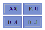
In the preceding diagram, we can see it has four blocks and each block represents the element of an array. The values written in each block show its indices.

In this section, we have understood the fundamentals of arrays. Now, let's jump to arrays of numerical data types.

NumPy array numerical data types

Python offers three types of numerical data types: integer type, float type, and complex type. In practice, we need more data types for scientific computing operations with precision, range, and size. NumPy offers a bulk of data types with mathematical types and numbers. Let's see the following table of NumPy numerical types:

For each data type, there exists a matching conversion function:

print(np.float64(21))
Output: 21.0

print(np.int8(21.0))
Output: 42

print(np.bool(21))
Output: True

print(np.bool(0))
Output: False

print(np.bool(21.0))
Output: True

print(np.float(True))
Output: 1.0

print(np.float(False))
Output: 0.0

Many functions have a data type argument, which is frequently optional:

arr=np.arange(1,11, dtype= np.float32)
print(arr)

Output:  
[ 1. 2. 3. 4. 5. 6. 7. 8. 9. 10.]

It is important to be aware that you are not allowed to change a complex number into an integer. If you try to convert complex data types into integers, then you will get TypeError. Let's see the following example:

np.int(42.0 + 1.j)

This results in the following output:

You will get the same error if you try the conversion of a complex number into a floating point.

But you can convert float values into complex numbers by setting individual pieces. You can also pull out the pieces using the real and imag attributes. Let's see that using the following example:

c= complex(42, 1)
print(c)

Output: (42+1j)

print(c.real,c.imag)

Output: 42.0 1.0

In the preceding example, you have defined a complex number using the complex() method. Also, you have extracted the real and imaginary values using the real and imag attributes. Let's now jump to dtype objects.

dtype objects

We have seen in earlier sections of the chapter that dtype tells us the type of individual elements of an array. NumPy array elements have the same data type, which means that all elements have the same dtype. dtype objects are instances of the numpy.dtype class:

# Creating an array
import numpy as np
a = np.array([2,4,6,8,10])

print(a.dtype)
Output: 'int64'

dtype objects also tell us the size of the data type in bytes using the itemsize property:

print(a.dtype.itemsize)
Output:8

Data type character codes

# Create numpy array using arange() function
var1=np.arange(1,11, dtype='f')
print(var1)

Output:
[ 1.,  2.,  3.,  4.,  5.,  6.,  7.,  8.,  9., 10.]

print(np.arange(1,6, dtype='D'))

Output:
[1.+0.j, 2.+0.j, 3.+0.j, 4.+0.j, 5.+0.j]

dtype constructors

There are lots of ways to create data types using constructors. Constructors are used to instantiate or assign a value to an object. In this section, we will understand data type creation with the help of a floating-point data example:

• To try out a general Python float, use the following:

print(np.dtype(float))
Output: float64

• To try out a single-precision float with a character code, use the following:

print(np.dtype('f'))
Output: float32

• To try out a double-precision float with a character code, use the following:

print(np.dtype('d'))
Output: float64

• To try out a dtype constructor with a two-character code, use the following:

print(np.dtype('f8'))
Output: float64

Here, the first character stands for the type and a second character is a number specifying the number of bytes in the type, for example, 2, 4, or 8.

dtype attributes

The dtype class offers several useful attributes. For example, we can get information about the character code of a data type using the dtype attribute:

# Create numpy array 
var2=np.array([1,2,3],dtype='float64')

print(var2.dtype.char)

Output: 'd'

The type attribute corresponds to the type of object of the array elements:

print(var2.dtype.type)

Output: <class 'numpy.float64'>

Now that we know all about the various data types used in NumPy arrays, let's start manipulating them in the next section.

Manipulating array shapes

In this section, our main focus is on array manipulation. Let's learn some new Python functions of NumPy, such as reshape(), flatten(), ravel(), transpose(), and resize():

• reshape() will change the shape of the array:

# Create an array
arr = np.arange(12)
print(arr)

Output: [ 0  1  2  3  4  5  6  7  8  9 10 11]

# Reshape the array dimension
new_arr=arr.reshape(4,3)

print(new_arr)

Output: [[ 0,  1,  2],
               [ 3,  4,  5],
               [ 6,  7,  8],
               [ 9, 10, 11]]

# Reshape the array dimension
new_arr2=arr.reshape(3,4)

print(new_arr2)

Output:
array([[ 0,  1,  2,  3],
       [ 4,  5,  6,  7],
       [ 8,  9, 10, 11]])

• Another operation that can be applied to arrays is flatten(). flatten() transforms an n-dimensional array into a one-dimensional array:

# Create an array
arr=np.arange(1,10).reshape(3,3)
print(arr)

Output: 
[[1 2 3]
 [4 5 6]
 [7 8 9]]

print(arr.flatten())

Output: 
[1 2 3 4 5 6 7 8 9]

• The ravel() function is similar to the flatten() function. It also transforms an n-dimensional array into a one-dimensional array. The main difference is that flatten() returns the actual array while ravel() returns the reference of the original array. The ravel() function is faster than the flatten() function because it does not occupy extra memory:

print(arr.ravel())

Output: 
[1, 2, 3, 4, 5, 6, 7, 8, 9]

• The transpose() function is a linear algebraic function that transposes the given two-dimensional matrix. The word transpose means converting rows into columns and columns into rows:

# Transpose the matrix
print(arr.transpose())

Output:
[[1 4 7]
 [2 5 8]
 [3 6 9]]

• The resize() function changes the size of the NumPy array. It is similar to reshape() but it changes the shape of the original array:

# resize the matrix
arr.resize(1,9)
print(arr)

Output:[[1 2 3 4 5 6 7 8 9]]

In all the code in this section, we have seen built-in functions such as reshape(), flatten(), ravel(), transpose(), and resize() for manipulating size. Now, it's time to learn about the stacking of NumPy arrays.

The stacking of NumPy arrays

NumPy offers a stack of arrays. Stacking means joining the same dimensional arrays along with a new axis. Stacking can be done horizontally, vertically, column-wise, row-wise, or depth-wise:

• Horizontal stacking: In horizontal stacking, the same dimensional arrays are joined along with a horizontal axis using the hstack() and concatenate() functions. Let's see the following example:

arr1 = np.arange(1,10).reshape(3,3)
print(arr1)

Output:
[[1 2 3]
 [4 5 6]
 [7 8 9]]

We have created one 3*3 array; it's time to create another 3*3 array:

arr2 = 2*arr1
print(arr2)

Output:
[[ 2 4 6]
 [ 8 10 12]
 [14 16 18]]

After creating two arrays, we will perform horizontal stacking:

# Horizontal Stacking
arr3=np.hstack((arr1, arr2))
print(arr3)

Output:
[[ 1 2 3 2 4 6]
 [ 4 5 6 8 10 12]
 [ 7 8 9 14 16 18]]

In the preceding code, two arrays are stacked horizontally along the x axis. The concatenate() function can also be used to generate the horizontal stacking with axis parameter value 1:

# Horizontal stacking using concatenate() function
arr4=np.concatenate((arr1, arr2), axis=1)
print(arr4)

Output:
[[ 1 2 3 2 4 6]
 [ 4 5 6 8 10 12]
 [ 7 8 9 14 16 18]]

In the preceding code, two arrays have been stacked horizontally using the concatenate() function.

• Vertical stacking: In vertical stacking, the same dimensional arrays are joined along with a vertical axis using the vstack() and concatenate() functions. Let's see the following example:

# Vertical stacking
arr5=np.vstack((arr1, arr2))
print(arr5)

Output:
[[ 1 2 3]
 [ 4 5 6]
 [ 7 8 9]
 [ 2 4 6]
 [ 8 10 12]
 [14 16 18]]

In the preceding code, two arrays are stacked vertically along the y axis. The concatenate() function can also be used to generate vertical stacking with axis parameter value 0:

arr6=np.concatenate((arr1, arr2), axis=0) 
print(arr6)

Output:
[[ 1 2 3]
 [ 4 5 6]
 [ 7 8 9]
 [ 2 4 6]
 [ 8 10 12]
 [14 16 18]]

In the preceding code, two arrays are stacked vertically using the concatenate() function.

• Depth stacking: In depth stacking, the same dimensional arrays are joined along with a third axis (depth) using the dstack() function. Let's see the following example:

arr7=np.dstack((arr1, arr2))
print(arr7)

Output:
[[[ 1 2]
  [ 2 4]
  [ 3 6]]

 [[ 4 8]
  [ 5 10]
  [ 6 12]]

 [[ 7 14]
  [ 8 16]
  [ 9 18]]]

In the preceding code, two arrays are stacked in depth along with a third axis (depth).

• Column stacking: Column stacking stacks multiple sequence one-dimensional arrays as columns into a single two-dimensional array. Let's see an example of column stacking:

# Create 1-D array
arr1 = np.arange(4,7) 
print(arr1)

Output: [4, 5, 6]

In the preceding code block, we have created a one-dimensional NumPy array.

# Create 1-D array
arr2 = 2 * arr1
print(arr2)

Output: [ 8, 10, 12]

In the preceding code block, we have created another one-dimensional NumPy array.

# Create column stack
arr_col_stack=np.column_stack((arr1,arr2))
print(arr_col_stack)

Output:
[[ 4 8]
 [ 5 10]
 [ 6 12]]

In the preceding code, we have created two one-dimensional arrays and stacked them column-wise.

• Row stacking: Row stacking stacks multiple sequence one-dimensional arrays as rows into a single two-dimensional arrays. Let's see an example of row stacking:

# Create row stack
arr_row_stack = np.row_stack((arr1,arr2)) 
print(arr_row_stack)

Output:
[[ 4 5 6]
 [ 8 10 12]]

In the preceding code, two one-dimensional arrays are stacked row-wise.

Let's now see how to partition a NumPy array into multiple sub-arrays.

Partitioning NumPy arrays

NumPy arrays can be partitioned into multiple sub-arrays. NumPy offers three types of split functionality: vertical, horizontal, and depth-wise. All the split functions by default split into the same size arrays but we can also specify the split location. Let's look at each of the functions in detail:

• Horizontal splitting: In horizontal split, the given array is divided into N equal sub-arrays along the horizontal axis using the hsplit() function. Let's see how to split an array:

# Create an array
arr=np.arange(1,10).reshape(3,3)
print(arr)

Output: 
[[1 2 3]
 [4 5 6]
 [7 8 9]]

# Peroform horizontal splitting
arr_hor_split=np.hsplit(arr, 3)

print(arr_hor_split)

Output:
[array([[1],
       [4],
       [7]]), array([[2],
       [5],
       [8]]), array([[3],
       [6],
       [9]])]

In the preceding code, the hsplit(arr, 3) function divides the array into three sub-arrays. Each part is a column of the original array.

• Vertical splitting: In vertical split, the given array is divided into N equal sub-arrays along the vertical axis using the vsplit() and split() functions. The split function with axis=0 performs the same operation as the vsplit() function:

# vertical split
arr_ver_split=np.vsplit(arr, 3)

print(arr_ver_split)

Output:
[array([[1, 2, 3]]), array([[4, 5, 6]]), array([[7, 8, 9]])]

In the preceding code, the vsplit(arr, 3) function divides the array into three sub-arrays. Each part is a row of the original array. Let's see another function, split(), which can be utilized as a vertical and horizontal split, in the following example:

# split with axis=0
arr_split=np.split(arr,3,axis=0)

print(arr_split)

Output:
[array([[1, 2, 3]]), array([[4, 5, 6]]), array([[7, 8, 9]])]

# split with axis=1
arr_split = np.split(arr,3,axis=1)

Output:
[array([[1],
        [4],
        [7]]), array([[2],
        [5],
        [8]]), array([[3],
        [6],
        [9]])]

In the preceding code, the split(arr, 3) function divides the array into three sub-arrays. Each part is a row of the original array. The split output is similar to the vsplit() function when axis=0 and the split output is similar to the hsplit() function when axis=1.

Changing the data type of NumPy arrays

As we have seen in the preceding sections, NumPy supports multiple data types, such as int, float, and complex numbers. The astype() function converts the data type of the array. Let's see an example of the astype() function:

# Create an array
arr=np.arange(1,10).reshape(3,3)
print("Integer Array:",arr)

# Change datatype of array
arr=arr.astype(float)

# print array
print("Float Array:", arr)

# Check new data type of array
print("Changed Datatype:", arr.dtype)

In the preceding code, we have created one NumPy array and checked its data type using the dtype attribute.

Let's change the data type of an array using the astype() function:

# Change datatype of array
arr=arr.astype(float)

# Check new data type of array
print(arr.dtype)

Output:
float64

In the preceding code, we have changed the column data type from integer to float using astype().

The tolist() function converts a NumPy array into a Python list. Let's see an example of the tolist() function:

# Create an array
arr=np.arange(1,10)

# Convert NumPy array to Python List
list1=arr.tolist()
print(list1)

Output:
[1, 2, 3, 4, 5, 6, 7, 8, 9]

In the preceding code, we have converted an array into a Python list object using the tolist() function.

Creating NumPy views and copies

Some of the Python functions return either a copy or a view of the input array. A Python copy stores the array in another location while a view uses the same memory content. This means copies are separate objects and treated as a deep copy in Python. Views are the original base array and are treated as a shallow copy. Here are some properties of copies and views:

• Modifications in a view affect the original data whereas modifications in a copy do not affect the original array.
• Views use the concept of shared memory.
• Copies require extra space compared to views.
• Copies are slower than views.

Let's understand the concept of copy and view using the following example:

# Create NumPy Array
arr = np.arange(1,5).reshape(2,2)
print(arr)

Output:
[[1, 2],
[3, 4]]

After creating a NumPy array, let's perform object copy operations:

# Create no copy only assignment
arr_no_copy=arr

# Create Deep Copy
arr_copy=arr.copy()

# Create shallow copy using View
arr_view=arr.view()

print("Original Array: ",id(arr))
print("Assignment: ",id(arr_no_copy))
print("Deep Copy: ",id(arr_copy))
print("Shallow Copy(View): ",id(arr_view))

Output:
Original Array:  140426327484256
Assignment:  140426327484256
Deep Copy:  140426327483856
Shallow Copy(View):  140426327484496

In the preceding example, you can see the original array and the assigned array have the same object ID, meaning both are pointing to the same object. Copies and views both have different object IDs; both will have different objects, but view objects will reference the same original array and a copy will have a different replica of the object.

Let's continue with this example and update the values of the original array and check its impact on views and copies:

# Update the values of original array
arr[1]=[99,89]

# Check values of array view
print("View Array:
", arr_view)

# Check values of array copy
print("Copied Array:
", arr_copy)

Output: 
View Array:
 [[ 1 2]
 [99 89]]
Copied Array:
 [[1 2]
 [3 4]]

In the preceding example, we can conclude from the results that the view is the original array. The values changed when we updated the original array and the copy is a separate object because its values remain the same.

Slicing NumPy arrays

Slicing in NumPy is similar to Python lists. Indexing prefers to select a single value while slicing is used to select multiple values from an array.

NumPy arrays also support negative indexing and slicing. Here, the negative sign indicates the opposite direction and indexing starts from the right-hand side with a starting value of -1:

Let's check this out using the following code:

# Create NumPy Array
arr = np.arange(0,10)
print(arr)

Output: [0, 1, 2, 3, 4, 5, 6, 7, 8, 9]

In the slice operation, we use the colon symbol to select the collection of values. Slicing takes three values: start, stop, and step:

print(arr[3:6])
Output: [3, 4, 5]

This can be represented as follows:

In the preceding example, we have used 3 as the starting index and 6 as the stopping index:

print(arr[3:])
Output: array([3, 4, 5, 6, 7, 8, 9])

In the preceding example, only the starting index is given. 3 is the starting index. This slice operation will select the values from the starting index to the end of the array:

print(arr[-3:])
Output: array([7, 8, 9])

This can be represented as follows:

In the preceding example, the slice operation will select values from the third value from the right side of the array to the end of the array:

print(arr[2:7:2])
Output: array([2, 4,6])

This can be represented as follows:

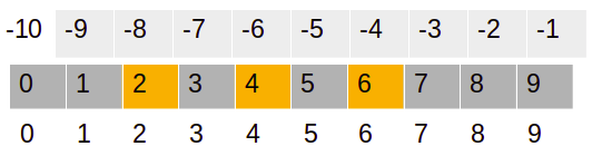
In the preceding example, the start, stop, and step index are 2, 7, and 2, respectively. Here, the slice operation selects values from the second index to the sixth (one less than the stop value) index with an increment of 2 in the index value. So, the output will be 2, 4, and 6.

Boolean and fancy indexing

Indexing techniques help us to select and filter elements from a NumPy array. In this section, we will focus on Boolean and fancy indexing. Boolean indexing uses a Boolean expression in the place of indexes (in square brackets) to filter the NumPy array. This indexing returns elements that have a true value for the Boolean expression:

# Create NumPy Array
arr = np.arange(21,41,2)
print("Orignial Array:
",arr)

# Boolean Indexing
print("After Boolean Condition:",arr[arr>30])

Output:
Orignial Array:
 [21 23 25 27 29 31 33 35 37 39]
After Boolean Condition: [31 33 35 37 39]

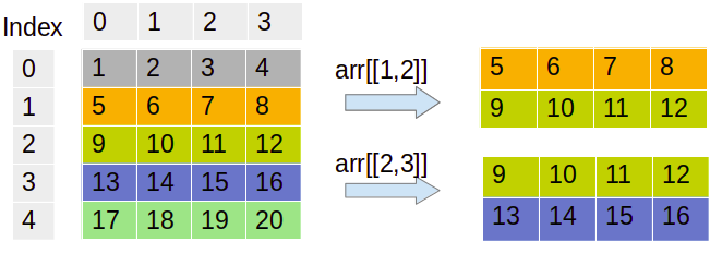
Fancy indexing is a special type of indexing in which elements of an array are selected by an array of indices. This means we pass the array of indices in brackets. Fancy indexing also supports multi-dimensional arrays. This will help us to easily select and modify a complex multi-dimensional set of arrays. Let's see an example as follows to understand fancy indexing:

# Create NumPy Array
arr = np.arange(1,21).reshape(5,4)
print("Orignial Array:
",arr)

# Selecting 2nd and 3rd row
indices = [1,2]
print("Selected 1st and 2nd Row:
", arr[indices])

# Selecting 3nd and 4th row
indices = [2,3]
print("Selected 3rd and 4th Row:
", arr[indices])

Output:

Orignial Array:
 [[ 1 2 3 4]
 [ 5 6 7 8]
 [ 9 10 11 12]
 [13 14 15 16]
 [17 18 19 20]]
Selected 1st and 2nd Row:
 [[ 5 6 7 8]
 [ 9 10 11 12]]
Selected 3rd and 4th Row:
 [[ 9 10 11 12]
 [13 14 15 16]]

In the preceding code, we have created a 5*4 matrix and selected the rows using integer indices. You can also visualize or internalize this output from the following diagram:

We can see the code for this as follows:

# Create row and column indices
row = np.array([1, 2])
col = np.array([2, 3])

print("Selected Sub-Array:", arr[row, col])

Output:
Selected Sub-Array: [ 7 12]

The preceding example results in the first value, [1,2], and second value, [2,3], as the row and column index. The array will select the value at the first and second index values, which are 7 and 12.

Broadcasting arrays

Python lists do not support direct vectorizing arithmetic operations. NumPy offers a faster-vectorized array operation compared to Python list loop-based operations. Here, all the looping operations are performed in C instead of Python, which makes it faster. Broadcasting functionality checks a set of rules for applying binary functions, such as addition, subtraction, and multiplication, on different shapes of an array.

Let's see an example of broadcasting:

# Create NumPy Array
arr1 = np.arange(1,5).reshape(2,2) 
print(arr1)

Output:
[[1 2]
 [3 4]]

# Create another NumPy Array
arr2 = np.arange(5,9).reshape(2,2) 
print(arr2)

Output:
[[5 6]
 [7 8]]

# Add two matrices
print(arr1+arr2)

Output:
[[ 6 8]
 [10 12]]

In all three preceding examples, we can see the addition of two arrays of the same size. This concept is known as broadcasting:

# Multiply two matrices
print(arr1*arr2)

Output:
[[ 5 12]
 [21 32]]

In the preceding example, two matrices were multiplied. Let's perform addition and multiplication with a scalar value:

# Add a scaler value
print(arr1 + 3)

Output:
[[4 5]
 [6 7]]

# Multiply with a scalar value
print(arr1 * 3)

Output:
[[ 3 6]
 [ 9 12]]

In the preceding two examples, the matrix is added and multiplied by a scalar value.

Creating pandas DataFrames

The pandas library is designed to work with a panel or tabular data. pandas is a fast, highly efficient, and productive tool for manipulating and analyzing string, numeric, datetime, and time-series data. pandas provides data structures such as DataFrames and Series. A pandas DataFrame is a tabular, two-dimensional labeled and indexed data structure with a grid of rows and columns. Its columns are heterogeneous types. It has the capability to work with different types of objects, carry out grouping and joining operations, handle missing values, create pivot tables, and deal with dates. A pandas DataFrame can be created in multiple ways. Let's create an empty DataFrame:

# Import pandas library
import pandas as pd

# Create empty DataFrame
df = pd.DataFrame()

# Header of dataframe. 
df.head()

Output:
_ 

In the preceding example, we have created an empty DataFrame. Let's create a DataFrame using a dictionary of the list:

# Create dictionary of list
data = {'Name': ['Vijay', 'Sundar', 'Satyam', 'Indira'], 'Age': [23, 45, 46, 52 ]}  

# Create the pandas DataFrame
df = pd.DataFrame(data)

# Header of dataframe.
df.head()

Output:
  Name Age
0 Vijay 23
1 Sundar 45
2 Satyam 46
3 Indira 52

In the preceding code, we have used a dictionary of the list to create a DataFrame. Here, the keys of the dictionary are equivalent to columns, and values are represented as a list that is equivalent to the rows of the DataFrame. Let's create a DataFrame using the list of dictionaries:

# Pandas DataFrame by lists of dicts. 
# Initialise data to lists. 
data =[ {'Name': 'Vijay', 'Age': 23},{'Name': 'Sundar', 'Age': 25},{'Name': 'Shankar', 'Age': 26}]

# Creates DataFrame. 
df = pd.DataFrame(data,columns=['Name','Age']) 

# Print dataframe header 
df.head() 

In the preceding code, the DataFrame is created using a list of dictionaries. In the list, each item is a dictionary. Each key is the name of the column and the value is the cell value for a row. Let's create a DataFrame using a list of tuples:

# Creating DataFrame using list of tuples.
data = [('Vijay', 23),( 'Sundar', 45), ('Satyam', 46), ('Indira',52)]

# Create dataframe
df = pd.DataFrame(data, columns=['Name','Age'])

# Print dataframe header
df.head() 

Output:
  Name Age
0 Vijay 23
1 Sundar 25
2 Shankar 26

In the preceding code, the DataFrame is created using a list of tuples. In the list, each item is a tuple and each tuple is equivalent to the row of columns.

Understanding pandas Series

pandas Series is a one-dimensional sequential data structure that is able to handle any type of data, such as string, numeric, datetime, Python lists, and dictionaries with labels and indexes. Series is one of the columns of a DataFrame. We can create a Series using a Python dictionary, NumPy array, and scalar value. We will also see the pandas Series features and properties in the latter part of the section. Let's create some Python Series:

• Using a Python dictionary: Create a dictionary object and pass it to the Series object. Let's see the following example:

# Creating Pandas Series using Dictionary
dict1 = {0 : 'Ajay', 1 : 'Jay', 2 : 'Vijay'}

# Create Pandas Series
series = pd.Series(dict1)

# Show series
series

Output:
0     Ajay
1      Jay
2    Vijay
dtype: object

• Using a NumPy array: Create a NumPy array object and pass it to the Series object. Let's see the following example:

#Load Pandas and NumPy libraries
import pandas as pd
import numpy as np

# Create NumPy array
arr = np.array([51,65,48,59, 68])

# Create Pandas Series
series = pd.Series(arr)
series

Output:
0    51
1    65
2    48
3    59
4    68
dtype: int64

• Using a single scalar value: To create a pandas Series with a scalar value, pass the scalar value and index list to a Series object:

# load Pandas and NumPy
import pandas as pd
import numpy as np

# Create Pandas Series
series = pd.Series(10, index=[0, 1, 2, 3, 4, 5])
series

Output:
0    10
1    10
2    10
3    10
4    10
5    10
dtype: int64

Let's explore some features of pandas Series:

• We can also create a series by selecting a column, such as country, which happens to be the first column in the datafile. Then, show the type of the object currently in the local scope:

# Import pandas
import pandas as pd

# Load data using read_csv()
df = pd.read_csv("WHO_first9cols.csv")

# Show initial 5 records
df.head()

This results in the following output:

In the preceding code, we have read the WHO_first9cols.csv file using the read_csv() function. You can download this file from the following GitHub location:https://github.com/PacktPublishing/Python-Data-Analysis-Third-Edition/tree/master/Chapter02. In the output, you can see the top five records in the WHO_first9cols dataset using the head() function:

# Select a series
country_series=df['Country']

# check datatype of series
type(country_series)

Output:
pandas.core.series.Series

• The pandas Series data structure shares some of the common attributes of DataFrames and also has a name attribute. Explore these properties as follows:

# Show the shape of DataFrame
print("Shape:", df.shape)

Output:
Shape: (202, 9)

Let's check the column list of a DataFrame:

# Check the column list of DataFrame
print("List of Columns:", df.columns)

Output:List of Columns: Index(['Country', 'CountryID', 'Continent', 'Adolescent fertility rate (%)',
       'Adult literacy rate (%)',
       'Gross national income per capita (PPP international $)',
       'Net primary school enrolment ratio female (%)',
       'Net primary school enrolment ratio male (%)',
       'Population (in thousands) total'],
       dtype='object')

Let's check the data types of DataFrame columns:

# Show the datatypes of columns
print("Data types:", df.dtypes)

Output:
Data types: Country                                                    object
            CountryID                                                   int64
            Continent                                                   int64
            Adolescent fertility rate (%)                             float64
            Adult literacy rate (%)                                   float64
            Gross national income per capita (PPP international $)    float64
            Net primary school enrolment ratio female (%)             float64
            Net primary school enrolment ratio male (%)               float64
            Population (in thousands) total                           float64
            dtype: object

3. Let's see the slicing of a pandas Series:

# Pandas Series Slicing
country_series[-5:]

Output:
197               Vietnam
198    West Bank and Gaza
199                 Yemen
200                Zambia
201              Zimbabwe
Name: Country, dtype: object

Now that we know how to use pandas Series, let's move on to using Quandl to work on databases.

Reading and querying the Quandl data

In the last section, we saw pandas DataFrames that have a tabular structure similar to relational databases. They offer similar query operations on DataFrames. In this section, we will focus on Quandl. Quandl is a Canada-based company that offers commercial and alternative financial data for investment data analyst. Quandl understands the need for investment and financial quantitative analysts. It provides data using API, R, Python, or Excel.

In this section, we will retrieve the Sunspot dataset from Quandl. We can use either an API or download the data manually in CSV format.

Let's first install the Quandl package using pip:

$ pip3 install Quandl

If you want to install the API, you can do so by downloading installers from https://pypi.python.org/pypi/Quandl or by running the preceding command.

Let's take a look at how to query data in a pandas DataFrame:

1. As a first step, we obviously have to download the data. After importing the Quandl API, get the data as follows:

import quandl
sunspots = quandl.get("SIDC/SUNSPOTS_A")

2. The head() and tail() methods have a purpose similar to that of the Unix commands with the same name. Select the first n and last n records of a DataFrame, where n is an integer parameter:

sunspots.head()

This results in the following output:

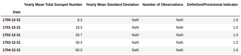
Let's check out the tail function as follows:

sunspots.tail()

This results in the following output:

The head() and tail() methods give us the first and last five rows of the Sunspot data, respectively.

3. Filtering columns: pandas offers the ability to select columns. Let's select columns in a pandas DataFrame:

# Select columns
sunspots_filtered=sunspots[['Yearly Mean Total Sunspot Number','Definitive/Provisional Indicator']]

# Show top 5 records
sunspots_filtered.head()

This results in the following output:

4. Filtering rows: pandas offers the ability to select rows. Let's select rows in a pandas DataFrame:

# Select rows using index
sunspots["20020101": "20131231"]

This results in the following output:

5. Boolean filtering: We can query data using Boolean conditions similar to the WHERE clause condition of SQL. Let's filter the data greater than the arithmetic mean:

# Boolean Filter
sunspots[sunspots['Yearly Mean Total Sunspot Number'] > sunspots['Yearly Mean Total Sunspot Number'].mean()]

This results in the following output:

Describing pandas DataFrames

The pandas DataFrame has a dozen statistical methods. The following table lists these methods, along with a short description of each:

Using the same data used in the previous section, we will demonstrate these statistical methods:

# Describe the dataset
df.describe()

This results in the following output:

The describe() method will show most of the descriptive statistical measures for all columns:

# Count number of observation
df.count()

This results in the following output:

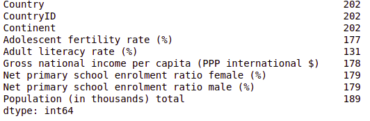
The count() method counts the number of observations in each column. It helps us to check the missing values in the dataset. Except for the initial three columns, all the columns have missing values. Similarly, you can compute the median, standard deviation, mean absolute deviation, variance, skewness, and kurtosis:

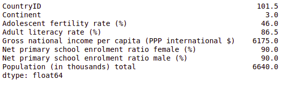
# Compute median of all the columns
df.median()

This results in the following output:

We can compute deviation for all columns as follows:

# Compute the standard deviation of all the columns
df.std()

This results in the following output:

The preceding code example is computing the standard deviation for each numeric column.

Grouping and joining pandas DataFrame

Grouping is a kind of data aggregation operation. The grouping term is taken from a relational database. Relational database software uses the group by keyword to group similar kinds of values in a column. We can apply aggregate functions on groups such as mean, min, max, count, and sum. The pandas DataFrame also offers similar kinds of capabilities. Grouping operations are based on the split-apply-combine strategy. It first divides data into groups and applies the aggregate operation, such as mean, min, max, count, and sum, on each group and combines results from each group:

# Group By DataFrame on the basis of Continent column
df.groupby('Continent').mean()

This results in the following output:

Let's now group the DataFrames based on literacy rates as well:

# Group By DataFrame on the basis of continent and select adult literacy rate(%)
df.groupby('Continent').mean()['Adult literacy rate (%)']

This results in the following output:

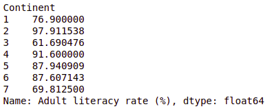
In the preceding example, the continent-wise average adult literacy rate in percentage was computed. You can also group based on multiple columns by passing a list of columns to the groupby() function.

Join is a kind of merge operation for tabular databases. The join concept is taken from the relational database. In relational databases, tables were normalized or broken down to reduce redundancy and inconsistency, and join is used to select the information from multiple tables. A data analyst needs to combine data from multiple sources. pandas also offers to join functionality to join multiple DataFrames using the merge() function.

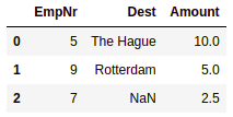
To understand joining, we will take a taxi company use case. We are using two files: dest.csv and tips.csv. Every time a driver drops any passenger at their destination, we will insert a record (employee number and destination) into the dest.csv file. Whenever drivers get a tip, we insert the record (employee number and tip amount) into the tips.csv file. You can download both the files from the following GitHub link: https://github.com/PacktPublishing/Python-Data-Analysis-Third-Edition/tree/master/Python-Data-Analysis-Third-Edition/Ch2:

# Import pandas
import pandas as pd

# Load data using read_csv()
dest = pd.read_csv("dest.csv")

# Show DataFrame
dest.head()

This results in the following output:

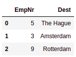
In the preceding code block, we have read the dest.csv file using the read_csv() method:

# Load data using read_csv()
tips = pd.read_csv("tips.csv")

# Show DataFrame
tips.head()

This results in the following output:

In the preceding code block, we have read the tips.csv file using the read_csv() method. We will now check out the various types of joins as follows:

• Inner join: Inner join is equivalent to the intersection operation of a set. It will select only common records in both the DataFrames. To perform inner join, use the merge() function with both the DataFrames and common attribute on the parameter and inner value to show the parameter. The on parameter is used to provide the common attribute based on the join will be performed and how defines the type of join:

# Join DataFrames using Inner Join
df_inner= pd.merge(dest, tips, on='EmpNr', how='inner')
df_inner.head()

This results in the following output:

• Full outer join: Outer join is equivalent to a union operation of the set. It merges the right and left DataFrames. It will have all the records from both DataFrames and fills NaNs where the match will not be found:

# Join DataFrames using Outer Join
df_outer= pd.merge(dest, tips, on='EmpNr', how='outer')
df_outer.head()

This results in the following output:

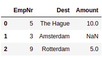
• Right outer join: In the right outer join, all the records from the right side of the DataFrame will be selected. If the matched records cannot be found in the left DataFrame, then it is filled with NaNs:

# Join DataFrames using Right Outer Join
df_right= pd.merge(dest, tips, on='EmpNr', how='right')
df_right.head()

This results in the following output:

• Left outer join: In the left outer join, all the records from the left side of the DataFrame will be selected. If the matched records cannot be found in the right DataFrame, then it is filled with NaNs:

# Join DataFrames using Left Outer Join
df_left= pd.merge(dest, tips, on='EmpNr', how='left')
df_left.head()

This results in the following output:

We will now move on to checking out missing values in the datasets.

Working with missing values

Most real-world datasets are messy and noisy. Due to their messiness and noise, lots of values are either faulty or missing. pandas offers lots of built-in functions to deal with missing values in DataFrames:

• Check missing values in a DataFrame: pandas' isnull() function checks for the existence of null values and returns True or False, where True is for null and False is for not-null values. The sum() function will sum all the True values and returns the count of missing values. We have tried two ways to count the missing values; both show the same output:

# Count missing values in DataFrame
pd.isnull(df).sum()

The following is the second method:

df.isnull().sum()

This results in the following output:

• Drop missing values: A very naive approach to deal with missing values is to drop them for analysis purposes. pandas has the dropna() function to drop or delete such observations from the DataFrame. Here, the inplace=True attribute makes the changes in the original DataFrame:

# Drop all the missing values
df.dropna(inplace=True)

df.info()

This results in the following output:

Here, the number of observations is reduced to 118 from 202.

• Fill the missing values: Another approach is to fill the missing values with zero, mean, median, or constant values:

# Fill missing values with 0
df.fillna(0,inplace=True)

df.info()

This results in the following output:

Here, we have filled the missing values with 0. This is all about handling missing values.

In the next section, we will focus on pivot tables.

Creating pivot tables

A pivot table is a summary table. It is the most popular concept in Excel. Most data analysts use it as a handy tool to summarize theire results. pandas offers the pivot_table() function to summarize DataFrames. A DataFrame is summarized using an aggregate function, such as mean, min, max, or sum. You can download the dataset from the following GitHub link: https://github.com/PacktPublishing/Python-Data-Analysis-Third-Edition/tree/master/Python-Data-Analysis-Third-Edition/Ch2:

# Import pandas
import pandas as pd

# Load data using read_csv()
purchase = pd.read_csv("purchase.csv")

# Show initial 10 records
purchase.head(10)

This results in the following output:

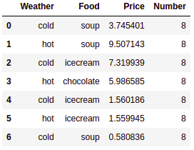
In the preceding code block, we have read the purchase.csv file using the read_csv() method.

Now, we will summarize the dataframe using the following code:

# Summarise dataframe using pivot table
pd.pivot_table(purchase,values='Number', index=['Weather',],
                    columns=['Food'], aggfunc=np.sum)

This results in the following output:

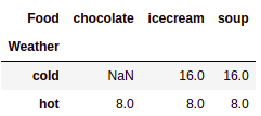
In the preceding example, the purchase DataFrame is summarized. Here, index is the Weather column, columns is the Food column, and values is the aggregated sum of the Number column. aggfun is initialized with the np.sum parameter. It's time to learn how to deal with dates in pandas DataFrames.

Dealing with dates

Dealing with dates is messy and complicated. You can recall the Y2K bug, the upcoming 2038 problem, and time zones dealing with different problems. In time-series datasets, we come across dates. pandas offers date ranges, resamples time-series data, and performs date arithmetic operations.

Create a range of dates starting from January 1, 2020, lasting for 45 days, as follows:

pd.date_range('01-01-2000', periods=45, freq='D')

Output:
DatetimeIndex(['2000-01-01', '2000-01-02', '2000-01-03', '2000-01-04',
               '2000-01-05', '2000-01-06', '2000-01-07', '2000-01-08',
               '2000-01-09', '2000-01-10', '2000-01-11', '2000-01-12',
               '2000-01-13', '2000-01-14', '2000-01-15', '2000-01-16',
               '2000-01-17', '2000-01-18', '2000-01-19', '2000-01-20',
               '2000-01-21', '2000-01-22', '2000-01-23', '2000-01-24',
               '2000-01-25', '2000-01-26', '2000-01-27', '2000-01-28',
               '2000-01-29', '2000-01-30', '2000-01-31', '2000-02-01',
               '2000-02-02', '2000-02-03', '2000-02-04', '2000-02-05',
               '2000-02-06', '2000-02-07', '2000-02-08', '2000-02-09',
               '2000-02-10', '2000-02-11', '2000-02-12', '2000-02-13',
               '2000-02-14'],
              dtype='datetime64[ns]', freq='D')

January has less than 45 days, so the end date falls in February, as you can check for yourself.

date_range() freq parameters can take values such as B for business day frequency, W for weekly frequency, H for hourly frequency, M for minute frequency, S for second frequency, L for millisecond frequency, and U for microsecond frequency. For more details, you can refer to the official documentation at https://pandas.pydata.org/pandas-docs/stable/user_guide/timeseries.html.

• pandas date range: The date_range() function generates sequences of date and time with a fixed-frequency interval:

# Date range function
pd.date_range('01-01-2000', periods=45, freq='D')

This results in the following output:

• to_datetime(): to_datetime() converts a timestamp string into datetime:

# Convert argument to datetime
pd.to_datetime('1/1/1970')

Output:  Timestamp('1970-01-01 00:00:00')

• We can convert a timestamp string into a datetime object in the specified format:

# Convert argument to datetime in specified format
pd.to_datetime(['20200101', '20200102'], format='%Y%m%d')

Output:
DatetimeIndex(['2020-01-01', '2020-01-02'], dtype='datetime64[ns]', freq=None)

• Handling an unknown format string: Unknown input format can cause value errors. We can handle this by using an errors parameter with coerce. coerce will set invalid strings to NaT:

# Value Error
pd.to_datetime(['20200101', 'not a date'])

Output:
ValueError: ('Unknown string format:', 'not a date')

# Handle value error
pd.to_datetime(['20200101', 'not a date'], errors='coerce')

Output:
DatetimeIndex(['2020-01-01', 'NaT'], dtype='datetime64[ns]', freq=None)

In the preceding example, the second date is still not valid and cannot be converted into a datetime object. The errors parameter helped us to handle such errors by inputting the value NaT (not a time).

Summary

In this chapter, we have explored the NumPy and pandas libraries. Both libraries help deal with arrays and DataFrames. NumPy arrays have the capability to deal with n-dimensional arrays. We have learned about various array properties and operations. Our main focus is on data types, data type as an object, reshaping, stacking, splitting, slicing, and indexing.

We also focused on the pandas library for Python data analysis. We saw how pandas mimics the relational database table functionality. It offers functionality to query, aggregate, manipulate, and join data efficiently.

NumPy and pandas work well together as a tool and make it possible to perform basic data analysis. At this point, you might be tempted to think that pandas is all we need for data analysis. However, there is more to data analysis than meets the eye.

Having picked up the fundamentals, it's time to proceed to data analysis with the commonly used statistics functions in Chapter 3, Statistics. This includes the usage of statistical concepts.

You are encouraged to read the books mentioned in the References section for exploring NumPy and pandas in further detail and depth.

References

• Ivan Idris, NumPy Cookbook – Second Edition, Packt Publishing, 2015.
• Ivan Idris, Learning NumPy Array, Packt Publishing, 2014.
• Ivan Idris, NumPy: Beginner's Guide – Third Edition, Packt Publishing, 2015.
• L. (L.-H.) Chin and T. Dutta, NumPy Essentials, Packt Publishing, 2016.
• T. Petrou, Pandas Cookbook, Packt Publishing, 2017.
• F. Anthony, Mastering pandas, Packt Publishing, 2015.
• M. Heydt, Mastering pandas for Finance, Packt Publishing, 2015.
• T. Hauck, Data-Intensive Apps with pandas How-to, Packt Publishing, 2013.
• M. Heydt, Learning pandas, Packt Publishing, 2015.