
PROJECT
![]()
Predicting Used Car Sale Price Using Feedforward Artificial Neural Networks
In project 1 of this book, you saw how we can predict the sale prices of houses using linear regression. In this article, you will see how we can use a feedforward artificial neural network to predict the prices of used cars. The car sale price prediction problem is a regression problem like house price prediction since the price of a car is a continuous value.
In this project, you will see how to predict car sale prices using a densely connected neural network (DNN), which is a type of feedforward neural network. Though you can implement a densely connected neural network from scratch in Python, in this project, you will be using the TensorFlow Keras library to implement a feedforward neural network.
What is a FeedForward DNN?
A feedforward densely connected neural network (DNN) is a type of neural network where all the nodes in the previous layer are connected to all the nodes in the subsequent layer of a neural network. A DNN is also called a multilayer perceptron.
A densely connected neural network is mostly used for making predictions on tabular data. Tabular data is the type of data that can be presented in the form of a table.
In a neural network, we have an input layer, one or multiple hidden layers, and an output layer. An example of a neural network is shown below:

In our neural network, we have two nodes in the input layer (since there are two features in the input), one hidden layer with four nodes, and one output layer with one node since we are doing binary classification. The number of hidden layers and the number of neurons per hidden layer depend upon you.
In the above neural network, x1 and x2 are the input features, and ao is the output of the network. Here, the only thing we can control is the weights w1, w2, w3, … w12. The idea is to find the values of weights for which the difference between the predicted output, ao, in this case, and the actual output (labels).
A neural network works in two steps:
1.FeedForward
2.BackPropagation
I will explain both these steps in the context of our neural network.
FeedForward
In the feedforward step, the final output of a neural network is created. Let’s try to find the final output of our neural network.
In our neural network, we will first find the value of zh1, which can be calculated as follows:
![]()
Using zh1, we can find the value of ah1, which is:
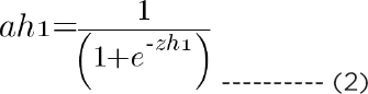
In the same way, you find the values of ah2, ah3, and ah4.
To find the value of zo, you can use the following formula:
![]()
Finally, to find the output of the neural network ao:

Backpropagation
The purpose of backpropagation is to minimize the overall loss by finding the optimum values of weights. The loss function we are going to use in this section is the mean squared error, which is, in our case, represented as:

Here, ao is the predicted output from our neural network, and y is the actual output.
Our weights are divided into two parts. We have weights that connect input features to the hidden layer and the hidden layer to the output node. We call the weights that connect the input to the hidden layer collectively as wh (w1, w2, w3 … w8), and the weights connecting the hidden layer to the output as wo (w9, w10, w11, and w12).
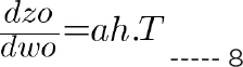
The backpropagation will consist of two phases. In the first phase, we will find dcost/dwo (which refers to the derivative of the total cost with respect to wo (weights in the output layer)). By the chain rule, dcost/dwo can be represented as the product of dcost/dao * dao/dzo * dzo/dwo (d here refers to derivative). Mathematically:
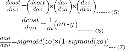
In the same way, you find the derivative of cost with respect to bias in the output layer, i.e., dcost/dbo, which is given as:

Putting 6, 7, and 8 in equation 5, we can get the derivative of cost with respect to the output weights.
The next step is to find the derivative of cost with respect to hidden layer weights, wh, and bias, bh. Let’s first find the derivative of cost with respect to hidden layer weights:

The values of dcost/dao and dao/dzo can be calculated from equations 6 and 7, respectively. The value of dzo/dah is given as:

Putting the values of equations 6, 7, and 8 in equation 11, you can get the value of equation 10.
Next, let’s find the value of dah/dzh:
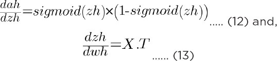
Using equation 10, 12, and 13 in equation 9, you can find the value of dcost/dwh.
Why Use a Linear Feedforward DNN?
A Feedforward DNN has the following advantages:
1.Neural networks produce better results compared to traditional algorithms when you have a large amount of training data.
2.Neural networks are capable of finding hidden features from data that are otherwise not visible to the human eye.
Disadvantages of Feedforward DNN
Following are the disadvantages of neural networks:
1.Require a large amount of training data to produce good results.
2.It can be slow during training time if you have a large number of layers and nodes in your neural network.
In the next steps, you will see how we can create a feedforward densely connected neural network with the TensorFlow Keras library.
3.1. Installing the Required Libraries
If you run the scripts on Google Colab (https://colab.research.google.com/), you do not need to install any library. All the libraries are preinstalled on Google Colab. On the other hand, if you want to run the scripts in this section on your local system or any remote server, you will need to install the following libraries:
$pip install scikit-learn
$pip install numpy
$pip install pandas
$pip install matplotlib
$pip install seaborn
You also need to install TensorFlow 2.0 to run the scripts. The instructions to download TensorFlow 2.0 are available on their official blog.
3.2. Importing the Libraries
The second step is to import the required libraries. Execute the following script to do so:
Script 1:
import pandas as pd
import numpy as np
import matplotlib.pyplot as plt
from sklearn.model_selection import train_test_split
%matplotlib inline
import seaborn as sns
sns.set(style=”darkgrid”)
import tensorflow as tf
print(tf.__version__)
3.3. Importing the Dataset
The dataset that we are going to use to train our feedforward neural network for predicting car sale price can be downloaded from this Kaggle link: https://bit.ly/37E1Ktg. From the above link, download the train.csv file only.
The dataset is also available by the name: car_data.csv in the Datasets folder in the GitHub and SharePoint repositories. Download the dataset to your local file system, and use the read_csv() method of the Pandas library to read the dataset into a Pandas dataframe, as shown in the following script. The following script also prints the first five rows of the dataset using the head() method.
Script 2:
1. data_path = r”/content/car_data.csv”
2. car_dataset = pd.read_csv(data_path, engine=’python’)
3. car_dataset.head()
Output:

3.4. Data Visualization and Preprocessing
Let’s first see the percentage of the missing data in all the columns. The following script does that.
Script 3:
1. car_dataset.isnull().mean()
Output:
| Unnamed: 0 | 0.000000 |
| Name | 0.000000 |
| Location | 0.000000 |
| Year | 0.000000 |
| Kilometers_Driven | 0.000000 |
| Fuel_Type | 0.000000 |
| Transmission | 0.000000 |
| Owner_Type | 0.000000 |
| Mileage | 0.000332 |
| Engine | 0.005981 |
| Power | 0.005981 |
| Seats | 0.006978 |
| New_Price | 0.863100 |
| Price | 0.000000 |
| dtype: float64 |
The output above shows that the Mileage, Engine, Power, Seats, and New_Price column contains missing values. The highest percentage of missing values is 86.31 percent, which belongs to the New_Price column. We will remove the New_Price column. Also, the first column, i.e., “Unnamed: 0” doesn’t convey any useful information. Therefore, we will delete that column, too. The following script deletes these two columns.
Script 4:
1. car_dataset = car_dataset.drop([‘Unnamed: 0’, ‘New_Price’], axis = 1)
We will be predicting the value in the Price column of the dataset. Let’s plot a heatmap that shows a relationship between all the numerical columns in the dataset.
Script 5:
1. plt.rcParams[“figure.figsize”] = [8, 6]
2. sns.heatmap(car_dataset.corr())
Output:

The output shows that there is a very slight positive correlation between the Year and the Price columns, which makes sense as newer cars are normally expensive compared to older cars.
Let’s now plot a histogram for the Price to see the price distribution.
Script 6:
1. sns.distplot(car_dataset[‘Price’])
Output:

The output shows that most of the cars are priced between 2.5 to 7.5 hundred thousand. Remember, the unit of the price mentioned in the price column is one hundred thousand.
3.5. Converting Categorical Columns to Numerical
Our dataset contains categorical values. Neural networks work with numbers. Therefore, we need to convert the values in the categorical columns to numbers.
Let’s first see the number of unique values in different columns of the dataset.
Script 7:
1. car_dataset.nunique()
Output:
| Name | 1876 |
| Location | 11 |
| Year | 22 |
| Kilometers_Driven | 3093 |
| Fuel_Type | 5 |
| Transmission | 2 |
| Owner_Type | 4 |
| Mileage | 442 |
| Engine | 146 |
| Power | 372 |
| Seats | 9 |
| Price | 1373 |
| dtype: int64 |
Next, we will print the data types of all the columns.
Script 8:
1. print(car_dataset.dtypes)
Output:
| Name | object |
| Location | object |
| Year | int64 |
| Kilometers_Driven | int64 |
| Fuel_Type | object |
| Transmission | object |
| Owner_Type | object |
| Mileage | object |
| Engine | object |
| Power | object |
| Seats | float64 |
| Price | float64 |
| dtype: object |
From the above output, the columns with object type are the categorical columns. We need to convert these columns into a numeric type.
Also, the number of unique values in the Name column is too large. Therefore, it might not convey any information for classification. Hence, we will remove the Name column from our dataset.
We will follow a step by step approach. First, we will separate numerical columns from categorical columns. Then, we will convert categorical columns into one-hot categorical columns, and, finally, we will merge the one-hot encoded columns with the original numerical columns. The process of one-hot encoding is explained in a later section.
The following script creates a dataframe of numerical columns only by removing all the categorical columns from the dataset.
Script 9:
1. numerical_data = car_dataset.drop([‘Name’, ‘Location’, ‘Fuel_Type’, ‘Transmission’, ‘Owner_Type’, ‘Mileage’, ’Engine’, ‘Power’], axis=1)
2. numerical_data.head()
In the following output, you can see only the numerical columns in our dataset.
Output

Next, we will create a dataframe of categorical columns only by filtering all the categorical columns (except Name, since we want to drop it) from the dataset. Look at the following script for reference.
Script 10:
1. categorical_data = car_dataset.filter([‘Location’, ‘Fuel_Type’, ‘Transmission’, ‘Owner_Type’, ‘Mileage’, ’Engine’, ‘Power’], axis=1)
2. categorical_data.head()
The output below shows a list of all the categorical columns:
Output:

Now, we need to convert the categorical_data dataframe, which contains categorical values, into numeric form.
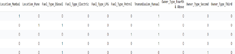
One of the most common approaches to convert a categorical column to a numeric one is via one-hot encoding. In one-hot encoding, for every unique value in the original columns, a new column is created. For instance, since the number of unique values in the categorical Transmission column is two, i.e., Manual and Transmission, for the Transmission categorical column in our dataset, two new numeric columns: Transmission_Manual and Transmission_Automatic will be created. If the original Transmission column contained the value Manual, 1 is added in the newly created Transmission_Manual column, while 0 is added in the Transmission_Automatic column.
However, it can be noted that we do not really need two columns. A single column, i.e., Transmission_Manual is enough since when the Transmission is Manual, we can add 1 in the Transmission_Manual column, else 0 can be added in that column. Hence, we actually need N-1 one-hot encoded columns for all the N unique values in the original column.
The following script converts categorical columns into one-hot encoded columns using the pd.get_dummies() method.
Script 11:
1. categorical_data__one_hot = pd.get_dummies(categorical_data, drop_first= True)
2. categorical_data__one_hot.head()
A snapshot of the one-hot encoded columns is shown below.
Output:
Finally, the following script concatenates the numerical columns with one-hot encoded columns to create a final dataset.
Script 12:
1. complete_dataset = pd.concat([numerical_data, categorical_data__one_hot], axis=1)
2. complete_dataset.head()
Here is the output:
Output:

Before dividing the data into training and test sets, we will again check if our data contains null values.
Script 13:
1. complete_dataset.isnull().mean()
Output:
| Year | 0.000000 |
| Kilometers_Driven | 0.000000 |
| Seats | 0.006978 |
| Price | 0.000000 |
| Location_Bangalore | 0.000000 |
| … | |
| Power_98.82 bhp | 0.000000 |
| Power_98.96 bhp | 0.000000 |
| Power_99 bhp | 0.000000 |
| Power_99.6 bhp | 0.000000 |
| Power_null bhp | 0.000000 |
| Length: 979, dtype: float64 |
Now, instead of removing columns, we can remove the rows that contain any null values. To do so, execute the following script:
Script 14:
1. complete_dataset.dropna(inplace = True)
Before we train our neural network, we need to divide the data into training and test sets, as we did for project 1 and project 2.
3.6. Dividing Data into Training and Test Sets
The following script divides the data into features and labels sets. The Feature set (X in this Project) consists of all the columns except the Price column from the complete_dataset dataframe, while the label set (y in this project) contains the values from the Price column.
Script 15:
1. X = complete_dataset.drop([‘Price’], axis=1)
2. y = complete_dataset[‘Price’]
Like traditional machine learning algorithms, neural networks are trained on the training set and are evaluated on the test set. Therefore, we need to divide our dataset into the training and test sets, as shown below:
Script 16:
1. X_train, X_test, y_train, y_test = train_test_split(X, y, test_size=0.20, random_state=20)
To train neural networks, it is always a good approach to scale your feature set. The following script can be used for feature scaling of training and test features.
Script 17:
1. from sklearn.preprocessing import StandardScaler
2. scaler = StandardScaler()
3. X_train = scaler.fit_transform(X_train)
4. X_test = scaler.transform(X_test)
3.7. Creating and Training Neural Network Model with Tensor Flow Keras
Now, we are ready to create our neural network in TensorFlow Keras. First, import the following modules and classes.
Script 18:
1. from tensorflow.keras.layers import Input, Dense, Activation,Dropout
2. from tensorflow.keras.models import Model
The following script describes our neural network. To train a feedforward neural network on tabular data using Keras, you have to first define the input layer using the Input class. The shape of the input in case of tabular data, such as the one we have, should be (Number of Features). The shape is specified by the shape attribute of the Input class.
Next, you can add as many dense layers as you want. In the following script, we add six dense layers with 100, 50, 25, 10, 5, and 2 nodes. Each dense layer uses the relu activation function. The input to the first dense layer is the output from the input layer. The input to each layer is specified in a round bracket that follows the layer name. The output layer in the following script also consists of a dense layer but with 1 node since we are predicting a single value.
Script 19:
1. input_layer = Input(shape=(X.shape[1],))
2. dense_layer0 = Dense(100, activation=’relu’)(input_layer)
3. dense_layer1 = Dense(50, activation=’relu’)(dense_layer0)
4. dense_layer2 = Dense(25, activation=’relu’)(dense_layer1)
5. dense_layer3 = Dense(10, activation=’relu’)(dense_layer2)
6. dense_layer4 = Dense(5, activation=’relu’)(dense_layer3)
7. dense_layer5 = Dense(2, activation=’relu’)(dense_layer4)
8. output = Dense(1)(dense_layer5)
The previous script described the layers. Now is the time to develop the model. To create a neural network model, you can use the Model class from tensorflow.keras.models module, as shown in the following script. The input layer is passed to the inputs attribute, while the output layer is passed to the outputs module.
To compile the model, you need to call the compile() method of the model and then specify the loss function, the optimizer, and the metrics. Our loss function is “mean_absolute_error,” “optimizer” is adam, and metrics is also the mean absolute error since we are evaluating a regression problem. To study more about Keras optimizers, check this link: https://keras.io/api/optimizers/. And to study more about loss functions, check this link: https://keras.io/api/losses/.
Script 20:
1. model = Model(inputs = input_layer, outputs=output)
2. model.compile(loss=”mean_absolute_error”, optimizer=”adam”, metrics=[“mean_absolute_error”])
You can also plot and see how your model looks using the following script:
Script 21:
1. from keras.utils import plot_model
2. plot_model(model, to_file=’model_plot.png’, show_shapes=True, show_layer_names=True)
You can see all the layers and the number of inputs and outputs from the layers, as shown below:
Output:


Finally, to train the model, you need to call the fit() method of model class and pass it your training features and test features. Twenty percent of the data from the training set will be used as validation data, while the algorithm will be trained five times on the complete dataset five, as shown by the epochs attribute. The batch size will also be 5.
Script 22:
1. history = model.fit(X_train, y_train, batch_size=5, epochs=5, verbose=1, validation_split=0.2)
The five epochs are displayed below:
Output:

3.8. Evaluating the Performance of a Neural Network Model
After the model is trained, the next step is to evaluate model performance. There are several ways to do that. One of the ways is to plot the training and test loss, as shown below:
Script 23:
1. plt.plot(history.history[‘loss’])
2. plt.plot(history.history[‘val_loss’])
3.
4. plt.title(‘loss’)
5. plt.ylabel(‘loss’)
6. plt.xlabel(‘epoch’)
7. plt.legend([‘train’,’test’], loc=’upper left’)
8. plt.show()
Output:

The above output shows that while the training loss keeps decreasing till the fifth epoch, the test or validation loss shows fluctuation after the second epoch, which shows that our model is slightly overfitting.
Another way to evaluate is to make predictions on the test set and then use regression metrics such as MAE, MSE, and RMSE to evaluate model performance.
To make predictions, you can use the predict() method of the model class and pass it the test set, as shown below:
Script 24:
1. y_pred = model.predict(X_test)
The following script calculates the values for MAE, MSE, and RMSE on the test set.
Script 25:
1. from sklearn import metrics
2.
3. print(‘Mean Absolute Error:’, metrics.mean_absolute_error(y_test, y_pred))
4. print(‘Mean Squared Error:’, metrics.mean_squared_error(y_test, y_pred))
5. print(‘Root Mean Squared Error:’, np.sqrt(metrics.mean_squared_error(y_test, y_pred)))
Output:
Mean Absolute Error: 1.869464170857018
Mean Squared Error: 22.80469457178821
Root Mean Squared Error: 4.775426114158632
The above output shows that we have a mean error of 1.86. The mean of the Price column can be calculated as follows:
Script 26:
1. car_dataset[‘Price’].mean()
Output:
9.479468350224273
We can find the mean percentage error by dividing MAE by the average of the Price column, i.e., 1.86/9.47 = 0.196. The value shows that, on average, for all the cars in the test set, the prices predicted by our feedforward neural network and the actual prices differ by 19.6 percent.
You can plot the actual and predicted prices side by side, as follows:
Script 27:
1. comparison_df = pd.DataFrame({‘Actual’: y_test.values.tolist(), ‘Predicted’: y_pred.tolist()})
2. comparison_df
Output:

3.9. Making Predictions on a Single Data Point
In this section, you will see how to make predictions for a single car price. Let’s print the shape of the feature vector or record at the first index in the test set.
Script 28:
1. X_test[1].shape
From the output below, you can see that this single record has one dimension.
Output:
(978,)
As we did in project 1, to make predictions on a single record, the feature vector for the record should be in the form of a row vector. You can covert the feature vector for a single record into the row vector using the reshape(1,–1) method, as shown below:
Script 29:
1. single_point = X_test[1].reshape(1,-1)
2. single_point.shape
Output:
(1, 978)
The output shows that the shape of the feature has now been updated to a row vector.
To make predictions, you simply have to pass the row feature vector to the predict() method of the trained neural network model, as shown below:
Script 30:
1. model.predict(X_test[1].reshape(1,-1))
The predicted price is 5.06 hundred thousand.
Output:
array([[5.0670004]], dtype=float32)
The actual price can be printed via the following script:
Script 31:
y_test.values[1]
Output:
5.08
The actual output is 5.08 hundred thousand, which is very close to the 5.06 hundred thousand predicted by our model. You can take any other record from the test set, make a prediction on that using the trained neural network, and see how close you get.
| Further Readings – TensorFlow Keras Neural Networks |
| To know more about neural networks in TensorFlow Keras, check out these links: https://keras.io/ https://www.tensorflow.org/tutorials/keras/regression |
Exercise 3.1
Question 1:
In a neural network with three input features, one hidden layer of 5 nodes, and an output layer with three possible values, what will be the dimensions of weight that connects the input to the hidden layer? Remember, the dimensions of the input data are (m,3), where m is the number of records.
A.[5,3]
B.[3,5]
C.[4,5]
D.[5,4]
Question 2:
Which of the following loss functions can you use in case of regression problems?
A.Sigmoid
B.Negative log likelihood
C.Mean Absolute Error
D.Softmax
Question 3:
Neural networks with hidden layers are capable of finding:
A.Linear boundaries
B.Non-linear boundaries
C.All of the above
D.None of the above