PROJECT

Classifying Cats and Dogs Images Using Convolutional Neural Networks

In the previous three projects, you studied different feedforward densely connected neural networks and recurrent neural networks. In this project, you will study the Convolutional Neural Network (CNN).

You will see how you can use convolutional neural networks (CNN) to classify cats’ and dogs’ images. Before you see the actual code, let’s first briefly discuss what convolutional neural networks are.

What Is a Convolutional Neural Network?

A convolutional neural network, a type of neural network, is used to classify spatial data, for instance, images, sequences, etc. In an image, each pixel is somehow related to some other pictures. Looking at a single pixel, you cannot guess the image. Rather, you have to look at the complete picture to guess the image. A CNN does exactly that. Using a kernel or feature detects, it detects features within an image.

A combination of these images then forms the complete image, which can then be classified using a densely connected neural network. The steps involved in a Convolutional Neural Network have been explained in the next section.

6.1. How CNN Classifies Images?

Before we actually implement a CNN with TensorFlow Keras library for cats and dogs’ image classification, let’s briefly see how a CNN classifies images.

How Do Computers See Images?

When humans see an image, they see lines, circles, squares, and different shapes. However, a computer sees an image differently. For a computer, an image is no more than a 2-D set of pixels arranged in a certain manner. For greyscale images, the pixel value can be between 0–255, while for color images, there are three channels: red, green, and blue. Each channel can have a pixel value between 0–255.

Look at the following image 6.1.

Image 6.1: How do computers see images?

Here, the box on the leftmost is what humans see. They see a smiling face. However, a computer sees it in the form of pixel values of 0s and 1s, as shown on the right-hand side. Here, 0 indicates a white pixel, whereas 1 indicates a black pixel. In the real world, 1 indicates a white pixel, while 0 indicates a black pixel.

Now, we know how a computer sees images, the next step is to explain the steps involved in the image classification using a convolutional neural network.

The following are the steps involved in image classification with CNN:

1.The Convolution Operation

2.The ReLu Operation

3.The Pooling Operation

4.Flattening and Fully Connected Layer

The Convolution Operation

The convolution operation is the first step involved in the image classification with a convolutional neural network.

In convolution operation, you have an image and a feature detector. The values of the feature detector are initialized randomly. The feature detector is moved over the image from left to right. The values in the feature detector are multiplied by the corresponding values in the image, and then all the values in the feature detector are added. The resultant value is added to the feature map.

Look at the following image, for example:

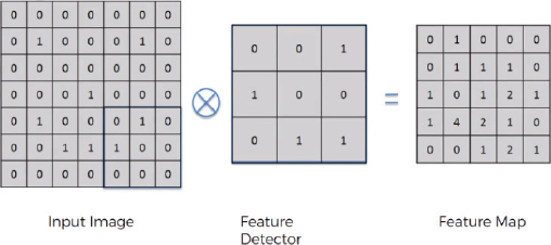
In the above figure, we have an input image of 7 x 7. The feature detector is of size 3 x 3. The feature detector is placed over the image at the top left of the input image, and then the pixel values in the feature detector are multiplied by the pixel values in the input image. The result is then added. The feature detector then moves to the N step toward the right. Here, N refers to stride. A stride is basically the number of steps that a feature detector takes from left to right and then from top to bottom to find a new value for the feature map.

In reality, there are multiple feature detectors, as shown in the following image:

Each feature detector is responsible for detecting a particular feature in the image.

The ReLu Operation

In the ReLu operation, you simply apply the ReLu activation function on the feature map generated as a result of the convolution operation. Convolution operation gives us linear values. The ReLu operation is performed to introduce non-linearity in the image.

In the ReLu operation, all the negative values in a feature map are replaced by 0. All the positive values are left untouched.

Suppose we have the following feature map:

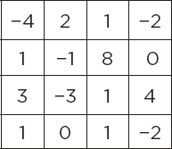
When the ReLu function is applied on the feature map, the resultant feature map looks like this:

The Pooling Operation

Pooling operation is performed in order to introduce spatial invariance in the feature map. Pooling operation is performed after convolution and ReLu operations.

Let’s first understand what spatial invariance is. If you look at the following three images, you can easily identify that these images contain cheetahs.

The second image is disoriented, and the third image is distorted. However, we are still able to identify that all three images contain cheetahs based on certain features.

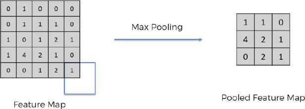
Pooling does exactly that. In pooling, we have a feature map and then a pooling filter, which can be of any size. Next, we move the pooling filter over the feature map and apply the pooling operation. There can be many pooling operations, such as max pooling, min pooling, and average pooling. In max pooling, we choose the maximum value from the pooling filter. Pooling not only introduces spatial invariance but also reduces the size of an image.

Look at the following image. Here, in the 3^rd and 4^th rows and 1^st and 2^nd columns, we have four values 1, 0, 1, and 4. When we apply max pooling on these four pixels, the maximum value will be chosen, i.e., you can see 4 in the pooled feature map.

Flattening and Fully Connected Layer

For finding more features from an image, the pooled feature maps are flattened to form a one-dimensional vector, as shown in the following figure:

The one-dimensional vector is then used as input to the densely or fully connected neural network layer that you saw in project 3. This is shown in the following image:

6.2. Cats and Dogs Image Classification with a CNN

In this section, we will move forward with the implementation of the convolutional neural network in Python. We know that a convolutional neural network can learn to identify the related features on a 2D map, such as images. In this project, we will solve the image classification task with CNN. Given a set of images, the task is to predict whether an image contains a cat or a dog.

Importing the Dataset and Required Libraries

The dataset for this project consists of images of cats and dogs. The dataset can be downloaded directly from this Kaggle Link (https://www.kaggle.com/c/dogs-vs-cats).

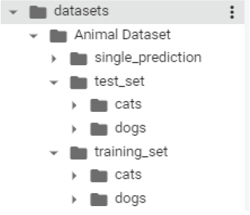
The dataset is also available inside the Animal Datasets, which is located inside the Datasets folder in the GitHub and SharePoint repositories. The original dataset consists of 2,500 images. But the dataset that we are going to use will be smaller and will consist of 10,000 images. Out of 10,000 images, 8,000 images are used for training, while 2,000 images are used for testing. The training set consists of 4,000 images of cats and 4,000 images of dogs. The test set also contains an equal number of images of cats and dogs.

It is important to mention that the dataset should be arranged in the following directory structure for TensorFlow Keras to extract images and their corresponding labels:

As a first step, upgrade to the latest version of the TensorFlow library.

Script 1:

The image dataset in this project is uploaded to Google Drive so that it can be accessed easily by the Google collaborator environment. The following script will mount your Google Drive in your Google Collaborator environment.

Script 2:

Let’s import the TensorFlow Keras libraries necessary to create a convolutional neural network.

Script 3:

6.2.1. Creating Model Architecture

In the previous two projects, we used the Keras Functional API to create the TensorFlow Keras model. The Functional API is good when you have to develop complex deep learning models. For simpler deep learning models, you can use Sequential API, as well. In this project, we will build our CNN model using sequential API.

To create a sequential model, you have to first create an object of the Sequential class from the tensorflow.keras.models module.

Script 4:

Next, you can create layers and add them to the Sequential model object that you just created.

The following script adds a convolution layer with 32 filters of shape 3 x 3 to the sequential model. Notice that the input shape size here is 64, 64, 3. This is because we will resize our images to a pixel size of 64 x 64 before training. The dimension 3 is added because a color image has three channels, i.e., red, green, and blue (RGB).

Script 5:

Next, we will create a pooling layer of size 2, 2, and add it to our sequential CNN model, as shown below.

Script 6:

Let’s add one more convolution and one more pooling layer to our sequential model. Look at scripts 7 and 8 for reference.

Script 7:

Script 8:

You can add more convolutional and sequential layers if you want.

As you studied in the theory section, the convolutional and pooling layers are followed by dense layers. To connect the output of convolutional and pooling layers to dense layers, you need to flatten the output first using the Flatten layer, as shown below.

Script 9:

We add two dense layers to our model. The first layer will have 128 neurons, and the second dense layer, which will also be the output layer, will consist of 1 neuron since we are predicting a single value. Scripts 10 and 11, shown below, add the final two dense layers to our model.

Script 10:

Script 11:

As we did in the previous project, before training a model, we need to compile it. To do so, you can use the compile model, as shown below. The optimizer we used is adam, whereas the loss function is binary_cross entropy since we have only two possible outputs, i.e., whether an image can be a cat or a dog.

And since this is a classification problem, the performance metric has been set to ‘accuracy’.

Script 12:

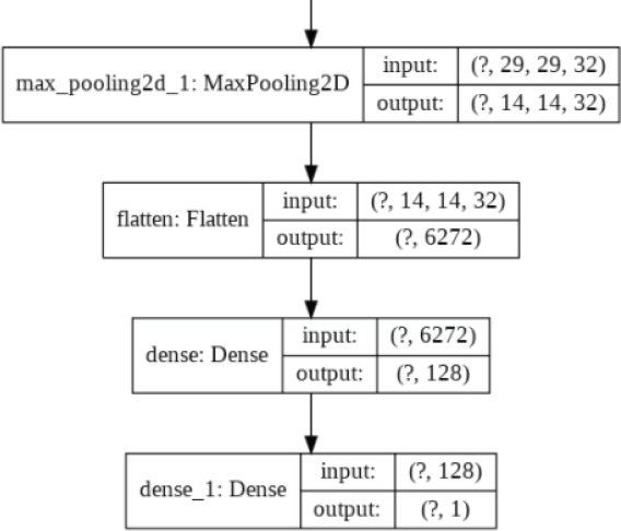
Let’s plot our model to see its overall architecture:

Script 13:

Output:

6.2.2. Image Augmentation

To improve the image and to increase the image uniformity, you can apply several preprocessing steps to an image. To do so, you can use the ImageDataGenerator class from the tensorflow.keras.preprocessing.image module. The following script applies feature scaling to the training and test images by dividing each pixel value by 255. Next, a shear value and zoom range of 0.2 is also added to the image. Finally, all the images are flipped horizontally.

To know more about ImageDataGenerator class, take a look at this official documentation link: https://keras.io/api/preprocessing/image/.

The following script applies image augmentation to the training set.

Script 14:

And the following script applies image augmentation to the test set. Note that we only apply feature scaling to the test set, and no other preprocessing step is applied to the test set.

Script 15:

6.2.3. Dividing Data into Training & Test Sets

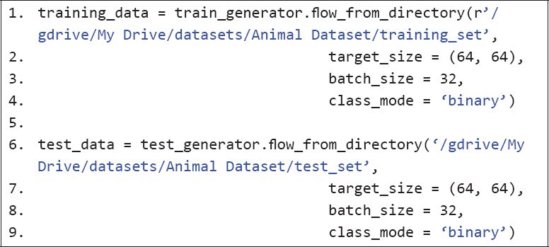
Next, we need to divide the data into training and test sets. Since the images are in a local directory, you can use the flow_from_directory() method of the ImageDataGenerator object for the training and test sets.

You need to specify the target size (image size), which is 64, 64 in our case. The batch size defines the number of images that will be processed in a batch. And finally, since we have two output classes for our dataset, the class_mode attribute is set to binary.

The following script creates the final training and test sets.

Script 16:

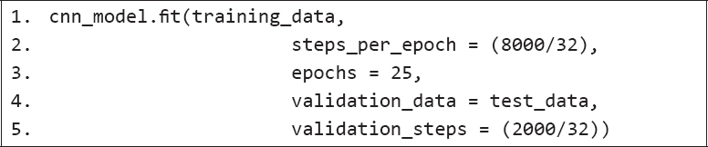
6.2.4. Training a CNN Model

Training the model is easy. You just need to pass the training and test sets to the fit() method of your CNN model. You need to specify the steps per epoch. Steps per epoch refers to the number of times you want to update the weights of your neural network in one epoch. Since we have 8,000 records in the training set where 32 images are processed in a bath, the steps per epoch will be 8000/32 = 250. Similarly, in the test set, we process 32 images at a time. The validation step is also set to 2000/32, which means that the model will be validated on the test set after a batch of 32 images.

Script 17:

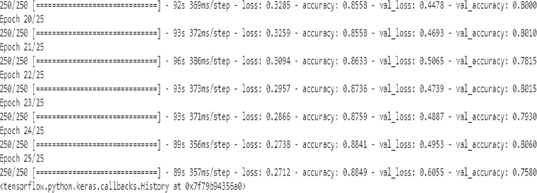
The output after 25 epochs is as follows. An accuracy of 88.49 percent is achieved on the training set, while an accuracy of 75.80 is achieved on the test set.

Output:

6.2.5. Making Prediction on a Single Image

Let’s now see how you can make predictions on a single image. If you look at the single_prediction folder in your dataset, it contains two images: cat_or_dog_1.jpg and cat_or_dog2.jpg. We will be predicting what is in the first image, i.e., cat_or_dog1.jpg.

Execute the following script to load the cat_or_dog1.jpg image and convert it into an image of 64 x 64 pixels.

Script 18:

Let’s look at the image type.

Script 19:

Output:

The image type is PIL. We need to convert it into array type so that our trained CNN model can make predictions on it. To do so, you can use the img_to_array() function of the image from the tensorflow.keras.preprocessing module, as shown below.

Script 20:

The above script also adds one extra dimension to the image array because the trained model is trained using an extra dimension, i.e., batch. Therefore, while making a prediction, you also need to add the dimension for the batch. Though the batch size for a single image will always be 1, you still need to add the dimension in order to make a prediction.

Finally, to make predictions, you need to pass the array for the image to the predict() method of the CNN model, as shown below:

Script 21:

The prediction made by a CNN model for binary classification will be 0 or 1. To check the index values for 0 and 1, you can use the following script.

Script 22:

The following output shows that 0 corresponds to a cat while 1 corresponds to a dog.

Output:

Let’s print the value of the predicted result. To print the value, you need to first specify the batch number and image number. Since you have only one batch and only one image within that batch, you can specify 0 and 0 for both.

Script 23:

Output:

The output depicts a value of 1.0, which shows that the predicted image contains a dog. To verify, open the image Animal Dataset/single_prediction/cat_or_dog_1.jpg, and you should see that it actually contains an image of a dog, as shown below. This means our prediction is correct!

Further Readings – Image Classification with CNN

To study more about image classification with TensorFlow Keras, take a look at these links: https://bit.ly/3ed8PCg https://bit.ly/2TFijwU

Exercise 6.1

Question 1

What should be the input shape of the input image to the convolutional neural network?

A.Width, Height

B.Height, Width

C.Channels, Width, Height

D.Width, Height, Channels

Question 2

The pooling layer is used to pick correct features even if:

A.Image is inverted

B.Image is distorted

C.Image is compressed

D.All of the above

Question 3

The ReLu activation function is used to introduce:

A.Linearity

B.Non-linearity

C.Quadraticity

D.None of the above