Centralized Logging

Logging follows close behind automation in importance. In large-scale, distributed systems, logging isn’t optional. Special attention must be paid to logging at both the application level and the environment level.

For example, exceptions should always be sent to the centralized logging system. On the other hand, while developing software, it is often a good idea to create debug logging instead of print statements. Why do this? Many hours are spent developing heuristics to debug the source code. Why not capture that so it can be turned on if a problem surfaces in production again?

The trick here is logging levels. By creating debug log levels that only appear in the nonproduction environment, it allows the logic of debugging to be kept in the source code. Likewise, instead of having overly verbose logs appear in production and add confusion, they can be toggled on and off.

An example of logging in large-scale distributed systems is what Ceph uses: daemons can have up to 20 debug levels! All of these levels are handled in code, allowing the system to fine-tune the amount of logging. Ceph furthers this strategy by being able to restrict the amount of logging per daemon. The system has a few daemons, and the logging can be increased for one or all of them.

Case Study: Production Database Kills Hard Drives

Another vital strategy for logging is solving scalability. Once the application is large enough, it might not be feasible to store all logs in a file anymore. Alfredo was once tasked to debug a problem with the primary database of an extensive web application that hosted about one hundred newspaper, radio station, and television station sites. These sites generated lots of traffic and produced massive amounts of logs. So much log output was created that the logging for PostgreSQL was set to a minimum, and he couldn’t debug the problem because it required raising the log level. If the log level was raised, the application would stop working from the intense I/O generated. Every day at around five o’clock in the morning, the database load spiked. It had gotten progressively worse.

The database administrators were opposed to raising the log levels to see the most expensive queries (PostgreSQL can include query information in the logs) for a whole day, so we compromised: fifteen minutes at around five o’clock in the morning. As soon as he was able to get those logs, Alfredo immediately got to rate the slowest queries and how often they were run. There was a clear winner: a SELECT * query that was taking so long to complete that the fifteen-minute window was not enough to capture its runtime. The application didn’t do any queries that selected everything from any table; what could it be?

After much persuasion, we got access to the database server. If the spike in load happens at around five o’clock in the morning every single day, is it possible that there is some recurrent script? We looked into crontab (the program that keeps track of what runs at given intervals), which showed a suspicious script: backup.sh. The contents of the script had a few SQL statements that included several SELECT *. The database administrators were using this to back up the primary database, and as the size of the database grew, so did the load until it was no longer tolerable. The solution? Stop using the script, and back up one of the four secondary (replica) databases.

That saved the backup problem, but it didn’t help the inability to have access to logs. Thinking ahead on distributing logging output is the right approach. Tools like rsyslog are meant to solve this, and if added from the start, it can save you from being unable to solve a production outage.

Did You Build It or Buy It?

It is incredible how much vendor lock-in gets press. Vendor lock-in, though, is in the eye of the beholder. You can pretty much throw a rock in any direction in downtown San Francisco and hit someone preaching the evils of vendor lock-in. When you dig a little deeper though, you wonder what their alternative is.

In Economics, there is a principle called comparative advantage. In a nutshell, it means there is an economic benefit to focusing on what you are best at and outsourcing other tasks to other people. With the cloud, in particular, there is continuous improvement, and end-users benefit from that improvement without an aggregated cost—and most of the time with less complexity than before.

Unless your company is operating at the scale of one of the giants in technology, there is almost no way to implement, maintain, and improve a private cloud and be able to save money and improve the business at the same time. For example, in 2017, Amazon released the ability to deploy multimaster databases with automatic failover across multiple Availability Zones. As someone who has attempted this, I can say that it is borderline impossible and tremendously hard to add the ability of automatic failover in such a scenario. One of the golden questions to consider regarding outsourcing is: “Is this a core competency of the business?” A company that runs its own mail server but its core competency is selling car parts is playing with fire and probably already losing money.

Fault Tolerance

Fault tolerance is a fascinating topic but it can be very confusing. What is meant by fault tolerance, and how can you achieve it? A great place to learn more about fault tolerance is to read as many white papers from AWS as you can.

When designing fault-tolerant systems, it’s useful to start by trying to answer the following question: when this service goes down, what can I implement to eliminate (or reduce) manual interaction? Nobody likes getting notifications that a critical system is down, especially when this means numerous steps to recover, even less when it takes communication with other services to ensure everything is back to normal. Note that the question is not being framed as an improbable event, it explicitly acknowledges that the service will go down and that some work will needed done to get it up and running.

A while ago, a full redesign of a complex build system was planned. The build system did several things, most of them related to packaging and releasing the software: dependencies had to be in check, make and other tooling built binaries, RPM and Debian packages were produced, and repositories for different Linux distributions (like CentOS, Debian, and Ubuntu) were created and hosted. The main requirement for this build system was that it had to be fast.

Although speed was one of the primary objectives, when designing a system that involves several steps and different components, it is useful to address the known pain points and try hard to prevent new ones. There are always going to be unknowns in large systems, but using the right strategies for logging (and logging aggregation), monitoring, and recovery are crucial.

Turning our attention back to the build system, one of the problems was that the machines that created the repositories were somewhat complex: an HTTP API received packages for a particular project at a specific version, and repositories were generated automatically. This process involved a database, a RabbitMQ service for asynchronous task handling, and massive amounts of storage to keep repositories around, served by Nginx. Finally, some status reporting would be sent to a central dashboard, so developers could check where in the build process their branch was. It was crucial to design everything around the possibility of this service going down.

A big note was added to the whiteboard that read: “ERROR: the repo service is down because the disk is full.” The task was not necessarily to prevent a disk being full, but to create a system that can continue working with a full disk, and when the problem is solved, almost no effort is required to put it back into the system. The “full disk” error was a fictional one that could’ve been anything, like RabbitMQ not running, or a DNS problem, but exemplified the task at hand perfectly.

It is difficult to understand the importance of monitoring, logging, and sound design patterns until a piece of the puzzle doesn’t work, and it is impossible to determine the why and the how. You need to know why it went down so that prevention steps can be instrumented (alerts, monitoring, and self-recovery) to avoid this problem from repeating itself in the future.

To allow this system to continue to work, we split the load into five machines, all of them equal and doing the same work: creating and hosting repositories. The nodes creating the binaries would query an API for a healthy repo machine, which in turn would send an HTTP request to query the /health/ endpoint of the next build server on its list. If the server reported healthy, the binaries would go there; otherwise, the API would pick the next one on the list. If a node failed a health check three times in a row, it was put out of rotation. All a sysadmin had to do to get it back into rotation after a fix was to restart the repository service. (The repository service had a self-health assessment that if successful would notify the API that it was ready to do work.)

Although the implementation was not bulletproof (work was still needed to get a server up, and notifications weren’t always accurate), it had a tremendous impact on the maintenance of the service when restoration was required, and kept everything still functioning in a degraded state. This is what fault tolerance is all about!

Graphite

Graphite is a data store for numerical time-based data: it keeps numeric information that correlates to the time it was captured and saves it according to customizable rules. It offers a very powerful API that can be queried for information about its data, with time ranges, and also apply functions that can transform or perform computations in data.

An important aspect of Graphite is that it does not collect data; instead, it concentrates on its API and ability to handle immense amounts of data for periods of time. This forces users to think about what collecting software to deploy along with Graphite. There are quite a few options to choose from for shipping metrics over to Graphite; in this chapter we will cover one of those options, StatsD.

Another interesting aspect of Graphite is that although it comes with a web application that can render graphs on demand, it is common to deploy a different service that can use Graphite directly as a backend for graphs. An excellent example of this is the fantastic Grafana project, which provides a fully-featured web application for rendering metrics.

StatsD

Graphite allows you to push metrics to it via TCP or UDP, but using something like StatsD is especially nice because there are instrumentation options in Python that allow workflows such as aggregating metrics over UDP and then shipping them over to Graphite. This type of setup makes sense for Python applications that shouldn’t block to send data over (TCP connections will block until a response is received; UDP will not). If a very time-expensive Python loop is being captured for metrics, it wouldn’t make sense to add the time it takes to communicate to a service that is capturing metrics.

In short, sending metrics to a StatsD service feels like no cost at all (as it should be!). With the Python instrumentation available, measuring everything is very straightforward. Once a StatsD service has enough metrics to ship to Graphite, it will start the process to send the metrics over. All of this occurs in a completely asynchronous fashion, helping the application to continue. Metrics, monitoring, and logging should never impact a production application in any way!

When using StatsD, the data pushed to it is aggregated and flushed to a configurable backend (such as Graphite) at given intervals (which default to 10 seconds). Having deployed a combination of Graphite and StatsD in several production environments, it has been easier to use one StatsD instance on every application server instead of a single instance for all applications. That type of deployment allows more straightforward configuration and tighter security: configuration on all app servers will point to the localhost StatsD service and no external ports will need to be opened. At the end, StatsD will ship the metrics over to Graphite in an outbound UDP connection. This also helps by spreading the load by pushing the scalability further down the pipeline into Graphite.

Prometheus

In a lot of ways, Prometheus is very similar to Graphite (powerful queries and visualization). The main difference is that it pulls information from sources, and it does this over HTTP. This requires services to expose HTTP endpoints to allow Prometheus to gather metric data. Another significant difference from Graphite is that it has baked-in alerting, where rules can be configured to trigger alerts or make use of the Alertmanager: a component in charge of dealing with alerts, silencing them, aggregating them, and relaying them to different systems such as email, chat, and on-call platforms.

Some projects like Ceph already have configurable options to enable Prometheus to scrape information at specific intervals. It’s great when this type of integration is offered out of the box; otherwise, it requires running an HTTP instance somewhere that can expose metric data for a service. For example, in the case of the PostgreSQL database, the Prometheus exporter is a container that runs an HTTP service exposing data. This might be fine in a lot of cases, but if there are already integrations to gather data with something, such as collectd, then running HTTP services might not work that well.

Prometheus is a great choice for short-lived data or time data that frequently changes, whereas Graphite is better suited for long-term historical information. Both offer a very advanced query language, but Prometheus is more powerful.

For Python, the prometheus_client is an excellent utility to start shipping metrics over to Prometheus; if the application is already web-based, the client has integrations for lots of different Python webservers, such as Twisted, WSGI, Flask, and even Gunicorn. Aside from that, it can also export all its data to expose it directly at a defined endpoint (versus doing it on a separate HTTP instance). If you want your web application exposing in /metrics/, then adding a handler that calls prometheus_client.generate_latest() will return the contents in the format that the Prometheus parser understands.

Create a small Flask application (save it to web.py) to get an idea how simple generate_latest() is to use, and make sure to install the prometheus_client package:

from flask import Response, Flask
import prometheus_client

app = Flask('prometheus-app')

@app.route('/metrics/')
def metrics():
    return Response(
        prometheus_client.generate_latest(),
        mimetype='text/plain; version=0.0.4; charset=utf-8'
    )

Run the app with the development server:

$ FLASK_APP=web.py flask run
 * Serving Flask app "web.py"
 * Environment: production
   WARNING: This is a development server.
   Use a production WSGI server instead.
 * Running on http://127.0.0.1:5000/ (Press CTRL+C to quit)
127.0.0.1 - - [07/Jul/2019 10:16:20] "GET /metrics HTTP/1.1" 308 -
127.0.0.1 - - [07/Jul/2019 10:16:20] "GET /metrics/ HTTP/1.1" 200 -

While the application is running, open a web browser and type in the URL http://localhost:5000/metrics. It starts generating output that Prometheus can collect, even if there is nothing really significant:

...
# HELP process_cpu_seconds_total Total user and system CPU time in seconds.
# TYPE process_cpu_seconds_total counter
process_cpu_seconds_total 0.27
# HELP process_open_fds Number of open file descriptors.
# TYPE process_open_fds gauge
process_open_fds 6.0
# HELP process_max_fds Maximum number of open file descriptors.
# TYPE process_max_fds gauge
process_max_fds 1024.0

Most production-grade web servers like Nginx and Apache can produce extensive metrics on response times and latency. For example, if adding that type of metric data to a Flask application, the middleware, where all requests can get recorded, would be a good fit. Apps will usually do other interesting things in a request, so let’s add two more endpoints—one with a counter, and the other with a timer. These two new endpoints will generate metrics that will get processed by the prometheus_client library and reported when the /metrics/ endpoint gets requested over HTTP.

Adding a counter to our small app involves a couple of small changes. Create a new index endpoint:

@app.route('/')
def index():
    return '<h1>Development Prometheus-backed Flask App</h1>'

Now define the Counter object. Add the name of the counter (requests), a short description (Application Request Count), and at least one useful label (such as endpoint). This label will help identify where this counter is coming from:

from prometheus_client import Counter

REQUESTS = Counter(
    'requests', 'Application Request Count',
    ['endpoint']
)

@app.route('/')
def index():
    REQUESTS.labels(endpoint='/').inc()
    return '<h1>Development Prometheus-backed Flask App</h1>'

With the REQUESTS counter defined, include it in the index() function, restart the application, and make a couple of requests. If /metrics/ is then requested, the output should show some new activity we’ve created:

...
# HELP requests_total Application Request Count
# TYPE requests_total counter
requests_total{endpoint="/"} 3.0
# TYPE requests_created gauge
requests_created{endpoint="/"} 1.562512871203272e+09

Now add a Histogram object to capture details on an endpoint that sometimes takes a bit longer to reply. The code simulated this by sleeping for a randomized amount of time. Just like the index function, a new endpoint is needed as well, where the Histogram object is used:

from prometheus_client import Histogram

TIMER = Histogram(
    'slow', 'Slow Requests',
    ['endpoint']
)

The simulated expensive operation will use a function that tracks the start time and end time and then passes that information to the histogram object:

import time
import random

@app.route('/database/')
def database():
    with TIMER.labels('/database').time():
        # simulated database response time
        sleep(random.uniform(1, 3))
    return '<h1>Completed expensive database operation</h1>'

Two new modules are needed: time and random. Those will help calculate the time passed onto the histogram and simulate the expensive operation being performed in the database. Running the application once again and requesting the /database/ endpoint will start producing content when /metrics/ is polled. Several items that are measuring our simulation times should now appear:

# HELP slow Slow Requests
# TYPE slow histogram
slow_bucket{endpoint="/database",le="0.005"} 0.0
slow_bucket{endpoint="/database",le="0.01"} 0.0
slow_bucket{endpoint="/database",le="0.025"} 0.0
slow_bucket{endpoint="/database",le="0.05"} 0.0
slow_bucket{endpoint="/database",le="0.075"} 0.0
slow_bucket{endpoint="/database",le="0.1"} 0.0
slow_bucket{endpoint="/database",le="0.25"} 0.0
slow_bucket{endpoint="/database",le="0.5"} 0.0
slow_bucket{endpoint="/database",le="0.75"} 0.0
slow_bucket{endpoint="/database",le="1.0"} 0.0
slow_bucket{endpoint="/database",le="2.5"} 2.0
slow_bucket{endpoint="/database",le="5.0"} 2.0
slow_bucket{endpoint="/database",le="7.5"} 2.0
slow_bucket{endpoint="/database",le="10.0"} 2.0
slow_bucket{endpoint="/database",le="+Inf"} 2.0
slow_count{endpoint="/database"} 2.0
slow_sum{endpoint="/database"} 2.0021886825561523

The Histogram object is flexible enough that it can operate as a context manager, a decorator, or take in values directly. Having this flexibility is incredibly powerful and helps produce instrumentation that can work in most environments with little effort.

Naming Conventions

In most monitoring and metric services such as Graphite, Grafana, Prometheus, and even StatsD, there is a notion of namespaces. Namespaces are very important, and it is worth thinking carefully on a convention that will allow easy identification of system components, while at the same time allow enough flexibility to accommodate for growth or even change. These namespaces are similar to how Python uses them: a dot separates each name, and each separated part represents a step in a hierarchy from left to right. The first item from the left is the parent, and every subsequent part is a child.

For example, let’s assume we have some API calls to AWS in a nimble Python application that serves images on a website. The Python module where we have the spot we want metrics is in a path like this: web/api/aws.py. The natural namespace choice for this path could be: web.api.aws, but what if we have more than one production app server? Once the metrics ship with one namespace, it’s hard (almost impossible!) to change to a different scheme. Let’s improve the namespace to help identify production servers: {server_name}.web.api.aws

Much better! But can you see another issue? When shipping metrics, a trailing name is sent over. In the case of counters example, the name would be something like: {server_name}.web.api.aws.counter. That is a problem because our little application does several calls to AWS like S3 and we may want to talk to other AWS services in the future. It is easier to fix child naming than parent naming, so in this case, it just requires developers to match metrics as granularly as possible to what is measured. For example, if we had an S3 module inside the aws.py file, it would make sense to include it to distinguish it from other pieces. The child portion of that metric would look like aws.s3, and a counter metric would end up looking like aws.s3.counter.

Having so many variables for namespaces can feel cumbersome, but most established metric services allow easy combinations, such as “show me count average for all S3 calls last week but only from production servers in the East Coast.” Pretty powerful, huh?

There is another potential issue here. What do we do with production and staging environments? What if I’m developing and testing in a virtual machine somewhere? The {server_name} part might not help much here if everyone calls their development machine srv1. If deploying to different regions, or even if there is a plan to scale beyond a single region or country, an extra addition to the namespace can make sense as well. There are numerous ways to expand on namespaces to better fit an environment, but something like this is a suitable prefix: {region}.{prod|staging|dev}.{server_name}

Why Is It Hard?

Python applications, like command-line tools and one-shot types of tools, usually have a top-to-bottom design and are very procedural. When you start learning development with something like Python (or perhaps Bash), it is reasonable to get used to that flow. Even when moving to more object-oriented programming and using more classes and modules, there is still this sense of declaring what you need, instantiating objects to use them, and so on. Modules and objects aren’t usually preconfigured at import time, and it is not common to see some imported module be configured globally for the whole project even before being instantiated.

There is this sense of “somehow this is configured and how is it possible if I haven’t even called it yet.” Logging is like that; once configured at runtime, the module somehow persists this configuration regardless of where it is imported and used, and before creating loggers. This is all very convenient, but it is hard to get used to when almost nothing else works this way in the Python standard library!

The basicconfig

The easiest way out of logging configuration misery is to simply use basicconfig. It is a straightforward way to get logging working, with lots of defaults and about three lines worth of work:

>>> import logging
>>> logging.basicConfig()
>>> logger = logging.getLogger()
>>> logger.critical("this can't be that easy")
CRITICAL:root:this can't be that easy

With almost no need to understand anything about logging, messages appear and the module appears to be configured correctly. It is also good that it can support more customization and a few options that are well-suited for small applications that don’t need highly customized logging interfaces. The format of the log messages and setting the verbosity are achieved with ease:

>>> import logging
>>> FORMAT = '%(asctime)s %(name)s %(levelname)s %(message)s'
>>> logging.basicConfig(format=FORMAT, level=logging.INFO)
>>> logger = logging.getLogger()
>>> logger.debug('this will probably not show up')
>>> logger.warning('warning is above info, should appear')
2019-07-08 08:31:08,493 root WARNING warning is above info, should appear

This example was configured to set the minimum level at INFO, which is why the debug message didn’t emit anything. Formatting was passed into the basicConfig call to set the time, the name of the logging (more on that later in this section), the level name, and finally, the message. That is plenty for most applications, and it is good to know that a simple entry into logging can do so much already.

The problem with this type of configuration is that it will not be sufficient to take advantage of more complex scenarios. This configuration has a lot of defaults that might not be acceptable and will be cumbersome to change. If there is any possibility that the application will need something a bit more complicated, it is recommended to fully configure logging and go through the pain of understanding how to do that.

Deeper Configuration

The logging module has several different loggers; these loggers can be configured independently, and they can also inherit configuration from a parent logger. The top-most logger is the root logger, and all other loggers are child loggers (root is the parent). When configuring the root logger, you are essentially setting the configuration for everything globally. This way of organizing logging makes sense when different applications or different parts of a single application require different types of logging interfaces and settings.

If a web application wants to send WSGI server errors over email but log everything else to a file, this would be impossible to do if a single root-level logger was being configured. This is similar to “Naming Conventions” in that the names are separated by dots, and every dot indicates a new child level. It means that app.wsgi could be configured to send error logs over email, while app.requests can be set separately with file-based logging.

Configuration of logging should be set as early as possible. If the application is a command-line tool, then the right place for it is at the main entry point, probably even before parsing arguments. For web applications, the logging configuration is usually through the framework’s helpers. Most popular web frameworks today have a facility for logging configuration: Django, Flask, Pecan, and Pyramid all offer an interface for early logging configuration. Take advantage of it!

This example shows how to configure a command-line tool; you can see that there are a few similarities to basicConfig:

import logging
import os

BASE_FORMAT = "[%(name)s][%(levelname)-6s] %(message)s"
FILE_FORMAT = "[%(asctime)s]" + BASE_FORMAT

root_logger = logging.getLogger()
root_logger.setLevel(logging.DEBUG)

try:
    file_logger = logging.FileHandler('application.log')
except (OSError, IOError):
    file_logger = logging.FileHandler('/tmp/application.log')

file_logger.setLevel(logging.INFO)
console_logger.setFormatter(logging.Formatter(BASE_FORMAT))
root_logger.addHandler(file_logger)

A lot is happening here. The root logger is requested by calling getLogger() without any arguments, and the level is set at DEBUG. This is a good default to have, since other child loggers can modify the level. Next, the file logger gets configured. In this case, it tries to create the file logger that will fall back to a temporary location if it can’t write to it. It then gets set at the INFO level, and its message format is changed to include a timestamp (useful for file-based log files).

Note how at the end, the file logger gets added to the root_logger. It feels counter-intuitive, but in this case, the root configuration is being set to handle everything. Adding a stream handler to the root logger will make the application send logs to both the file and standard error at the same time:

console_logger = logging.StreamHandler()
console_logger.setFormatter(BASE_FORMAT)
console_logger.setLevel(logging.WARNING)
root_logger.addHandler(console_logger)

In this case, the BASE_FORMAT was used, because it’s going to the terminal, where timestamps can cause excessive noise. As you can see, it takes quite a bit of configuration and settings, and it gets very complicated once we start dealing with different loggers. To minimize this, a separate module with a helper that sets all these options is preferable. As an alternative to this type of configuration, the logging module offers a dictionary-based configuration, where the settings are set in a key-value interface. The example below shows how the configuration would look for the same example.

To see it in action, add a couple of log calls at the end of the file, execute directly with Python, and save it in a file called log_test.py:

# root logger
logger = logging.getLogger()
logger.warning('this is an info message from the root logger')

app_logger = logging.getLogger('my-app')
app_logger.warning('an info message from my-app')

The root logger is the parent, and a new logger called my-app is introduced. Executing the file directly gives output in the terminal as well as in a file called application.log:

$ python log_test.py
[root][WARNING] this is an info message from the root logger
[my-app][WARNING] an info message from my-app
$ cat application.log
[2019-09-08 12:28:25,190][root][WARNING] this is an info message from the root
logger
[2019-09-08 12:28:25,190][my-app][WARNING] an info message from my-app

The output is repeated because we configured both, but that doesn’t mean they need to be. The formatting changed for the file-based logger, allowing a cleaner view in the console:

from logging.config import dictConfig

dictConfig({
    'version': 1,
    'formatters': {
        'BASE_FORMAT': {
            'format': '[%(name)s][%(levelname)-6s] %(message)s',
        },
        'FILE_FORMAT': {
            'format': '[%(asctime)s] [%(name)s][%(levelname)-6s] %(message)s',
        },
    },
    'handlers': {
        'console': {
            'class': 'logging.StreamHandler',
            'level': 'INFO',
            'formatter': 'BASE_FORMAT'
        },
        'file': {
            'class': 'logging.FileHandler',
            'level': 'DEBUG',
            'formatter': 'FILE_FORMAT'
        }

    },
    'root': {
        'level': 'INFO',
        'handlers': ['console', 'file']
    }
})

Using dictConfig helps better visualize where things go and how they all tie together versus the more manual example earlier. For complicated setups where more than one logger is needed, the dictConfig way is better. Most of the web frameworks use the dictionary-based configuration exclusively.

Sometimes, the logging format is overlooked. It’s often seen as something cosmetic that provides visual appeal to a human reading the logs. While that is partly true, it is nice to have some square brackets to designate the logging level (for example, [CRITICAL]), but it can also be instrumental when other specifics of the environment, such as production, staging, or development, need separation. It might be immediately clear to a developer that the logs are from the development version, but it is extremely important to identify them if they are being forwarded around or collected in a central place. Dynamically applying this is done with environment variables and the use of logging.Filter in the dictConfig:

import os
from logging.config import dictConfig

import logging

class EnvironFilter(logging.Filter):
    def filter(self, record):
        record.app_environment = os.environ.get('APP_ENVIRON', 'DEVEL')
        return True

dictConfig({
    'version': 1,
    'filters' : {
        'environ_filter' : {
          '()': EnvironFilter
        }
    },
    'formatters': {
        'BASE_FORMAT': {
            'format':
                '[%(app_environment)s][%(name)s][%(levelname)-6s] %(message)s',
        }
    },
    'handlers': {
        'console': {
            'class': 'logging.StreamHandler',
            'level': 'INFO',
            'formatter': 'BASE_FORMAT',
            'filters': ['environ_filter'],
        }
    },
    'root': {
        'level': 'INFO',
        'handlers': ['console']
    }
})

There is a lot going on in this example. It might be easy to miss a few things that got updated. First, a new class called EnvironFilter, which uses the logging.Filter as a base class, was added, and it defined a method called filter that accepts a record argument. This is how the base class wants this method to be defined. The record argument gets extended to include the APP_ENVIRON environment variable that defaults to DEVEL.

Then, in the dictConfig, a new key is added (filters) that names this filter the environ_filter, pointing to the EnvironFilter class. Finally, in the handlers key, we added the filters key that accepts a list, and in this case it will only have a single filter added: environ_filter.

The defining and naming of the filter feels cumbersome, but this is because our example is trivial. In more complex environments, it allows you to extend and configure without boilerplate filling the dictionary, making it easier to update or extend further.

A quick test in the command line indicates how the new filter shows the environment. In this example, a basic Pecan application is used:

$ pecan serve config.py
Starting server in PID 25585
serving on 0.0.0.0:8080, view at http://127.0.0.1:8080
2019-08-12 07:57:28,157 [DEVEL][INFO    ] [pecan.commands.serve] GET / 200

The default environment of DEVEL works, and changing it to production is one environment variable away:

$ APP_ENVIRON='PRODUCTION' pecan serve config.py
Starting server in PID 2832
serving on 0.0.0.0:8080, view at http://127.0.0.1:8080
2019-08-12 08:15:46,552 [PRODUCTION][INFO    ] [pecan.commands.serve] GET / 200

Common Patterns

The logging module offers a few good patterns that aren’t immediately obvious but are quite good to use as much as possible. One of these patterns is using the logging.exception helper. A common workflow looks like this:

try:
    return expensive_operation()
except TypeError as error:
    logging.error("Running expensive_operation caused error: %s" % str(error))

This type of workflow is problematic on several fronts: it primarily eats the exception and just reports the string representation of it. If the exception isn’t obvious or if it happens in a location that is not immediately evident, then reporting TypeError is useless. When string replacement fails, you can get a ValueError, but if the code is obscuring the traceback, then the error doesn’t help:

[ERROR] Running expensive_operation caused an error:
    TypeError: not all arguments converted during string formatting

Where did that happen? We know it happens when expensive_operation() is called, but where? In what function, class, or file? This type of logging is not only unhelpful, it is infuriating! The logging module can help us log the full exception traceback:

try:
    return expensive_operation()
except TypeError:
    logging.exception("Running expensive_operation caused error")

The logging.exception helper will push the full traceback to the log output magically. The implementation doesn’t need to worry about capturing error as it was doing before, or even try to retrieve useful information from the exception. The logging module is taking care of everything.

Another useful pattern is to use the built-in capabilities of the logging module for string interpolation. Take this piece of code as an example:

>>> logging.error(
"An error was produced when calling: expensive_operation, 
with arguments: %s, %s" % (arguments))

The statement is requiring two string replacements, and it is assuming that arguments is going to have two items. If arguments fails to have two arguments, the above statement will break the production code. You never want to break production code because of logging. The module has a helper to catch this, report it as a problem, and allow the program to continue:

>>> logging.error("An error was produced when calling: expensive_operation, 
with arguments: %s, %s", arguments)

This is safe, and it is the recommended way to pass items to the statement.

Logstash

The first step after deciding to go with the ELK stack is to hack some Logstash rules to extract information from a given source, filter it, and then ship it to a service (like Elasticsearch in this case). After Logstash gets installed, the path /etc/logstash/ becomes available with a useful conf.d directory where we can add multiple configurations for different services. Our use case is capturing Nginx information, filtering it, and then shipping it over to a local Elasticsearch service that should already be installed and running.

To consume logs, the filebeat utility needs to be installed. This is available from the same repositories that you enabled to install Elasticsearch, Kibana, and Logstash. Before configuring Logstash, we need to ensure that Filebeat is configured for the Nginx log files and the location of Logstash.

After installing Filebeat, add the log paths for Nginx and the default Logstash port for localhost (5044). The configuration in /etc/filebeat/filebeat.yml should have these lines defined (or uncommented):

filebeat.inputs:

- type: log
  enabled: true

  paths:
    - /var/log/nginx/*.log

output.logstash:
  hosts: ["localhost:5044"]

This allows Filebeat to look at every single path in /var/log/nginx/ and then forward it to the localhost instance of Logstash. If a separate log file for another Nginx application is required, it gets added here. Other defaults in the configuration file might be present, and those should be fine to leave as is. Now start the service:

$ systemctl start filebeat

Now create a new file in the Logstash configuration directory (in /etc/logstash/conf.d/), and name it nginx.conf. The first section that you should add handles the input:

input {
  beats {
    port => "5044"
  }
}

The input section indicates that the source of the information will come from the Filebeat service using port 5044. Since all the file path configuration is done in the Filbeat configuration, not much else is necessary here.

Next, we need to extract the information and map it to keys (or fields). Some parsing rules need to be put in place to make sense of the unstructured data we are dealing with. For this type of parsing, use the grok plug-in; append the following configuration to the same file:

filter {
  grok {
    match => { "message" => "%{COMBINEDAPACHELOG}"}
  }
}

The filter section now defines the usage of the grok plug-in that takes the incoming line and applies the powerful COMBINEDAPACHELOG, a collection of regular expressions that can accurately find and map all the components of the web server logs coming from Nginx.

Finally, the output section needs to set where the newly structured data should go:

output {
  elasticsearch {
    hosts => ["localhost:9200"]
  }
}

This means that all structured data gets sent over to the local instance of Elasticsearch. As you can see, the configuration for Logstash (and the Filebeat service) was very minimal. There are several plug-ins and configuration options that can be added to further fine-tune the log collection and parsing. This batteries included approach is excellent for getting started without having to figure out extensions or plug-ins. If you are curious, browse through the Logstash source code and search for the grok-patterns file that contains COMBINEDAPACHELOG; the collection of regular expressions is quite the sight.

Elasticsearch and Kibana

After installing the elasticsearch package, there is little that you need to do to have a local setup running and ready to receive structured data from Logstash. Make sure the service is started and running without problems:

$ systemctl start elasticsearch

Similarly, install the kibana package and start the service up:

$ systemctl start kibana

Even though Kibana is a dashboard, and the ELK stack is not built with Python, these services are so well integrated that it demonstrates what great platform design and architecture truly are. After starting Kibana for the first time, while browsing through the log output it immediately starts looking for an instance of Elasticsearch running on the host. This is the default behavior of its own Elasticsearch plug-in with no extra configuration. The behavior is transparent, and the messaging tells you that is was able to initialize the plug-in and reach Elasticsearch:

{"type":"log","@timestamp":"2019-08-09T12:34:43Z",
"tags":["status","plugin:[email protected]","info"],"pid":7885,
"state":"yellow",
"message":"Status changed from uninitialized to yellow",
"prevState":"uninitialized","prevMsg":"uninitialized"}

{"type":"log","@timestamp":"2019-08-09T12:34:45Z",
"tags":["status","plugin:[email protected]","info"],"pid":7885,
"state":"green","message":"Status changed from yellow to green - Ready",
"prevState":"yellow","prevMsg":"Waiting for Elasticsearch"}

After changing the configuration to an incorrect port, the logs are very clear that the automatic behavior is not quite working:

{"type":"log","@timestamp":"2019-08-09T12:59:27Z",
"tags":["error","elasticsearch","data"],"pid":8022,
"message":"Request error, retrying
  GET http://localhost:9199/_xpack => connect ECONNREFUSED 127.0.0.1:9199"}

{"type":"log","@timestamp":"2019-08-09T12:59:27Z",
"tags":["warning","elasticsearch","data"],"pid":8022,
"message":"Unable to revive connection: http://localhost:9199/"}

Once Kibana is up and running, along with Elasticsearch (on the correct port!), Filebeat, and Logstash, you will be greeted with a full-featured dashboard and plenty of options to get started, as in Figure 7-1.

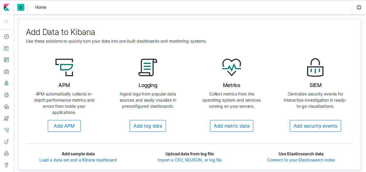
Figure 7-1. Kibana’s landing dashboard page

Hit the local instance of Nginx to get some activity in the logs and start the data processing. For this example, the Apache Benchmarking Tool (ab) is used, but you can try it with your browser or directly with curl:

$ ab -c 8 -n 50 http://localhost/
This is ApacheBench, Version 2.3 <$Revision: 1430300 $>
Copyright 1996 Adam Twiss, Zeus Technology Ltd, http://www.zeustech.net/
Licensed to The Apache Software Foundation, http://www.apache.org/

Benchmarking localhost (be patient).....done

Without doing anything specific to configure Kibana further, open the default URL and port where it is running: http://localhost:5601. The default view offers lots of options to add. In the discover section, you will see all the structured information from the requests. This is an example JSON fragment that Logstash processed and is available in Kibana (which is sourcing the data from Elasticsearch):

...
    "input": {
      "type": "log"
    },
    "auth": "-",
    "ident": "-",
    "request": "/",
    "response": "200",
    "@timestamp": "2019-08-08T21:03:46.513Z",
    "verb": "GET",
    "@version": "1",
    "referrer": ""-"",
    "httpversion": "1.1",
    "message": "::1 - - [08/Aug/2019:21:03:45 +0000] "GET / HTTP/1.1" 200",
    "clientip": "::1",
    "geoip": {},
    "ecs": {
      "version": "1.0.1"
    },
    "host": {
      "os": {
        "codename": "Core",
        "name": "CentOS Linux",
        "version": "7 (Core)",
        "platform": "centos",
        "kernel": "3.10.0-957.1.3.el7.x86_64",
        "family": "redhat"
      },
      "id": "0a75ccb95b4644df88f159c41fdc7cfa",
      "hostname": "node2",
      "name": "node2",
      "architecture": "x86_64",
      "containerized": false
    },
    "bytes": "3700"
  },
  "fields": {
    "@timestamp": [
      "2019-08-08T21:03:46.513Z"
    ]
  }
...

Critical keys like verb, timestamp, request, and response have been parsed and captured by Logstash. There is lots of work to do with this initial setup to convert it into something more useful and practical. The captured metadata can help render traffic (including geolocation), and Kibana can even set threshold alerts for data, for when specific metrics go above or below a determined value.

In the dashboard, this structured data is available to be picked apart and used to create meaningful graphs and representations, as shown in Figure 7-2.

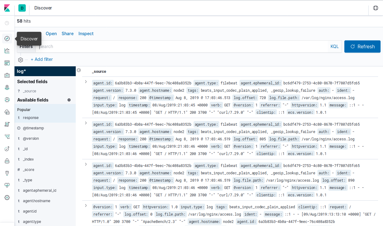
Figure 7-2. Structured data in Kibana

As we’ve seen, the ELK stack can get you started capturing and parsing through logs with minimal configuration and almost no effort. The examples are trivial, but should already demonstrate the immense capabilities of its components. More often than we would like to admit, we’ve been faced with infrastructure with a cron entry that is tailing logs and grepping for some pattern to send an email or submit an alert to Nagios. Using capable software components and understanding how much they can do for you, even in their simplest forms, is essential to better infrastructure, and in this case, better visibility of what that infrastructure is doing.