Measuring Performance

If we had to work in an isolated environment with a server that doesn’t have access to the internet or that we don’t control and therefore can’t install packages, we would have to say that the dd tool (which should be readily available on all major Linux distributions) would help provide some answers. If at all possible, pair it with iostat to isolate the command that hammers the device versus the one that gets the report.

As a seasoned performance engineer once said, it depends on what is measured and how. For example dd is single threaded and has limitations, such as being unable to do multiple random reads and writes; it also measures throughput and not input/output operations per second (IOPS). What are you measuring? Throughput or IOPS?

This simple one-liner will run dd to get some numbers of a brand-new device (/dev/sdc in this case):

$ dd if=/dev/zero of=/dev/sdc count=10 bs=100M
10+0 records in
10+0 records out
1048576000 bytes (1.0 GB, 1000 MiB) copied, 1.01127 s, 1.0 GB/s

It writes 10 records of 100 megabytes at a rate of 1 GB/s. This is throughput. An easy way to get IOPS with dd is to use iostat. In this example, iostat runs only on the device getting hammered with dd, with the -d flag only to give the device information, and with an interval of one second:

$ iostat -d /dev/sdc 1

Device             tps    kB_read/s    kB_wrtn/s    kB_read    kB_wrtn
sdc            6813.00         0.00   1498640.00          0    1498640

Device             tps    kB_read/s    kB_wrtn/s    kB_read    kB_wrtn
sdc            6711.00         0.00   1476420.00          0    1476420

The iostat output will repeat itself for every second until a Ctrl-C is issued to cancel the operation. The second column in the output is tps, which stands for transactions per second and is the same as IOPS. A nicer way to visualize the output, which avoids the clutter that a repeating command produces, is to clear the terminal on each run:

$ while true; do clear && iostat -d /dev/sdc && sleep 1; done

$ fio --name=sdc-performance --filename=/dev/sdc --ioengine=libaio 
  --iodepth=1 --rw=randrw --bs=32k --direct=0 --size=64m
sdc-performance: (g=0): rw=randwrite, bs=(R) 32.0KiB-32.0KiB,
(W) 32.0KiB-32.0KiB, (T) 32.0KiB-32.0KiB, ioengine=libaio, iodepth=1
fio-3.1
Starting 1 process

sdc-performance: (groupid=0, jobs=1): err= 0: pid=2879:
   read: IOPS=1753, BW=54.8MiB/s (57.4MB/s)(31.1MiB/567msec)
...
   iops        : min= 1718, max= 1718, avg=1718.00, stdev= 0.00, samples=1
  write: IOPS=1858, BW=58.1MiB/s (60.9MB/s)(32.9MiB/567msec)
...
   iops        : min= 1824, max= 1824, avg=1824.00, stdev= 0.00, samples=1

Partitions

We tend to default to fdisk with its interactive session to create partitions, but in some cases, fdisk doesn’t work well, such as with large partitions (two terabytes or larger). In those cases, your fallback should be to use parted.

A quick interactive session shows how to create a primary partition with fdisk, with the default start value and four gibibytes of size. At the end the w key is sent to write the changes:

$ sudo fdisk /dev/sds

Command (m for help): n
Partition type:
   p   primary (0 primary, 0 extended, 4 free)
   e   extended
Select (default p): p
Partition number (1-4, default 1):
First sector (2048-22527999, default 2048):
Using default value 2048
Last sector, +sectors or +size{K,M,G} (2048-22527999, default 22527999): +4G
Partition 1 of type Linux and of size 4 GiB is set

Command (m for help): w
The partition table has been altered!

Calling ioctl() to re-read partition table.
Syncing disks.

parted accomplishes the same, but with a different interface:

$ sudo parted /dev/sdaa
GNU Parted 3.1
Using /dev/sdaa
Welcome to GNU Parted! Type 'help' to view a list of commands.
(parted) mklabel
New disk label type? gpt
(parted) mkpart
Partition name?  []?
File system type?  [ext2]?
Start? 0
End? 40%

In the end, you quit with the q key. For programmatic creation of partitions on the command line without any interactive prompts, you accomplish the same result with a couple of commands:

$ parted --script /dev/sdaa mklabel gpt
$ parted --script /dev/sdaa mkpart primary 1 40%
$ parted --script /dev/sdaa print
Disk /dev/sdaa: 11.5GB
Sector size (logical/physical): 512B/512B
Partition Table: gpt
Disk Flags:

Number  Start   End     Size    File system  Name     Flags
 1      1049kB  4614MB  4613MB

Retrieving Specific Device Information

Sometimes when specific information for a device is needed, either lsblk or blkid are well suited. fdisk doesn’t like to work without superuser permissions. Here fdisk lists the information about the /dev/sda device:

$ fdisk -l /dev/sda
fdisk: cannot open /dev/sda: Permission denied

$ sudo fdisk -l /dev/sda

Disk /dev/sda: 42.9 GB, 42949672960 bytes, 83886080 sectors
Units = sectors of 1 * 512 = 512 bytes
Sector size (logical/physical): 512 bytes / 512 bytes
I/O size (minimum/optimal): 512 bytes / 512 bytes
Disk label type: dos
Disk identifier: 0x0009d9ce

   Device Boot      Start         End      Blocks   Id  System
/dev/sda1   *        2048    83886079    41942016   83  Linux

blkid is a bit similar in that it wants superuser permissions as well:

$ blkid /dev/sda

$ sudo blkid /dev/sda
/dev/sda: PTTYPE="dos"

lsblk allows to get information without higher permissions, and provides the same informational output regardless:

$ lsblk /dev/sda
NAME   MAJ:MIN RM SIZE RO TYPE MOUNTPOINT
sda      8:0    0  40G  0 disk
└─sda1   8:1    0  40G  0 part /
$ sudo lsblk /dev/sda
NAME   MAJ:MIN RM SIZE RO TYPE MOUNTPOINT
sda      8:0    0  40G  0 disk
└─sda1   8:1    0  40G  0 part /

This command, which uses the -p flag for low-level device probing, is very thorough and should give you good enough information for a device:

$ blkid -p /dev/sda1
UUID="8e4622c4-1066-4ea8-ab6c-9a19f626755c" TYPE="xfs" USAGE="filesystem"
PART_ENTRY_SCHEME="dos" PART_ENTRY_TYPE="0x83" PART_ENTRY_FLAGS="0x80"
PART_ENTRY_NUMBER="1" PART_ENTRY_OFFSET="2048" PART_ENTRY_SIZE="83884032"

lsblk has some default properties to look for:

$ lsblk -P /dev/nvme0n1p1
NAME="nvme0n1p1" MAJ:MIN="259:1" RM="0" SIZE="512M" RO="0" TYPE="part"

But it also allows you to set specific flags to request a particular property:

lsblk -P -o SIZE /dev/nvme0n1p1
SIZE="512M"

To access a property in this way makes it easy to script and even consume from the Python side of things.

SSH Tunneling

Have you ever tried to reach an HTTP service that runs on a remote server that is not accessible except via SSH? This situation occurs when the HTTP service is enabled but not needed publicly. The last time we saw this happen was when a production instance of RabbitMQ had the management plug-in enabled, which starts an HTTP service on port 15672. The service isn’t exposed and with good reason; there is no need to have it publicly available since it is rarely used, and besides, one can use SSH’s tunneling capabilities.

This works by creating an SSH connection with the remote server and then forwarding the remote port (15672, in my case) to a local port on the originating machine. The remote machine has a custom SSH port, which complicates the command slightly. This is is how it looks:

$ ssh -L 9998:localhost:15672 -p 2223 [email protected] -N

There are three flags, three numbers, and two addresses. Let’s dissect the command to make what is going on here much clearer. The -L flag is the one that signals that we want forwarding enabled and a local port (9998) to bind to a remote port (RabbitMQ’s default of 15672). Next, the -p flag indicates that the custom SSH port of the remote server is 2223, and then the username and address are specified. Lastly, the -N means that it shouldn’t get us to a remote shell and do the forwarding.

When executed correctly, the command will appear to hang, but it allows you to go into http://localhost:9998/ and see the login page for the remote RabbitMQ instance. A useful flag to know when tunneling is -f: it will send the process into the background, which is helpful if this connection isn’t temporary, leaving the terminal ready and clean to do more work.

Benchmarking HTTP with Apache Benchmark (ab)

We really love to hammer servers we work with to ensure they handle load correctly, especially before they get promoted to production. Sometimes we even try to trigger some odd race condition that may happen under heavy load. The Apache Benchmark tool (ab in the command line) is one of those tiny tools that can get you going quickly with just a few flags.

This command will create 100 requests at a time, for a total of 10,000 requests, to a local instance where Nginx is running:

$ ab -c 100 -n 10000 http://localhost/

That is pretty brutal to handle in a system, but this is a local server, and the requests are just an HTTP GET. The detailed output from ab is very comprehensive and looks like this (trimmed for brevity):

Benchmarking localhost (be patient)
...
Completed 10000 requests
Finished 10000 requests

Server Software:        nginx/1.15.9
Server Hostname:        localhost
Server Port:            80

Document Path:          /
Document Length:        612 bytes

Concurrency Level:      100
Time taken for tests:   0.624 seconds
Complete requests:      10000
Failed requests:        0
Total transferred:      8540000 bytes
HTML transferred:       6120000 bytes
Requests per second:    16015.37 [#/sec] (mean)
Time per request:       6.244 [ms] (mean)
Time per request:       0.062 [ms] (mean, across all concurrent requests)
Transfer rate:          13356.57 [Kbytes/sec] received

Connection Times (ms)
              min  mean[+/-sd] median   max
Connect:        0    3   0.6      3       5
Processing:     0    4   0.8      3       8
Waiting:        0    3   0.8      3       6
Total:          0    6   1.0      6       9

This type of information and how it is presented is tremendous. At a glance, you can quickly tell if a production server drops connections (in the Failed requests field) and what the averages are. A GET request is used, but ab allows you to use other HTTP verbs, such as POST, and even do a HEAD request. You need to exercise caution with this type of tool because it can easily overload a server. Below are more realistic numbers from an HTTP service in production (trimmed for brevity):

...
Benchmarking prod1.ceph.internal (be patient)

Server Software:        nginx
Server Hostname:        prod1.ceph.internal
Server Port:            443
SSL/TLS Protocol:       TLSv1.2,ECDHE-RSA-AES256-GCM-SHA384,2048,256
Server Temp Key:        ECDH P-256 256 bits
TLS Server Name:        prod1.ceph.internal

Complete requests:      200
Failed requests:        0
Total transferred:      212600 bytes
HTML transferred:       175000 bytes
Requests per second:    83.94 [#/sec] (mean)
Time per request:       1191.324 [ms] (mean)
Time per request:       11.913 [ms] (mean, across all concurrent requests)
Transfer rate:          87.14 [Kbytes/sec] received
....

Now the numbers look different, it hits a service with SSL enabled, and ab lists what the protocols are. At 83 requests per second, we think it could do better, but this is an API server that produces JSON, and it typically doesn’t get much load at once, as was just generated.

Load Testing with molotov

The Molotov project is an interesting project geared towards load testing. Some of its features are similar to those of Apache Benchmark, but being a Python project, it provides a way to write scenarios with Python and the asyncio module.

This is how the simplest example for molotov looks:

import molotov

@molotov.scenario(100)
async def scenario_one(session):
    async with session.get("http://localhost:5000") as resp:
        assert resp.status == 200

Save the file as load_test.py, create a small Flask application that handles both POST and GET requests at its main URL, and save it as small.py:

from flask import Flask, redirect, request

app = Flask('basic app')

@app.route('/', methods=['GET', 'POST'])
def index():
    if request.method == 'POST':
        redirect('https://www.google.com/search?q=%s' % request.args['q'])
    else:
        return '<h1>GET request from Flask!</h1>'

Start the Flask application with FLASK_APP=small.py flask run, and then run molotov with the load_test.py file created previously:

$ molotov -v -r 100 load_test.py
**** Molotov v1.6. Happy breaking! ****
Preparing 1 worker...
OK
SUCCESSES: 100 | FAILURES: 0 WORKERS: 0
*** Bye ***

One hundred requests on a single worker ran against the local Flask instance. The tool really shines when the load testing is extended to do more per request. It has concepts similar to unit testing, such as setup, teardown, and even code, that can react to certain events. Since the small Flask application can handle a POST that redirects to a Google search, add another scenario to the load_test.py_ file. This time change the weight so that 100% of the requests do a POST:

@molotov.scenario(100)
async def scenario_post(session):
    resp = await session.post("http://localhost:5000", params={'q': 'devops'})
    redirect_status = resp.history[0].status
    error = "unexpected redirect status: %s" % redirect_status
    assert redirect_status == 301, error

Run this new scenario for a single request to show the following:

$ molotov -v -r 1 --processes 1 load_test.py
**** Molotov v1.6. Happy breaking! ****
Preparing 1 worker...
OK
AssertionError('unexpected redirect status: 302',)
  File ".venv/lib/python3.6/site-packages/molotov/worker.py", line 206, in step
    **scenario['kw'])
  File "load_test.py", line 12, in scenario_two
    assert redirect_status == 301, error
SUCCESSES: 0 | FAILURES: 1
*** Bye ***

A single request (with -r 1) was enough to make this fail. The assertion needs to be updated to check for a 302 instead of a 301. Once that status is updated, change the weight of the POST scenario to 80 so that other requests (with a GET) are sent to the Flask application. This is how the file looks in the end:

import molotov

@molotov.scenario()
async def scenario_one(session):
    async with session.get("http://localhost:5000/") as resp:
        assert resp.status == 200

@molotov.scenario(80)
async def scenario_two(session):
    resp = await session.post("http://localhost:5000", params={'q': 'devops'})
    redirect_status = resp.history[0].status
    error = "unexpected redirect status: %s" % redirect_status
    assert redirect_status == 301, error

Run load_test.py for 10 requests to distribute the requests, two for a GET and the rest with a POST:

127.0.0.1 - - [04/Sep/2019 12:10:54] "POST /?q=devops HTTP/1.1" 302 -
127.0.0.1 - - [04/Sep/2019 12:10:56] "POST /?q=devops HTTP/1.1" 302 -
127.0.0.1 - - [04/Sep/2019 12:10:57] "POST /?q=devops HTTP/1.1" 302 -
127.0.0.1 - - [04/Sep/2019 12:10:58] "GET / HTTP/1.1" 200 -
127.0.0.1 - - [04/Sep/2019 12:10:58] "POST /?q=devops HTTP/1.1" 302 -
127.0.0.1 - - [04/Sep/2019 12:10:59] "POST /?q=devops HTTP/1.1" 302 -
127.0.0.1 - - [04/Sep/2019 12:11:00] "POST /?q=devops HTTP/1.1" 302 -
127.0.0.1 - - [04/Sep/2019 12:11:01] "GET / HTTP/1.1" 200 -
127.0.0.1 - - [04/Sep/2019 12:11:01] "POST /?q=devops HTTP/1.1" 302 -
127.0.0.1 - - [04/Sep/2019 12:11:02] "POST /?q=devops HTTP/1.1" 302 -

As you can see, molotov is easily extensible with pure Python and can be modified to suit other, more complex, needs. These examples scratch the surface of what the tool can do.

Viewing Processes with htop

The htop tool is just like top (an interactive process viewer) but is fully cross-platform (works on OS X, FreeBSD, OpenBSD, and Linux), offers support for better visualizations (see Figure 4-1), and is a pleasure to use. Visit https://hisham.hm/htop for a screenshot of htop running on a server. One of the main caveats of htop is that all the shortcuts you may know about top are not compatible, so you will have to rewire your brain to understand and use them for htop.

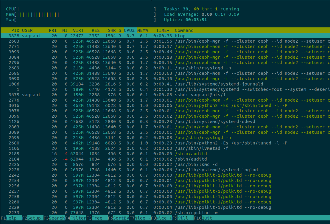
Figure 4-1. htop running on a server

Right away, the look and feel of the information displayed in Figure 4-1 is different. The CPU, Memory, and Swap are nicely shown at the top left, and they move as the system changes. The arrow keys scroll up or down and even left to right, providing a view of the whole command of the process.

Want to kill a process? Move to it with the arrow keys, or hit / to incrementally search (and filter) the process, and then press k. A new menu will show all the signals that can be sent to the process—for example, SIGTERM instead of SIGKILL. It is possible to “tag” more than one process to kill. Press the space bar to tag the selected process, highlighting it with a different color. Made a mistake and want to un-tag? Press the space bar again. This all feels very intuitive.

One problem with htop is that it has lots of actions mapped to F keys, and you may not have any. For example, F1 is for help. The alternative is to use the equivalent mappings when possible. To access the help menu, use the h key; to access the setup, use Shift s instead of F2.

The t (again, how intuitive!) enables (toggles) the process list as a tree. Probably the most used functionality is sorting. Press > and a menu appears to select what type of sorting you want: PID, user, memory, priority, and CPU percentage are just a few. There are also shortcuts to sort directly (skips the menu selection) by memory (Shift i), CPU (Shift p), and Time (Shift t).

Finally, two incredible features: you can run strace or lsof directly in the selected process as long as these are installed and available to the user. If the processes require superuser permissions, htop will report that, and it will require sudo to run as a privileged user. To run strace on a selected process, use the s key; for lsof, use the l key.

If either strace or lsof is used, the search and filter options are available with the / character. What an incredibly useful tool! Hopefully, one day other non-F key mappings will be possible, even though most work can be done with the alternative mappings.

Customizing the Python Shell

You can customize the Python shell with helpers and import useful modules in a Python file that then has to be exported as an environment variable. I keep my configuration files in a repository called dotfiles, so in my shell configuration file ($HOME/.zshrc for me) I define the following export:

export PYTHONSTARTUP=$HOME/dotfiles/pythonstartup.py

To try this out, create a new Python file called pythonstartup.py (although it can be named anything) that looks like this:

import types
import uuid

helpers = types.ModuleType('helpers')
helpers.uuid4 = uuid.uuid4()

Now open up a new Python shell and specify the newly created pythonstartup.py:

$ PYTHONSTARTUP=pythonstartup.py python
Python 3.7.3 (default, Apr  3 2019, 06:39:12)
[GCC 8.3.0] on linux
Type "help", "copyright", "credits" or "license" for more information.
>>> helpers
<module 'helpers'>
>>> helpers.uuid4()
UUID('966d7dbe-7835-4ac7-bbbf-06bf33db5302')

The helpers object is immediately available. Since we added the uuid4 property, we can access it as helpers.uuid4(). As you may be able to tell, all the imports and definitions are going to be available in the Python shell. This is a convenient way to extend behavior that can be useful with the default shell.

Recursive Globbing

Recursive globbing is enabled in ZSH by default, but Bash (versions 4 and higher) requires shopt to set it. Recursive globbing is a cool setting that allows you to traverse a path with the following syntax:

$ ls **/*.py

That snippet would go through each file and directory recursively and list every single file that ends in .py. This is how to enable it in Bash 4:

$ shopt -s globstar

Searching and Replacing with Confirmation Prompts

Vim has a nice feature in its search and replace engine that prompts for confirmation to perform the replacement or skip it. This is particularly useful when you can’t nail the exact regular expression that matches what you need but want to ignore some other close matches. We know regular expressions, but we’ve tried to avoid being an expert at them because it would be very tempting to use them for everything. Most of the time, you will want to perform a simple search and replace and not bang your head against the wall to come up with the perfect regex.

The c flag needs to be appended at the end of the command to enable the confirmation prompt in Vim:

:%s/original term/replacement term/gc

The above translates to: search for original term in the whole file and replace it with replacement term, but at each instance, prompt so that one can decide to change it or skip it. If a match is found, Vim will display a message like this one:

replace with replacement term (y/n/a/q/l/^E/^Y)?

The whole confirmation workflow might seem silly but allows you to relax the constraints on the regular expression, or even not use one at all for a simpler match and replace. A quick example of this is a recent API change in a production tool that changed an object’s attribute for a callable. The code returned True or False to inform if superuser permissions were required or not. The actual replacement in a single file would look like this:

:%s/needs_root/needs_root()/gc

The added difficulty here is that needs_root was also splattered in comments and doc strings, so it wasn’t easy to come up with a regular expression that would allow skipping the replacement when inside a comment block or in part of a doc string. With the c flag, you can just hit Y or N and move on. No regular expression needed at all!

With recursive globbing enabled (shopt -s globstar in Bash 4), this powerful one-liner will go through all the matching files, perform the search, and replace the item according to the prompts if the pattern is found inside the files:

vim -c "bufdo! set eventignore-=Syntax | %s/needs_root/needs_root()/gce" **/*.py

There is a lot to unpack here, but the above example will traverse recursively to find all the files ending in .py, load them into Vim, and perform the search and replace with confirmation only if there is a match. If there isn’t a match, it skips the file. The set eventignore-=Syntax is used because otherwise Vim will not load the syntax files when executing it this way; we like syntax highlighting and expect it to work when this type of replacement is used. The next part after the | character is the replacement with the confirmation flag and the e flag, which helps ignore any errors that would prevent a smooth workflow from being interrupted with errors.

Make the complicated one-liner easier to remember with a function that takes two parameters (search and replace terms) and the path:

vsed() {
  search=$1
  replace=$2
  shift
  shift
  vim -c "bufdo! set eventignore-=Syntax| %s/$search/$replace/gce" $*
}

Name it vsed, as a mix of Vim and the sed tool, so that it is easier to remember. In the terminal, it looks straightforward and allows you to make changes to multiple files easily and with confidence, since you can accept or deny each replacement:

$ vsed needs_root needs_root() **/*.py

Removing Temporary Python Files

Python’s pyc, and more recently its pycache directories, can sometimes get in the way. This simple one-liner aliased to pyclean uses the find command to remove pyc, then goes on to find pycache directories and recursively deletes them with the tool’s built-in delete flag:

alias pyclean='find . 
    ( -type f -name "*.py[co]" -o -type d -name "__pycache__" ) -delete &&
    echo "Removed pycs and __pycache__"'

Listing and Filtering Processes

Process listing to view what runs in a machine and then filtering to check on a specific application is one of the things that you’ll do several times a day at the very least. It is not at all surprising that everyone has a variation on either the flags or the order of the flags for the ps tool (we usually use aux). It is something you end up doing so many times a day that the order and the flags get ingrained in your brain and it is hard to do it any other way.

As a good starting point to list the processes and some information, such as process IDs, try this:

$ ps auxw

This command lists all processes with the BSD-style flags (flags that aren’t prefixed with a dash -) regardless or whether they have a terminal (tty) or not, and includes the user that owns the process. Finally, it gives more space to the output (w flag).

Most of the times, you are filtering with grep to get information about a specific process. For example, if you want to check if Nginx is running, you pipe the output into grep and pass nginx as an argument:

$ ps auxw | grep nginx
root     29640  1536 ?        Ss   10:11   0:00 nginx: master process
www-data 29648  5440 ?        S    10:11   0:00 nginx: worker process
alfredo  30024   924 pts/14   S+   10:12   0:00 grep nginx

That is great, but it is annoying to have the grep command included. This is particularly maddening when there are no results except for the grep:

$ ps auxw | grep apache
alfredo  31351  0.0  0.0   8856   912 pts/13   S+   10:15   0:00 grep apache

No apache process is found, but the visuals may mislead you to think it is, and double-checking that this is indeed just grep being included because of the argument can get tiring pretty quickly. A way to solve this is to add another pipe to grep to filter itself from the output:

$ ps auxw | grep apache | grep -v grep

To have to always remember to add that extra grep can be equally annoying, so an alias comes to the rescue:

alias pg='ps aux | grep -v grep | grep $1'

The new alias will filter the first grep line out and leave only the interesting output (if any):

$ pg vim
alfredo  31585  77836 20624 pts/3    S+   18:39   0:00 vim /home/alfredo/.zshrc

Unix Timestamp

To get the widely used Unix timestamp in Python is very easy:

In [1]: import time

In [2]: int(time.time())
Out[2]: 1566168361

But in the shell, it can be a bit more involved. This alias works in OS X, which has the BSD-flavored version of the date tool:

alias timestamp='date -j -f "%a %b %d %T %Z %Y" "`date`" "+%s"'

OS X can be awkward with its tooling, and it may be confusing to never remember why a given utility (like date in this case) behaves completely differently. In the Linux version of date, a far simpler approach works the same way:

alias timestamp='date "+%s"'

Random Password Generator

The amount of accounts and passwords that you need on a week-to-week basis is only going to keep increasing, even for throwaway accounts that you can use Python for to generate robust passwords. Create a useful, randomized password generator that sends the contents to the clipboard to easily paste it:

In [1]: import os

In [2]: import base64

In [3]: print(base64.b64encode(os.urandom(64)).decode('utf-8'))
gHHlGXnqnbsALbAZrGaw+LmvipTeFi3tA/9uBltNf9g2S9qTQ8hTpBYrXStp+i/o5TseeVo6wcX2A==

Porting that to a shell function that can take an arbitrary length (useful when a site restricts length to a certain number) looks like this:

mpass() {
    if [ $1 ]; then
        length=$1
    else
        length=12
    fi
    _hash=`python3 -c "
import os,base64
exec('print(base64.b64encode(os.urandom(64))[:${length}].decode('utf-8'))')
    "`
    echo $_hash | xclip -selection clipboard
    echo "new password copied to the system clipboard"
}

Now the mpass function defaults to generate 12-character passwords by slicing the output, and then sends the contents of the generated string to xclip so that it gets copied to the clipboard for easy pasting.

Does My Module Exist?

Find out if a module exists, and if it does, get the path to that module. This is useful when reused for other functions that can take that output for processing:

try() {
    python -c "
exec('''
try:
    import ${1} as _
    print(_.__file__)
except Exception as e:
    print(e)
''')"
}

Debuggers

A few programmers out there swear by the print() statement as the best strategy to debug running code. In some cases, that might work fine, but most of the time we use the Python debugger (with the pdb module) or ipdb, which uses IPython as a backend. By creating a break point, you can poke around at variables and go up and down the stack. These single-line statements are important enough that you should memorize them:

Set a break point and drop to the Python debugger (pdb):

import pdb;pdb.set_trace()

Set a break point and drop to a Python debugger based on IPython (ipdb):

import ipdb;ipdb.set_trace()

Although not technically a debugger (you can’t move forward or backward in the stack), this one-liner allows you to start an IPython session when the execution gets to it:

import IPython; IPython.embed()

How Fast Is this Snippet?

Python has a module to run a piece of code several times over and get some performance metrics from it. Lots of users like to ask if there are efficient ways to handle a loop or update a dictionary, and there are lots of knowledgeable people that love the timeit module to prove performance.

As you have probably seen, we are fans of IPython, and its interactive shell comes with a “magic” special function for the timeit module. “Magic” functions are prefixed with the % character and perform a distinct operation within the shell. An all-time favorite regarding performance is whether list comprehension is faster than just appending to a list. The two examples below use the timeit module to find out:

In [1]: def f(x):
   ...:     return x*x
   ...:

In [2]: %timeit for x in range(100): f(x)
100000 loops, best of 3: 20.3 us per loop

In the standard Python shell (or interpreter), you import the module and access it directly. The invocation looks a bit different in this case:

>>> array = []
>>> def appending():
...     for i in range(100):
...         array.append(i)
...
>>> timeit.repeat("appending()", "from __main__ import appending")
[5.298534262983594, 5.32031941099558, 5.359099322988186]
>>> timeit.repeat("[i for i in range(100)]")
[2.2052824340062216, 2.1648171059787273, 2.1733458579983562]

The output is a bit odd, but that’s because it’s meant to be processed by another module or library, and is not meant for human readability. The averages favor the list comprehension. This is how it looks in IPython:

In [1]: def appending():
   ...:     array = []
   ...:     for i in range(100):
   ...:         array.append(i)
   ...:

In [2]: %timeit appending()
5.39 µs ± 95.1 ns per loop (mean ± std. dev. of 7 runs, 100000 loops each)

In [3]: %timeit [i for i in range(100)]
2.1 µs ± 15.2 ns per loop (mean ± std. dev. of 7 runs, 100000 loops each)

Because IPython exposes timeit as a special command (notice the prefix with %), the output is human readable and more helpful to view, and it doesn’t require the weird import, as in the standard Python shell.