
10
Monte Carlo Simulations in Finance
Monte Carlo simulations are a class of computational algorithms that use repeated random sampling to solve any problems that have a probabilistic interpretation. In finance, one of the reasons they gained popularity is that they can be used to accurately estimate integrals. The main idea of Monte Carlo simulations is to produce a multitude of sample paths (possible scenarios/outcomes), often over a given period of time. The horizon is then split into a specified number of time steps and the process of doing so is called discretization. Its goal is to approximate the continuous time in which the pricing of financial instruments happens.
The results from all of these simulated sample paths can be used to calculate metrics such as the percentage of times an event occurred, the average value of an instrument at the last step, and so on. Historically, the main problem with the Monte Carlo approach was that it required heavy computational power to calculate all of the considered scenarios. Nowadays, this is becoming less of a problem as we can run fairly advanced simulations on a desktop computer or a laptop, and if we run out of computing power, we can use cloud computing and its more powerful processors.
By the end of this chapter, we will have seen how we can use Monte Carlo methods in various scenarios and tasks. In some of them, we will create the simulations from scratch, while in others, we will use modern Python libraries to make the process even easier. Due to the method’s flexibility, Monte Carlo is one of the most important techniques in computational finance. It can be adapted to various problems, such as pricing derivatives with no closed-form solution (American/exotic options), valuation of bonds (for example, a zero-coupon bond), estimating the uncertainty of a portfolio (for example, by calculating Value-at-Risk and Expected Shortfall), and carrying out stress tests in risk management. We will show you how to solve some of these problems in this chapter.
In this chapter, we cover the following recipes:
- Simulating stock price dynamics using a geometric Brownian motion
- Pricing European options using simulations
- Pricing American options with Least Squares Monte Carlo
- Pricing American options using QuantLib
- Pricing barrier options
- Estimating Value-at-Risk using Monte Carlo
Simulating stock price dynamics using a geometric Brownian motion
Simulating stock prices plays a crucial role in the valuation of many derivatives, most notably options. Due to the randomness in the price movement, these simulations rely on stochastic differential equations (SDEs). A stochastic process is said to follow a geometric Brownian motion (GBM) when it satisfies the following SDE:
![]()
Here, we have the following:
- St—Stock price
 —The drift coefficient, that is, the average return over a given period or the instantaneous expected return
 —The diffusion coefficient, that is, how much volatility is in the drift
- Wt —The Brownian motion
- d—This symbolizes the change in the variable over the considered time increment, while dt is the change in time
We will not investigate the properties of the Brownian motion in too much depth, as it is outside the scope of this book. Suffice to say, Brownian increments are calculated as a product of a Standard Normal random variable ![]() and the square root of the time increment.
and the square root of the time increment.
Another way to say this is that the Brownian increment comes from ![]() , where t is the time increment. We obtain the Brownian path by taking the cumulative sum of the Brownian increments.
, where t is the time increment. We obtain the Brownian path by taking the cumulative sum of the Brownian increments.
The SDE mentioned above is one of the few that has a closed-form solution:
![]()
Where S0 = S(0) is the initial value of the process, which in this case is the initial price of a stock. The preceding equation presents the relationship between the stock price at time t and the initial stock price.
For simulations, we can use the following recursive formula:
![]()
Where Zi is a Standard Normal random variable and i = 0, 1, …, T-1 is the time index. This specification is possible because the increments of W are independent and normally distributed. Please refer to Euler’s discretization for a better understanding of the formula’s origin.
A GBM is a process that does not account for mean-reversion and time-dependent volatility. That is why it is often used for stocks and not for bond prices, which tend to display long-term reversion to the face value.
In this recipe, we use Monte Carlo methods and a GBM to simulate IBM’s stock prices one month ahead—using data from 2021, we will simulate the possible paths over January 2022.
How to do it...
Execute the following steps to simulate IBM’s stock prices one month ahead:
- Import the libraries:
import numpy as np import pandas as pd import yfinance as yf - Download IBM’s stock prices from Yahoo Finance:
df = yf.download("IBM", start="2021-01-01", end="2022-01-31", adjusted=True) - Calculate and plot the daily returns:
returns = df["Adj Close"].pct_change().dropna()
returns.plot(title="IBM's returns")
Running the snippet produces the following plot:
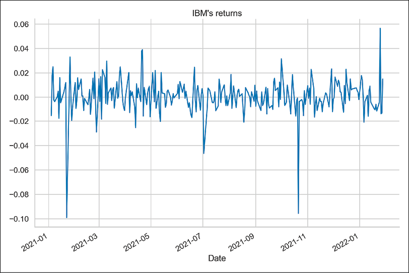
Figure 10.1: IBM’s simple returns
- Split the data into training and test sets:
train = returns["2021"] test = returns["2022"] - Specify the parameters of the simulation:
T = len(test) N = len(test) S_0 = df.loc[train.index[-1], "Adj Close"] N_SIM = 100 mu = train.mean() sigma = train.std() - Define the function used for the simulations:
def simulate_gbm(s_0, mu, sigma, n_sims, T, N, random_seed=42): np.random.seed(random_seed) dt = T/N dW = np.random.normal(scale=np.sqrt(dt), size=(n_sims, N)) W = np.cumsum(dW, axis=1) time_step = np.linspace(dt, T, N) time_steps = np.broadcast_to(time_step, (n_sims, N)) S_t = ( s_0 * np.exp((mu - 0.5 * sigma**2) * time_steps + sigma * W) ) S_t = np.insert(S_t, 0, s_0, axis=1) return S_t - Run the simulations and store the results in a DataFrame:
gbm_simulations = simulate_gbm(S_0, mu, sigma, N_SIM, T, N) sim_df = pd.DataFrame(np.transpose(gbm_simulations), index=train.index[-1:].union(test.index)) - Create a DataFrame with the average value for each time step and the corresponding actual stock price:
res_df = sim_df.mean(axis=1).to_frame() res_df = res_df.join(df["Adj Close"]) res_df.columns = ["simulation_average", "adj_close_price"] - Plot the results of the simulation:
ax = sim_df.plot(
    alpha=0.3, legend=False, title="Simulation's results"
)
res_df.plot(ax=ax, color = ["red", "blue"])
In Figure 10.2, we observe that the predicted stock prices (the averages of the simulations for each time step) exhibit a slightly positive trend. That could be attributed to the positive drift term
 = 0.07%. However, we should take that conclusion with a pinch of salt given the very small number of simulations.

Figure 10.2: The simulated paths together with their average
Bear in mind that such a visualization is only feasible for a reasonable number of sample paths. In real-life cases, we want to use significantly more sample paths than 100. The general approach to Monte Carlo simulations is that having more sample paths leads to more accurate/reliable results.
How it works...
In Steps 2 and 3, we downloaded IBM’s stock prices and calculated simple returns. In the next step, we divided the data into the training and test sets. While there is no explicit training of any model here, we used the training set to calculate the average and standard deviation of the returns. We then used those values as the drift (mu) and diffusion (sigma) coefficients for our simulations. Additionally, in Step 5, we defined the following parameters:
T: Forecasting horizon; in this case, the number of days in the test set.N: Number of time increments in the forecasting horizon. For our simulation, we keepN=T.S_0: Initial price. For this simulation, we use the last observation from the training set.N_SIM: Number of simulated paths.
Monte Carlo simulations use a process called discretization. The idea is to approximate the continuous pricing of financial assets by splitting the considered time horizon into a large number of discrete intervals. That is why, except for considering the forecasting horizon, we also need to indicate the number of time increments to fit into the horizon.
In Step 6, we defined the function for running the simulations. It is good practice to define a function/class for such a problem, as it will also come in handy in the following recipes. The function executes the following steps:
- Defines the time increment (
dt) and the Brownian increments (dW). In the matrix of Brownian increments (size:N_SIM×N), each row describes one sample path. - Calculates the Brownian paths (
W) by running a cumulative sum (np.cumsum) over the rows. - Creates a matrix containing the time steps (
time_steps). To do so, we created an array of evenly spaced values within an interval (the horizon of the simulation). For that, we used thenp.linspacefunction. Afterward, we broadcasted the array to the intended shape usingnp.broadcast_to. - Calculates the stock price at each point in time using the closed-form formula.
- Inserts the initial value into the first position of each row.
There was no explicit need to broadcast the vector containing time steps. It would have been done automatically to match the required dimensions (the dimension of W). By doing it manually, we get more control over what we are doing, which makes the code easier to debug. We should also be aware that in languages such as R, there is no automatic broadcasting.
In the function’s definition, we can recognize the drift as (mu - 0.5 * sigma ** 2) * time_steps and the diffusion as sigma * W. Additionally, while defining this function, we followed the vectorized approach. By doing so, we avoided writing any for loops, which would be inefficient in the case of large simulations.
For reproducible results, use np.random.seed before simulating the paths.
In Step 7, we ran the simulations and stored the outcome (sample paths) in a DataFrame. While doing so, we transposed the data so that we had one path per column, which simplifies using the plot method of the pandas DataFrame. To have the appropriate index, we used the union method of a DatetimeIndex to join the index of the last observation from the training set and the indices from the test set.
In Step 8, we calculated the predicted stock price as the average value of all the simulations for each point of time and stored those results in a DataFrame. Then, we also joined the actual stock prices for each date.
In the last step, we visualized the simulated sample paths. While visualizing the simulated paths, we chose alpha=0.3 to make the lines transparent. By doing so, it is easier to see the two lines representing the predicted (average) path and the actual one.
There’s more...
There are some statistical methods that make working with Monte Carlo simulations easier (higher accuracy, faster computations). One of them is a variance reduction method called antithetic variates. In this approach, we try to reduce the variance of the estimator by introducing negative dependence between pairs of random draws. This translates into the following: when creating sample paths, for each ![]() , we also take the antithetic values, that is,
, we also take the antithetic values, that is, ![]() .
.
The advantages of this approach are:
- Reduction (by half) of the number of Standard Normal samples to be drawn in order to generate N paths
- Reduction of the sample path variance, while at the same time improving the accuracy
We implemented this approach in the improved simulate_gbm function. Additionally, we made the function shorter by putting the majority of the calculations into one line.
Before we implemented these changes, we timed the initial version of the function:
%timeit gbm_simulations = simulate_gbm(S_0, mu, sigma, N_SIM, T, N)
The score was:
71 µs ± 126 ns per loop (mean ± std. dev. of 7 runs, 10000 loops each)
The new function is defined as follows:
def simulate_gbm(s_0, mu, sigma, n_sims, T, N, random_seed=42,
                 antithetic_var=False):
    np.random.seed(random_seed)

    # time increment
    dt = T/N

    # Brownian
    if antithetic_var:
        dW_ant = np.random.normal(scale = np.sqrt(dt),
                                  size=(int(n_sims/2), N + 1))
        dW = np.concatenate((dW_ant, -dW_ant), axis=0)
    else:
        dW = np.random.normal(scale = np.sqrt(dt),
                              size=(n_sims, N + 1))

    # simulate the evolution of the process
    S_t = s_0 * np.exp(np.cumsum((mu - 0.5*sigma**2)*dt + sigma*dW,
                                 axis=1))
    S_t[:, 0] = s_0

    return S_t
First, we run the simulations without antithetic variables:
%timeit gbm_simulations = simulate_gbm(S_0, mu, sigma, N_SIM, T, N)
Which scores:
50.3 µs ± 275 ns per loop (mean ± std. dev. of 7 runs, 10000 loops each)
Then, we run the simulations with antithetic variables:
%timeit gbm_simulations = simulate_gbm(S_0, mu, sigma, N_SIM, T, N, antithetic_var=True)
Which scores:
38.2 µs ± 623 ns per loop (mean ± std. dev. of 7 runs, 10000 loops each)
We succeeded in making the function faster. If you are interested in pure performance, these simulations can be further expedited using Numba, Cython, or multiprocessing.
Other possible variance reduction techniques include control variates and common random numbers.
See also
In this recipe, we have shown how to simulate stock prices using a geometric Brownian motion. However, there are other stochastic processes that could be used as well, some of which are:
- Jump-diffusion model: Merton, R. “Option Pricing When the Underlying Stock Returns Are Discontinuous,” Journal of Financial Economics, 3, 3 (1976): 125–144
- Square-root diffusion model: Cox, John, Jonathan Ingersoll, and Stephen Ross , “A theory of the term structure of interest rates,” Econometrica, 53, 2 (1985): 385–407
- Stochastic volatility model: Heston, S. L., “A closed-form solution for options with stochastic volatility with applications to bond and currency options,” The Review of Financial Studies, 6(2): 327-343.
Pricing European options using simulations
Options are a type of derivative instrument because their price is linked to the price of the underlying security, such as stock. Buying an options contract grants the right, but not the obligation, to buy or sell an underlying asset at a set price (known as a strike) on/before a certain date. The main reason for the popularity of options is because they hedge away exposure to an asset’s price moving in an undesirable way.
In this recipe we will focus on one type of option, that is, European options. A European call/put option gives us the right (but again, no obligation) to buy/sell a certain asset on a certain expiry date (commonly denoted as T).
There are many possible ways of option valuation, for example, using:
- Analytical formulas (only some kinds of options have those)
- Binomial tree approach
- Finite differences
- Monte Carlo simulations
European options are an exception in the sense that there exists an analytical formula for their valuation, which is not the case for more advanced derivatives, such as American or exotic options.
To price options using Monte Carlo simulations, we use risk-neutral valuation, under which the fair value of a derivative is the expected value of its future payoff(s). In other words, we assume that the option premium grows at the same rate as the risk-free rate, which we use for discounting to the present value. For each of the simulated paths, we calculate the option’s payoff at maturity, take the average of all the paths, and discount it to the present value.
In this recipe, we show how to code the closed-form solution of the Black-Scholes model and then use the Monte Carlo simulation approach. For simplicity, we use fictitious input data, but real-life data could be used analogically.
How to do it...
Execute the following steps to price European options using the analytical formula and Monte Carlo simulations:
- Import the libraries:
import numpy as np
from scipy.stats import norm
from chapter_10_utils import simulate_gbm
In this recipe, we use the
simulate_gbmfunction we have defined in the previous recipe. For our convenience, we store it in a separate.pyscript, from which we can import it.
- Define the option’s parameters for the valuation:
S_0 = 100 K = 100 r = 0.05 sigma = 0.50 T = 1 N = 252 dt = T / N N_SIMS = 1_000_000 discount_factor = np.exp(-r * T) - Prepare the valuation function using the analytical solution:
def black_scholes_analytical(S_0, K, T, r, sigma, type="call"): d1 = ( np.log(S_0 / K) + (r + 0.5*sigma**2) * T) / (sigma*np.sqrt(T) ) d2 = d1 - sigma * np.sqrt(T) if type == "call": N_d1 = norm.cdf(d1, 0, 1) N_d2 = norm.cdf(d2, 0, 1) val = S_0 * N_d1 - K * np.exp(-r * T) * N_d2 elif type == "put": N_d1 = norm.cdf(-d1, 0, 1) N_d2 = norm.cdf(-d2, 0, 1) val = K * np.exp(-r * T) * N_d2 - S_0 * N_d1 else: raise ValueError("Wrong input for type!") return val - Valuate a call option using the specified parameters:
black_scholes_analytical(S_0=S_0, K=K, T=T,
                         r=r, sigma=sigma,
                         type="call")
The price of a European call option with the specified parameters is
21.7926.
- Simulate the stock path using the
simulate_gbmfunction:gbm_sims = simulate_gbm(s_0=S_0, mu=r, sigma=sigma, n_sims=N_SIMS, T=T, N=N) - Calculate the option’s premium:
premium = ( discount_factor * np.mean(np.maximum(0, gbm_sims[:, -1] - K)) ) premium
The calculated option premium is 21.7562. Please bear in mind that we are using a fixed random seed in the simulate_gbm function to obtain reproducible results. In general, whenever we are dealing with simulations, we can expect some degree of randomness in the results.
Here, we can see that the option premium that we calculated using Monte Carlo simulations is close to the one from a closed-form solution of the Black-Scholes model. To increase the accuracy of the simulation, we could increase the number of simulated paths (using the N_SIMS parameter).
How it works...
In Step 2, we defined the parameters that we used for this recipe:
S_0: Initial stock priceK: Strike price, that is, the one we can buy/sell for at maturityr: Annual risk-free ratesigma: Underlying stock volatility (annualized)T: Time until maturity in yearsN: Number of time increments for simulationsN_SIMS: Number of simulated sample pathsdiscount_factor: Discount factor, which is used to calculate the present value of the future payoff
In Step 3, we defined a function for calculating the option premium using the closed-form solution to the Black-Scholes model (for non-dividend-paying stocks). We used it in Step 4 to calculate the benchmark for the Monte Carlo simulations.
The analytical solutions to the call and put options are defined as follows:
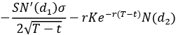
![]()
![]()

![]()
Where N() stands for the cumulative distribution function (CDF) of the Standard Normal distribution and T - t is the time to maturity expressed in years. Equation 1 represents the formula for the price of a European call option, while equation 2 represents the price of the European put option. Informally, the two terms in equation 1 can be thought of as:
- The current price of the stock, weighted by the probability of exercising the option to buy the stock (N(d1))—in other words, what we could receive
- The discounted price of exercising the option (strike), weighted by the probability of exercising the option (N(d2))—in other words, what we are going to pay
In Step 5, we used the GBM simulation function from the previous recipe to obtain 1,000,000 possible paths of the underlying asset. To calculate the option premium, we only looked at the terminal values, and for each path, calculated the payoff as follows:
- max(ST - K, 0) for the call option
- max(K - ST, 0) for the put option
In Step 6, we took the average of the payoffs and discounted it to present the value by using the discount factor.
There’s more...
Improving the valuation function using Monte Carlo simulations
In the previous steps, we showed how to reuse the GBM simulation to calculate the European call option premium. However, we can make the calculations faster, as in the case of European options we are only interested in the terminal stock price. The intermediate steps do not matter. That is why we only need to simulate the price at time T and use these values to calculate the expected payoff. We show how to do this by using an example of a European put option with the same parameters as we used before.
We start by calculating the option premium using the analytical formula:
black_scholes_analytical(S_0=S_0, K=K, T=T, r=r, sigma=sigma, type="put")
The calculated option premium is 16.9155.
Then, we define the modified simulation function, which only looks at the terminal values of the simulation paths:
def european_option_simulation(S_0, K, T, r, sigma, n_sims,
type="call", random_seed=42):
np.random.seed(random_seed)
rv = np.random.normal(0, 1, size=n_sims)
S_T = S_0 * np.exp((r - 0.5 * sigma**2) * T + sigma * np.sqrt(T) * rv)
if type == "call":
payoff = np.maximum(0, S_T - K)
elif type == "put":
payoff = np.maximum(0, K - S_T)
else:
raise ValueError("Wrong input for type!")
premium = np.mean(payoff) * np.exp(-r * T)
return premium
Then, we run the simulations:
european_option_simulation(S_0, K, T, r, sigma, N_SIMS, type="put")
The resulting value is 16.9482, which is close to the previous value. Further increasing the number of simulated paths should increase the accuracy of the valuation.
Measuring price sensitivity with the Greeks
While talking about the valuation of options, it is also worthwhile to mention the famous Greeks—quantities representing the sensitivity of the price of financial derivatives to a change in one of the underlying parameters. The name comes from the fact that those sensitivities are most commonly denoted using the letters of the Greek alphabet. The following are the five most popular sensitivities:
- Delta (
 ): The sensitivity of the theoretical option value with respect to the changes in the underlying asset’s price
 - Vega (
 ): The sensitivity of the theoretical option value with respect to the volatility of the underlying asset
 - Theta (
 ): The sensitivity of the theoretical option value with respect to the option’s time to maturity
 - Rho (
 ): The sensitivity of the theoretical option value with respect to the interest rates
 - Gamma (
 ): This is an example of a second-order Greek as it represents the sensitivity of the option’s delta (
 ) with respect to the changes in the underlying asset’s price
The following table shows how the Greeks of European call and put options are expressed in terms of the values we have already used for calculating the option’s premium using the analytical formulas:
|
What |
Calls |
Puts | |
|
delta |
|
|
|
|
gamma |
|
| |
|
vega |
|
| |
|
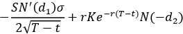
theta |
|
|
|
|
rho |
|
|
|

The N’() symbol represents the probability density function (PDF) of the Standard Normal distribution. As you can see, the Greeks are actually partial derivatives of some model price (in this case, European call or put options) with respect to one of the model’s parameters. We should also keep in mind that the Greeks differ by model.
Pricing American options with Least Squares Monte Carlo
In this recipe, we learn how to valuate American options. The key difference between European and American options is that the latter can be exercised at any time before and including the maturity date—basically, whenever the underlying asset’s price moves favorably for the option holder.
This behavior introduces additional complexity to the valuation and there is no closed-form solution to this problem. When using Monte Carlo simulations, we cannot only look at the terminal value on each sample path, as the option’s exercise can happen anywhere along the path. That is why we need to employ a more sophisticated approach called Least Squares Monte Carlo (LSMC), which was introduced by Longstaff and Schwartz (2001).
First of all, the time axis spanning [0, T] is discretized into a finite number of equally spaced intervals and the early exercise can happen only at those particular time steps. Effectively, the American option is approximated by a Bermudan one. For any time step t, the early exercise is performed in case the payoff from the immediate exercise is larger than the continuation value.
This is expressed by the following formula:
![]()
Here, ht(s) stands for the option’s payoff (also called the option’s inner value, calculated as in the case of European options) and Ct(s) is the continuation value of the option, which is defined as:
![]()
Here, r is the risk-free rate, dt is the time increment, and ![]() is the risk-neutral expectation given the underlying price. The continuation value is basically the expected payoff from not exercising the option at a given time.
is the risk-neutral expectation given the underlying price. The continuation value is basically the expected payoff from not exercising the option at a given time.
When using Monte Carlo simulations, we can define the continuation value e-rdtVt+dt,i for each path i and time t. Using this value directly is not possible as this would imply perfect foresight. That is why the LSMC algorithm uses linear regression to estimate the expected continuation value. In the algorithm, we regress the discounted future values (obtained from keeping the option) onto a set of basis functions of the spot price (time t price). The simplest way to approach this is to use an x-degree polynomial regression. Other options for the basis functions include Legendre, Hermite, Chebyshev, Gegenbauer, or Jacobi polynomials.
We iterate this algorithm backward (from time T-1 to 0) and at the last step take the average discounted value as the option premium. The premium of a European option represents the lower bound to the American option’s premium. The difference is usually called the early exercise premium.
How to do it...
Execute the following steps to price American options using the Least Squares Monte Carlo method:
- Import the libraries:
import numpy as np from chapter_10_utils import (simulate_gbm, black_scholes_analytical, lsmc_american_option) - Define the option’s parameters:
S_0 = 36 K = 40 r = 0.06 sigma = 0.2 T = 1 # 1 year N = 50 dt = T / N N_SIMS = 10 ** 5 discount_factor = np.exp(-r * dt) OPTION_TYPE = "put" POLY_DEGREE = 5 - Simulate the stock prices using a GBM:
gbm_sims = simulate_gbm(s_0=S_0, mu=r, sigma=sigma, n_sims=N_SIMS, T=T, N=N) - Calculate the payoff matrix:
payoff_matrix = np.maximum(K - gbm_sims, np.zeros_like(gbm_sims)) - Define the value matrix and fill in the last column (time T):
value_matrix = np.zeros_like(payoff_matrix) value_matrix[:, -1] = payoff_matrix[:, -1] - Iteratively calculate the continuation value and the value vector in the given time:
for t in range(N - 1, 0 , -1): regression = np.polyfit( gbm_sims[:, t], value_matrix[:, t + 1] * discount_factor, POLY_DEGREE ) continuation_value = np.polyval(regression, gbm_sims[:, t]) value_matrix[:, t] = np.where( payoff_matrix[:, t] > continuation_value, payoff_matrix[:, t], value_matrix[:, t + 1] * discount_factor ) - Calculate the option’s premium:
option_premium = np.mean(value_matrix[:, 1] * discount_factor)
option_premium
The premium on the specified American put option is
4.465.
- Calculate the premium of a European put with the same parameters:
black_scholes_analytical(S_0=S_0, K=K, T=T, r=r, sigma=sigma,
                         type="put")
The price of the European put option with the same parameters is
3.84.
- As an extra check, calculate the prices of the American and European call options:
european_call_price = black_scholes_analytical(
    S_0=S_0, K=K, T=T, r=r, sigma=sigma
)
american_call_price = lsmc_american_option(
    S_0=S_0, K=K, T=T, N=N, r=r,
    sigma=sigma, n_sims=N_SIMS,
    option_type="call",
    poly_degree=POLY_DEGREE
)
print(f"European call's price: {european_call_price:.3f}")
print(f"American call's price: {american_call_price:.3f}")
The price of the European call is 2.17, while the American call’s price (using 100,000 simulations) is 2.10.
How it works...
In Step 2, we once again defined the parameters of the considered American option. For comparison’s sake, we took the same values that Longstaff and Schwartz (2001) did. In Step 3, we simulated the stock’s evolution using the simulate_gbm function from the previous recipe. Afterward, we calculated the payoff matrix of the put option using the same formula that we used for the European options.
In Step 5, we prepared the matrix of option values over time, which we defined as a matrix of zeros of the same size as the payoff matrix. We filled the last column of the value matrix with the last column of the payoff matrix, as at the last step there are no further computations to carry out—the payoff is equal to the European option.
In Step 6, we ran the backward part of the algorithm from time T-1 to 0. At each of these steps, we estimated the expected continuation value as a cross-sectional linear regression. We fitted the 5th-degree polynomial to the data using np.polyfit.
Then, we evaluated the polynomial at specific values (using np.polyval), which is the same as getting the fitted values from a linear regression. We compared the expected continuation value to the payoff to see if the option should be exercised. If the payoff was higher than the expected value from continuation, we set the value to the payoff. Otherwise, we set it to the discounted one-step-ahead value. We used np.where for this selection.
It is also possible to use scikit-learn for the polynomial fit. To do so, you need to combine LinearRegression with PolynomialFeatures.
In Step 7 of the algorithm, we obtained the option premium by taking the average value of the discounted t = 1 value vector.
In the last two steps, we carried out some sanity checks. First, we calculated the premium of a European put with the same parameters. Second, we repeated all the steps to get the premiums of American and European call options with the same parameters. To make this easier, we put the entire algorithm for LSMC into one function, which is available in this book’s GitHub repository.
For the call option, the premium on the American and European options should be equal, as it is never optimal to exercise the option when there are no dividends. Our results are very close, but we can obtain a more accurate price by increasing the number of simulated sample paths.
In principle, the Longstaff-Schwartz algorithm should underprice American options because the approximation of the continuation value by the basis functions is just that, an approximation. As a consequence, the algorithm will not always make the correct decision about exercising the option. This, in turn, means that the option’s value will be lower than in the case of the optimal exercise.
See also
Additional resources are available here:
- Longstaff, F. A., & Schwartz, E. S. 2001. “Valuing American options by simulation: a simple least-squares approach,” The Review of Financial Studies, 14(1): 113-147
- Broadie, M., Glasserman, P., & Jain, G. 1997. “An alternative approach to the valuation of American options using the stochastic tree method. Enhanced Monte Carlo estimates for American option prices,” Journal of Derivatives, 5: 25-44.
Pricing American options using QuantLib
In the previous recipe, we showed how to manually code the Longstaff-Schwartz algorithm. However, we can also use already existing frameworks for the valuation of derivatives. One of the most popular ones is QuantLib. It is an open-source C++ library that provides tools for the valuation of financial instruments. By using Simplified Wrapper and Interface Generator (SWIG), it is possible to use QuantLib from Python (and some other programming languages, such as R or Julia). In this recipe, we show how to price the same American put option that we priced in the previous recipe, but the library itself has many more interesting features to explore.
Getting ready
Execute Step 2 from the previous recipe to have the parameters of the American put option that we will valuate using QuantLib.
How to do it...
Execute the following steps to price American options using QuantLib:
- Import the library:
import QuantLib as ql - Specify the calendar and the day-counting convention:
calendar = ql.UnitedStates() day_counter = ql.ActualActual() - Specify the valuation date and the expiry date of the option:
valuation_date = ql.Date(1, 1, 2020) expiry_date = ql.Date(1, 1, 2021) ql.Settings.instance().evaluationDate = valuation_date - Define the option type (call/put), type of exercise (American), and payoff:
if OPTION_TYPE == "call": option_type_ql = ql.Option.Call elif OPTION_TYPE == "put": option_type_ql = ql.Option.Put exercise = ql.AmericanExercise(valuation_date, expiry_date) payoff = ql.PlainVanillaPayoff(option_type_ql, K) - Prepare the market-related data:
u = ql.SimpleQuote(S_0) r = ql.SimpleQuote(r) sigma = ql.SimpleQuote(sigma) - Specify the market-related curves:
underlying = ql.QuoteHandle(u) volatility = ql.BlackConstantVol(0, ql.TARGET(), ql.QuoteHandle(sigma), day_counter) risk_free_rate = ql.FlatForward(0, ql.TARGET(), ql.QuoteHandle(r), day_counter) - Plug the market-related data into the Black-Scholes process:
bs_process = ql.BlackScholesProcess( underlying, ql.YieldTermStructureHandle(risk_free_rate), ql.BlackVolTermStructureHandle(volatility), ) - Instantiate the Monte Carlo engine for the American options:
engine = ql.MCAmericanEngine( bs_process, "PseudoRandom", timeSteps=N, polynomOrder=POLY_DEGREE, seedCalibration=42, requiredSamples=N_SIMS ) - Instantiate the
optionobject and set its pricing engine:option = ql.VanillaOption(payoff, exercise) option.setPricingEngine(engine) - Calculate the option’s premium:
option_premium_ql = option.NPV()
option_premium_ql
The value of the American put option is 4.457.
How it works...
Since we wanted to compare the results we obtained with those in the previous recipes, we used the same problem setup as we did there. For brevity, we will not look at all the code here, but we should run Step 2 from the previous recipe.
In Step 2, we specified the calendar and the day-counting convention. The day-counting convention determines the way interest accrues over time for various financial instruments, such as bonds. The actual/actual convention means that we use the actual number of elapsed days and the actual number of days in a year, that is, 365 or 366. There are many other conventions such as actual/365 (fixed), actual/360, and so on.
In Step 3, we selected two dates—valuation and expiry—as we are interested in pricing an option that expires in a year. It is important to set ql.Settings.instance().evaluationDate to the considered evaluation date to make sure the calculations are performed correctly. In this case, the dates only determine the passage of time, meaning that the option expires within a year. We would get the same results (with some margin of error due to the random component of the simulations) using different dates with the same interval between them.
We can check the time to expiry (in years) by running the following code:
T = day_counter.yearFraction(valuation_date, expiry_date)
print(f'Time to expiry in years: {T}')
Executing the snippet returns the following:
Time to expiry in years: 1.0
Next, we defined the option type (call/put), the type of exercise (European, American, or Bermudan), and the payoff (vanilla). In Step 5, we prepared the market data. We wrapped the values in quotes (ql.SimpleQuote) so that the values can be changed and those changes are properly registered in the instrument. This is an important step for calculating the Greeks in the There’s more… section.
In Step 6, we defined the relevant curves. Simply put, TARGET is a calendar that contains information on which days are holidays.
In this step, we specified the three important components of the Black-Scholes (BS) process, which are:
- The price of the underlying instrument
- Volatility, which is constant as per our assumptions
- The risk-free rate, which is also constant over time
We passed all these objects to the Black-Scholes process (ql.BlackScholesProcess), which we defined in Step 7. Then, we passed the process object into the special engine used for pricing American options using Monte Carlo simulations (there are many predefined engines for different types of options and pricing methods). At this point, we provided the desired number of simulations, the number of time steps for discretization, and the degree/order of the polynomial in the LSMC algorithm. Additionally, we provided the random seed (seedCalibration) to make the results reproducible.
In Step 9, we created an instance of ql.VanillaOption by providing previously defined types of payoff and exercise. We also set the pricing engine to the one defined in Step 8 using the setPricingEngine method.
Finally, we obtained the price of the option using the NPV method.
We can see that the option premium we obtained using QuantLib is very similar to the one we calculated previously, which further validates our results. The important thing to note here is that the workflow is similar for the valuation of a wide array of different derivatives, so it is good to be familiar with it. We could just as well price a European option using Monte Carlo simulations by substituting a few classes with their European option counterparts.
QuantLib also allows us to use variance reduction techniques such as antithetic values or control variates.
There’s more...
Now that we have completed the preceding steps, we can calculate the Greeks. As we have mentioned in the previous recipe, the Greeks represent the sensitivity of the price of derivatives to a change in one of the underlying parameters (such as the price of the underlying asset, time to expiry, and so on).
When there is an analytical formula available for the Greeks (when the underlying QuantLib engine is using analytical formulas), we could just access it by running, for example, option.delta(). However, in cases such as valuations using binomial trees or simulations, there is no analytical formula, and we would receive an error (RuntimeError: delta not provided). This does not mean that it is impossible to calculate it, but we need to employ numerical differentiation and calculate it ourselves.
In this example, we will only extract the delta. Therefore, the relevant two-sided formula is:

Here, P(S) is the price of the instrument given the underlying asset’s price S; h is a very small increment.
Run the following block of code to calculate the delta:
u_0 = u.value() # original value
h = 0.01
u.setValue(u_0 + h)
P_plus_h = option.NPV()
u.setValue(u_0 - h)
P_minus_h = option.NPV()
u.setValue(u_0) # set back to the original value
delta = (P_plus_h - P_minus_h) / (2 * h)
The simplest interpretation of the delta is that the option’s delta equal to -1.36 indicates that, if the underlying stock increases in price by $1 per share, the option on it will decrease by $1.36 per share; otherwise, everything will be equal.
Pricing barrier options
A barrier option is a type of option that falls under the umbrella of exotic options. That is because they are more complex than plain European or American options. Barrier options are a type of path-dependent option because their payoff, and thus also their value, is based on the underlying asset’s price path.
To be more precise, the payoff depends on whether or not the underlying asset has reached/exceeded a predetermined price threshold. Barrier options are typically classified as one of the following:
- A knock-out option, that is, the option becomes worthless if the underlying asset’s price exceeds a certain threshold
- A knock-in option, that is, the option has no value until the underlying asset’s price reaches a certain threshold
Considering the classes of the barrier options mentioned above, we can deal with the following categories:
- Up-and-Out: The option starts active and becomes worthless (knocked out) when the underlying asset’s price moves up to the barrier level
- Up-and-In: The option starts inactive and becomes active (knocked in) when the underlying asset’s price moves up to the barrier level
- Down-and-Out: The option starts active and becomes knocked out when the underlying asset’s price moves down to the barrier level
- Down-and-In: The option starts inactive and becomes active when the underlying asset’s price moves down to the barrier level
Other than the behavior described above, barrier options behave like standard call and put options.
In this recipe, we use Monte Carlo simulations to price an Up-and-In European call option with the underlying trading at $55, a strike price of $60, and a barrier level of $65. The time to maturity will be 1 year.
How to do it…
Execute the following steps to price an Up-and-In European call option:
- Import the libraries:
import numpy as np from chapter_10_utils import simulate_gbm - Define the parameters for the valuation:
S_0 = 55 K = 60 BARRIER = 65 r = 0.06 sigma = 0.2 T = 1 N = 252 dt = T / N N_SIMS = 10 ** 5 OPTION_TYPE = "call" discount_factor = np.exp(-r * T) - Simulate the stock path using the
simulate_gbmfunction:gbm_sims = simulate_gbm(s_0=S_0, mu=r, sigma=sigma, n_sims=N_SIMS, T=T, N=N) - Calculate the maximum value per path:
max_value_per_path = np.max(gbm_sims, axis=1) - Calculate the payoff:
payoff = np.where(max_value_per_path > BARRIER, np.maximum(0, gbm_sims[:, -1] - K), 0) - Calculate the option’s premium:
premium = discount_factor * np.mean(payoff)
premium
The premium of the considered Up-and-In European call option is 3.6267.
How it works…
In the first two steps, we imported the libraries (including the helper function, simulate_gbm, which we have already used throughout this chapter) and defined the parameters of the valuation.
In Step 3, we simulated 100,000 possible paths using a geometric Brownian motion. Then, we calculated the maximum price of the underlying asset for each path. Because we are working with an Up-and-In option, we just need to know if the maximum price of the asset reached the barrier level. If so, then the option’s payoff at maturity will be equal to that of a vanilla European call. If the barrier level was not reached, the payoff from that path will be zero. We encoded that payoff condition in Step 5.
Lastly, we proceeded just as we have done with the European call option before—we took the average payoff and discounted it using the discount factor.
We can build some intuition about the prices of barrier options. For example, the price of an Up-and-Out barrier option should be lower than that of a vanilla equivalent. That is due to the fact that the payoffs of the two instruments would be identical except for the added risk that the Up-and-Out barrier option could be knocked-out before expiring. That added risk should be reflected in the lower price of such a barrier option as compared to its vanilla counterpart.
In this recipe, we have manually priced an Up-and-In European call option. However, we can also use the QuantLib library for the task. Due to the fact that there would be a lot of code repetition with the previous recipe, we do not show that in the book.
But you are highly encouraged to check out the solution using QuantLib in the accompanying notebook available on GitHub. We just mention that the solution using QuantLib returns the option premium of 3.6457, which is very close to the one we obtained manually. The difference can be attributed to the random component of the simulations.
There’s more…
The valuation of barrier options is complex given those instruments are path-dependent. We have already mentioned how to use Monte Carlo simulations to price such options; however, there are several alternative approaches:
- Use a static replicating portfolio of vanilla options to mimic the value of the barrier at expiry and at a few discrete points in time along the barrier. Then, those options can be valued using the Black-Scholes model. By following this approach, we can obtain closed-form prices and replication strategies for all kinds of barrier options.
- Use the binomial tree approach to option pricing.
- Use the partial differential equation (PDE) and potentially combine it with the finite difference method.
Estimating Value-at-Risk using Monte Carlo
Value-at-Risk (VaR) is a very important financial metric that measures the risk associated with a position, portfolio, etc. It is commonly abbreviated to VaR, not to be confused with vector autoregression (which is abbreviated to VAR). VaR reports the worst expected loss—at a given level of confidence—over a certain horizon under normal market conditions. The easiest way to understand it is by looking at an example. Let’s say that the 1-day 95% VaR of our portfolio is $100. This means that 95% of the time (under normal market conditions), we will not lose more than $100 by holding our portfolio over one day.
It is common to present the loss given by VaR as a positive (absolute) value. That is why in this example, a VaR of $100 means losing no more than $100. However, a negative VaR is possible and it would indicate a high probability of making a profit. For example, a 1-day 95% VaR of $-100 would imply that our portfolio has a 95% chance of making more than $100 over the next day.
There are several ways to calculate VaR, including:
- Parametric approach (variance-covariance)
- Historical simulation approach
- Monte Carlo simulations
In this recipe, we only consider the last method. We assume that we are holding a portfolio consisting of two assets (stocks of Intel and AMD) and that we want to calculate a 1-day Value-at-Risk.
How to do it...
Execute the following steps to estimate the Value-at-Risk using Monte Carlo simulations:
- Import the libraries:
import numpy as np import pandas as pd import yfinance as yf import seaborn as sns - Define the parameters that will be used for this recipe:
RISKY_ASSETS = ["AMD", "INTC"] SHARES = [5, 5] START_DATE = "2020-01-01" END_DATE = "2020-12-31" T = 1 N_SIMS = 10 ** 5 - Download the price data from Yahoo Finance:
df = yf.download(RISKY_ASSETS, start=START_DATE, end=END_DATE, adjusted=True) - Calculate the daily returns:
returns = df["Adj Close"].pct_change().dropna()
returns.plot(title="Intel's and AMD's daily stock returns in 2020")
Running the snippet results in the following figure.
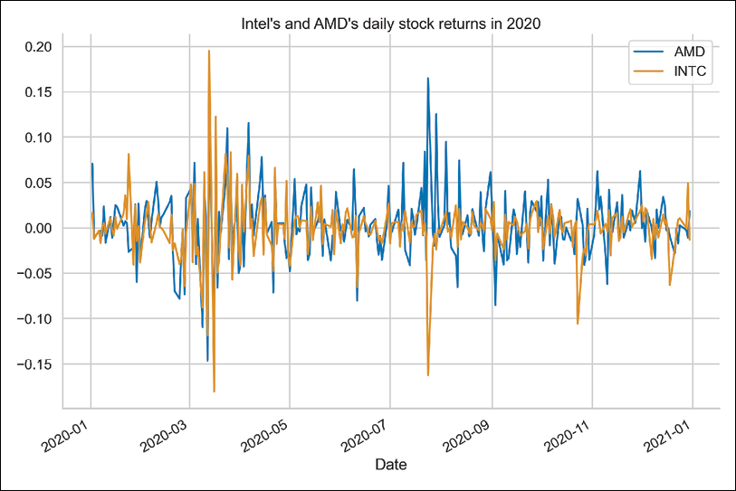
Figure 10.3: Simple returns of Intel and AMD in 2020
Additionally, we calculated the Pearson’s correlation between the two series (using the
corrmethod), which is equal to0.5.
- Calculate the covariance matrix:
cov_mat = returns.cov() - Perform the Cholesky decomposition of the covariance matrix:
chol_mat = np.linalg.cholesky(cov_mat) - Draw the correlated random numbers from the Standard Normal distribution:
rv = np.random.normal(size=(N_SIMS, len(RISKY_ASSETS))) correlated_rv = np.transpose( np.matmul(chol_mat, np.transpose(rv)) ) - Define the metrics that will be used for simulations:
r = np.mean(returns, axis=0).values sigma = np.std(returns, axis=0).values S_0 = df["Adj Close"].values[-1, :] P_0 = np.sum(SHARES * S_0) - Calculate the terminal price of the considered stocks:
S_T = S_0 * np.exp((r - 0.5 * sigma ** 2) * T + sigma * np.sqrt(T) * correlated_rv) - Calculate the terminal portfolio value and the portfolio returns:
P_T = np.sum(SHARES * S_T, axis=1) P_diff = P_T - P_0 - Calculate the VaR for the selected confidence levels:
P_diff_sorted = np.sort(P_diff)
percentiles = [0.01, 0.1, 1.]
var = np.percentile(P_diff_sorted, percentiles)
for x, y in zip(percentiles, var):
    print(f'1-day VaR with {100-x}% confidence: ${-y:.2f}')
Running the snippet results in the following output:
1-day VaR with 99.99% confidence: $2.04
1-day VaR with 99.9% confidence: $1.48
1-day VaR with 99.0% confidence: $0.86
- Present the results on a graph:
ax = sns.distplot(P_diff, kde=False)
ax.set_title("""Distribution of possible 1-day changes
              in portfolio value 1-day 99% VaR""",
              fontsize=16)
ax.axvline(var[2], 0, 10000)
Running the snippet results in the following figure:
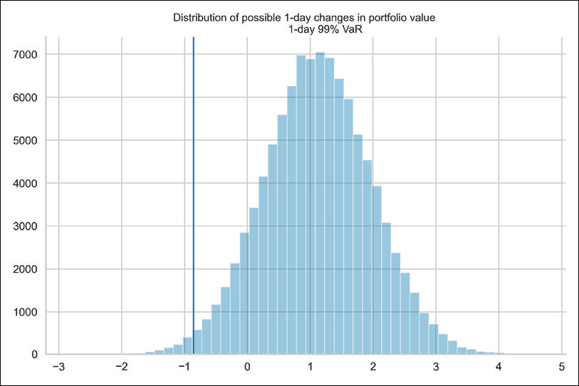
Figure 10.4: Distribution of the possible 1-day changes in portfolio value and the 1-day 99% VaR
Figure 10.4 shows the distribution of possible 1-day-ahead portfolio values. We present the 99% Value-at-Risk with the vertical line.
How it works...
In Steps 2 to 4, we downloaded the daily stock prices of Intel and AMD from the year 2020, extracted the adjusted close prices, and converted them into simple returns. We also defined a few parameters, such as the number of simulations and the number of shares we have in our portfolio.
There are two ways to approach VaR calculations:
- Calculate VaR from prices: Using the number of shares and the asset prices, we can calculate the worth of the portfolio now and its possible value X days ahead.
- Calculate VaR from returns: Using the percentage weights of each asset in the portfolio and the assets’ expected returns, we can calculate the expected portfolio return X days ahead. Then, we can express VaR as the dollar amount based on that return and the current portfolio value.
The Monte Carlo approach to determining the price of an asset employs random variables drawn from the Standard Normal distribution. For the case of calculating portfolio VaR, we need to account for the fact that the assets in our portfolio may be correlated. To do so, in Steps 5 to 7, we generated correlated random variables. To do so, we first calculated the historical covariance matrix. Then, we used the Cholesky decomposition on it and multiplied the resulting matrix by the matrix containing the random variables.
Another possible approach to making random variables correlated is to use the Singular Value Decomposition (SVD) instead of the Cholesky decomposition. The function we can use for this is np.linalg.svd.
In Step 8, we calculated metrics such as the historical averages of the asset return, the accompanying standard deviations, the last known stock prices, and the initial portfolio value. In Step 9, we applied the analytical solution to the geometric Brownian motion SDE and calculated possible 1-day-ahead stock prices for both assets.
To calculate the portfolio VaR, we calculated the possible 1-day-ahead portfolio values and the accompanying differences (PT - P0). Then, we sorted them in ascending order. The X% VaR is simply the (1-X)-th percentile of the sorted portfolio differences.
Banks frequently calculate the 1-day and 10-day VaR. To arrive at the latter, they can simulate the value of their assets over a 10-day interval using 1-day steps (discretization). However, they can also calculate the 1-day VaR and multiply it by the square root of 10. This might be beneficial for the bank if it leads to lower capital requirements.
There’s more...
As we have mentioned, there are multiple ways of calculating the Value-at-Risk. And each of those comes with a set of potential drawbacks, some of which are:
- Assuming a parametric distribution (variance-covariance approach)
- Assuming that daily gains/losses are IID (independently and identically distributed)
- Not capturing enough tail risk
- Not considering the so-called Black Swan events (unless they are already in the historical sample)
- Historical VaR can be slow to adapt to new market conditions
- The historical simulation approach assumes that past returns are sufficient to evaluate future risk (connects to the previous points)
There are some interesting recent developments in using deep learning techniques, for example, generative adversarial networks for Value-at-Risk estimation.
Another general drawback of VaR is that it does not contain information about the size of the potential loss when it exceeds the threshold given by VaR. This is when expected shortfall (also known as conditional VaR or expected tail loss) comes into play. It simply states what the expected loss is in the worst X% of scenarios.
There are many ways to calculate the Expected Shortfall, but we present the one that is easily connected to the VaR and can be estimated using Monte Carlo simulations.
Following on from the example of a two-asset portfolio, we would like to know the following: if the loss exceeds the VaR, how big will it be? To obtain that number, we need to filter out all losses that are higher than the value given by VaR and calculate their expected value by taking the average.
We can do this using the following snippet:
var = np.percentile(P_diff_sorted, 5)
expected_shortfall = P_diff_sorted[P_diff_sorted<=var].mean()
Please bear in mind that for Expected Shortfall we only use a small fraction of all the simulations that were used to obtain the VaR. In Figure 10.4, we would only consider the observations to the left of the VaR line. That is why, in order to have reasonable results for the Expected Shortfall, the overall sample must be large enough.
The 1-day 95% VaR is $0.29, while the accompanying Expected Shortfall is $0.64. We can interpret these results as follows: if the loss exceeds the 95% VaR, we can expect to lose $0.64 by holding our portfolio for 1 day.
Summary
In this chapter, we have covered Monte Carlo simulations, which are a very versatile tool useful in many financial tasks. We demonstrated how to utilize them for simulating stock prices using a geometric Brownian motion, pricing various types of options (European, American, and Barrier), and calculating the Value-at-Risk.
However, in this chapter we have barely scratched the surface of all the possible applications of Monte Carlo simulations. In the following chapter, we also show how to use them to obtain the efficient frontier used for asset allocation.
Join us on Discord!
To join the Discord community for this book – where you can share feedback, ask questions to the author, and learn about new releases – follow the QR code below: