12
Backtesting Trading Strategies
In the previous chapters, we gained the knowledge necessary to create trading strategies. On the one hand, we could use technical analysis to identify trading opportunities. On the other, we could use some of the other techniques we have already covered in the book. We could try to use knowledge about factor models or volatility forecasting. Or, we could use portfolio optimization techniques to determine the optimal quantity of assets for our investment. One crucial thing that is still missing is evaluating how such a strategy would have performed if we had implemented it in the past. That is the goal of backtesting, which we explore in this chapter.
Backtesting can be described as a realistic simulation of our trading strategy, which assesses its performance using historical data. The underlying idea is that the backtest performance should be indicative of future performance when the strategy is actually used on the market. Naturally, this will not always be the case and we should keep that in mind when experimenting.
There are multiple ways of approaching backtesting, however, we should always remember that a backtest should faithfully represent how markets operate, how trades are executed, what orders are available, and so on. For example, forgetting to account for transaction costs can quickly turn a “profitable” strategy into a failed experiment.
We have already mentioned the generic uncertainty around predictions in the ever-changing financial markets. However, there are also some implementation aspects that can bias the results of backtests and increase the risk of confusing in-sample performance with generalizable patterns that will also hold out of sample. We briefly mention some of those below:
- Look-ahead bias: This potential flaw emerges when we develop a trading strategy using historical data before it was actually known/available. Some examples include corrections of reported financial statements after their publication, stock splits, or reverse splits.
- Survivorship bias: This bias arises when we backtest only using data about securities that are currently active/tradeable. By doing so, we omit the assets that have disappeared over time (due to bankruptcy, delisting, acquisition, and so on). Most of the time, those assets did not perform well and our strategies can be skewed by failing to include those, as those assets could have been picked up in the past when they were still available in the markets.
- Outlier detection and treatment: The main challenge is to discern the outliers that are not representative of the analyzed period as opposed to the ones that are an integral part of the market behavior.
- Representative sample period: As the goal of the backtest is to provide an indication of future performance, the sample data should reflect the current, and potentially also future, market behavior. By not spending enough time on this part, we can miss some crucial market regime aspects such as volatility (too few/many extreme events) or volume (too few data points).
- Meeting investment objectives and constraints over time: It can happen that a strategy leads to good performance at the very end of the evaluation period. However, in some periods when it was active, it resulted in unacceptably high losses or volatility. We could potentially track those by using rolling performance/risk metrics, for example, the value-at-risk or the Sharpe/Sortino ratio.
- Realistic trading environment: We have already mentioned that failing to include transaction costs can greatly impact the end result of a backtest. What is more, real-life trading involves further complications. For example, it might not be possible to execute all trades at all times or at the target price. Some of the things to consider are slippage (the difference between the expected price of a trade and the price at which the trade is executed), the availability of a counterparty for short positions, broker fees, and so on. The realistic environment also accounts for the fact that we might make a trading decision based on the close prices of one day, but the trade will be (potentially) executed based on the open prices of the next trading day. It can happen that the order we prepare will not be executed due to large price differences.
- Multiple testing: When running multiple backtests, we might discover spurious results or a strategy that overfits the test sample and produces suspiciously positive results that are unlikely to hold for out-of-sample data encountered during live trading. Also, we might leak prior knowledge of what works and what does not into the design of strategies, which can lead to further overfitting. Some things that we can consider are: reporting the number of trials, calculating the minimum backtest length, using some sort of optimal stopping rule, or calculating metrics that account for the effect of multiple testing (for example, the deflated Sharpe ratio).
In this chapter, we show how to run backtests of various trading strategies using two approaches: vectorized and event-driven. We will go into the details of each of the approaches later on, but now we can state that the first one works well for a quick test to see if there is any potential in the strategy. On the other hand, the latter is more suited for thorough and rigorous testing, as it tries to account for many of the potential issues mentioned above.
The key learning of this chapter is how to set up a backtest using popular Python libraries. We will be showing a few examples of strategies built on the basis of popular technical indicators or a strategy using mean-variance portfolio optimization. With that knowledge, you can backtest any strategy you can come up with.
We present the following recipes in this chapter:
- Vectorized backtesting with pandas
- Event-driven backtesting with backtrader
- Backtesting a long/short strategy based on the RSI
- Backtesting a buy/sell strategy based on Bollinger bands
- Backtesting a moving average crossover strategy using crypto data
- Backtesting a mean-variance portfolio optimization
Vectorized backtesting with pandas
As we mentioned in the introduction to this chapter, there are two approaches to carrying out backtests. The simpler one is called vectorized backtesting. In this approach, we multiply a signal vector/matrix (containing an indicator of whether we are entering or closing a position) by the vector of returns. By doing so, we calculate the performance over a certain period of time.
Due to its simplicity, this approach cannot deal with many of the issues we described in the introduction, for example:
- We need to manually align the timestamps to avoid look-ahead bias.
- There is no explicit position sizing.
- All performance measurements are calculated manually at the very end of the backtest.
- Risk-management rules like stop-loss are not easy to incorporate.
That is why we should use vectorized backtesting mostly if we are dealing with simple trading strategies and want to explore their initial potential in a few lines of code.
In this recipe, we backtest a very simple strategy with the following set of rules:
- We enter a long position if the close price is above the 20-day Simple Moving Average (SMA)
- We close the position when the close price goes below the 20-day SMA
- Short selling is not allowed
- The strategy is unit agnostic (we can enter a position of 1 share or 1000 shares) because we only care about the percentage change in the prices
We backtest this strategy using Apple’s stock and its historical prices from the years 2016 to 2021.
How to do it…
Execute the following steps to backtest a simple strategy using the vectorized approach:
- Import the libraries:
import pandas as pd import yfinance as yf import numpy as np - Download Apple’s stock prices from the years 2016 to 2021 and keep only the adjusted close price:
df = yf.download("AAPL", start="2016-01-01", end="2021-12-31", progress=False) df = df[["Adj Close"]] - Calculate the log returns and the 20-day SMA of the close prices:
df["log_rtn"] = df["Adj Close"].apply(np.log).diff(1) df["sma_20"] = df["Adj Close"].rolling(window=20).mean() - Create a position indicator:
df["position"] = (df["Adj Close"] > df["sma_20"]).astype(int)Using the following snippet, we count how many times we entered a long position:
sum((df["position"] == 1) & (df["position"].shift(1) == 0))The answer is 56.
- Visualize the strategy over 2021:
fig, ax = plt.subplots(2, sharex=True)
df.loc["2021", ["Adj Close", "sma_20"]].plot(ax=ax[0])
df.loc["2021", "position"].plot(ax=ax[1])
ax[0].set_title("Preview of our strategy in 2021")
Executing the snippet generates the following figure:

Figure 12.1: The preview of our trading strategy based on the simple moving average
In Figure 12.1, we can clearly see how our strategy works—in the periods when the close price is above the 20-day SMA, we do have an open position. This is indicated by the value of 1 in the column containing the position information.
- Calculate the strategy’s daily and cumulative returns:
df["strategy_rtn"] = df["position"].shift(1) * df["log_rtn"] df["strategy_rtn_cum"] = ( df["strategy_rtn"].cumsum().apply(np.exp) ) - Add the buy-and-hold strategy for comparison:
df["bh_rtn_cum"] = df["log_rtn"].cumsum().apply(np.exp) - Plot the strategies’ cumulative returns:
(
    df[["bh_rtn_cum", "strategy_rtn_cum"]]
    .plot(title="Cumulative returns")
)
Executing the snippet generates the following figure:

Figure 12.2: The cumulative returns of our strategy and the buy-and-hold benchmark
In Figure 12.2, we can see the cumulative returns of both strategies. The initial conclusion could be that the simple strategy outperformed the buy-and-hold strategy over the considered time period. However, this form of a simplified backtest does not consider quite a lot of crucial aspects (for example, trading using the close price, it assumes lack of slippage and transaction costs, and so on) that can dramatically change the final outcome. In the There’s more... section, we will see how quickly the results change when we account for transaction costs alone.
How it works…
At the very beginning, we imported the libraries and downloaded Apple’s stock prices from the years 2016 to 2021. We only kept the adjusted close price for the backtest.
In Step 3, we calculated the log returns and the 20-day SMA. To calculate the technical indicator, we used the rolling method of a pandas DataFrame. However, we could have just as well used the already explored TA-Lib library.
We calculated the log returns, as they have a convenient property of summing up over time. If we held the position for 10 days and are interested in the final return of the position, we can simply sum up the log returns from those 10 days. For more information, please refer to Chapter 2, Data Preprocessing.
In Step 4, we created a column with information on whether we have an open position (long only) or not. As we have decided, we enter the position when the close price is above the 20-day SMA. We exit the position when the close price goes below the SMA. We have also encoded this column in the DataFrame as an integer. In Step 5, we plotted the close price, the 20-day SMA, and the column with the position flag. To make the plot more readable, we only plotted the data from 2021.
Step 6 is the most important one in the vectorized backtest. There, we calculated the strategy’s daily and cumulative returns. To calculate the daily return, we multiplied the log return of that day with the shifted position flag. The position vector is shifted by 1 to avoid the look-ahead bias. In other words, the flag is generated using all the information up to and including time t. We can only use that information to open a position on the next trading day, that is, at time t+1.
An inquisitive reader might already spot another bias that is occurring with our backtest. We are correctly assuming that we can only buy on the next trading day, however, the log return is calculated as we have bought on day t+1 using the close price of time t, which can be very untrue depending on the market conditions. We will see how to overcome this issue with event-driven backtesting in the next recipes.
Then, we used the cumsum method to calculate the cumulative sum of the log returns, which corresponds to the cumulative return. Lastly, we applied the exponent function using the apply method.
In Step 7, we calculated the cumulative returns of a buy-and-hold strategy. For this one, we simply used the log returns for the calculations, skipping the step in which we multiplied the returns with the position flag.
In the last step, we plotted the cumulative returns of both strategies.
There’s more...
From the initial backtest, it seems that the simple strategy is outperforming the buy-and-hold strategy. But we have also seen that over the 6 years, we have entered a long position 56 times. The total number of trades doubles, as we also exited those positions. Depending on the broker, this can result in quite significant transaction costs.
Given that transaction costs are frequently quoted in fixed percentages, we can simply calculate by how much the portfolio has changed between successive time steps, calculate the transaction costs on that basis, and then subtract them directly from our strategy’s returns.
In the steps below, we show how to account for the transaction costs in a vectorized backtest. For simplicity, we assume that the transaction costs are 1%.
Execute the following steps to account for transaction costs in the vectorized backtest:
- Calculate daily transaction costs:
TRANSACTION_COST = 0.01
df["tc"] = df["position"].diff(1).abs() * TRANSACTION_COST
In this snippet, we calculated if there is a change in our portfolio (absolute value, as we can enter or exit a position) and then multiplied that value by the transaction costs expressed as a percentage.
- Calculate the strategy’s performance accounting for transaction costs:
df["strategy_rtn_cum_tc"] = ( (df["strategy_rtn"] - df["tc"]).cumsum().apply(np.exp) ) - Plot the cumulative returns of all the strategies:
STRATEGY_COLS = ["bh_rtn_cum", "strategy_rtn_cum",
                 "strategy_rtn_cum_tc"]
(
    df
    .loc[:, STRATEGY_COLS]
    .plot(title="Cumulative returns")
)
Executing the snippet generates the following figure:

Figure 12.3: Cumulative returns of all strategies, including the one with transaction costs
After accounting for transaction costs, the performance decreased significantly and is worse than that of the buy-and-hold. And to be entirely fair, we should also account for the initial and terminal transaction costs in the buy-and-hold strategy, as we had to buy and sell the asset once.
Event-driven backtesting with backtrader
The second approach to backtesting is called event-driven backtesting. In this approach, a backtesting engine simulates the time dimension of the trading environment (you can think about it as a for loop going through the time and executing all the actions sequentially). This imposes more structure on the backtest, including the use of historical calendars to define when trades can actually be executed, when prices are available, and so on.
Event-driven backtesting aims to simulate all the actions and constraints encountered when executing a certain strategy while allowing for much more flexibility than the vectorized approach. For example, this approach allows for simulating potential delays in orders’ execution, slippage costs, and so on. In an ideal scenario, a strategy encoded for an event-driven backtest could be easily converted into one working with live trading engines.
Nowadays, there are quite a few event-driven backtesting libraries available for Python. In this chapter, we introduce one of the most popular ones—backtrader. Key features of this framework include:
- A vast amount of available technical indicators (
backtraderalso provides a wrapper around the popular TA-Lib library) and performance measures. - Ease of building and applying new indicators.
- Multiple data sources are available (including Yahoo Finance and Nasdaq Data Link), with the possibility to load external files.
- Simulating many aspects of real brokers, such as different types of orders (market, limit, and stop), slippage, commission, going long/short, and so on.
- Comprehensive and interactive visualization of the prices, TA indicators, trading signals, performance, and so on.
- Live trading with selected brokers.
For this recipe, we consider a basic strategy based on the simple moving average. As a matter of fact, it is almost identical to the one we backtested in the previous recipe using the vectorized approach. The logic of the strategy is as follows:
- When the close price becomes higher than the 20-day SMA, buy one share.
- When the close price becomes lower than the 20-day SMA and we have a share, sell it.
- We can only have a maximum of one share at any given time.
- No short selling is allowed.
We run the backtesting of this strategy using Apple’s stock prices from the year 2021.
Getting ready
In this recipe (and in the rest of the chapter), we will be using two helper functions used for printing logs—get_action_log_string and get_result_log_string. Additionally, we will use a custom MyBuySell observer to display the position markers in different colors. You can find the definitions of those helpers in the strategy_utils.py file available on GitHub.
At the time of writing, the version of backtrader available at PyPI (the Python Package Index) is not the latest. Installing with a simple pip install backtrader command will install a version containing quite a few issues, for example, with loading the data from Yahoo Finance. To overcome this, you should install the latest version from GitHub. You can do so using the following snippet:
pip install git+https://github.com/mementum/backtrader.git#egg=backtrader
How to do it...
Execute the following steps to backtest a simple strategy using the event-driven approach:
- Import the libraries:
from datetime import datetime import backtrader as bt from backtrader_strategies.strategy_utils import * - Download data from Yahoo Finance:
data = bt.feeds.YahooFinanceData(dataname="AAPL",
                                 fromdate=datetime(2021, 1, 1),
                                 todate=datetime(2021, 12, 31))
To make the code more readable, we first present the general outline of the class defining the trading strategy and then introduce the separate methods in the following substeps.
- The template of the strategy is presented below:
class SmaStrategy(bt.Strategy): params = (("ma_period", 20), ) def __init__(self): # some code def log(self, txt): # some code def notify_order(self, order): # some code def notify_trade(self, trade): # some code def next(self): # some code def start(self): # some code def stop(self): # some code- The
__init__method is defined as:def __init__(self): # keep track of close price in the series self.data_close = self.datas[0].close # keep track of pending orders self.order = None # add a simple moving average indicator self.sma = bt.ind.SMA(self.datas[0], period=self.params.ma_period) - The
logmethod is defined as:def log(self, txt): dt = self.datas[0].datetime.date(0).isoformat() print(f"{dt}: {txt}") - The
notify_ordermethod is defined as:def notify_order(self, order): if order.status in [order.Submitted, order.Accepted]: # order already submitted/accepted # no action required return # report executed order if order.status in [order.Completed]: direction = "b" if order.isbuy() else "s" log_str = get_action_log_string( dir=direction, action="e", price=order.executed.price, size=order.executed.size, cost=order.executed.value, commission=order.executed.comm ) self.log(log_str) # report failed order elif order.status in [order.Canceled, order.Margin, order.Rejected]: self.log("Order Failed") # reset order -> no pending order self.order = None - The
notify_trademethod is defined as:def notify_trade(self, trade): if not trade.isclosed: return self.log( get_result_log_string( gross=trade.pnl, net=trade.pnlcomm ) ) - The
nextmethod is defined as:def next(self): # do nothing if an order is pending if self.order: return # check if there is already a position if not self.position: # buy condition if self.data_close[0] > self.sma[0]: self.log( get_action_log_string( "b", "c", self.data_close[0], 1 ) ) self.order = self.buy() else: # sell condition if self.data_close[0] < self.sma[0]: self.log( get_action_log_string( "s", "c", self.data_close[0], 1 ) ) self.order = self.sell() - The
startandstopmethods are defined as follows:def start(self): print(f"Initial Portfolio Value: {self.broker.get_value():.2f}") def stop(self): print(f"Final Portfolio Value: {self.broker.get_value():.2f}")
- The
- Set up the backtest:
cerebro = bt.Cerebro(stdstats=False) cerebro.adddata(data) cerebro.broker.setcash(1000.0) cerebro.addstrategy(SmaStrategy) cerebro.addobserver(MyBuySell) cerebro.addobserver(bt.observers.Value) - Run the backtest:
cerebro.run()Running the snippet generates the following (abbreviated) log:
Initial Portfolio Value: 1000.00
2021-02-01: BUY CREATED - Price: 133.15, Size: 1.00
2021-02-02: BUY EXECUTED - Price: 134.73, Size: 1.00, Cost: 134.73, Commission: 0.00
2021-02-11: SELL CREATED - Price: 134.33, Size: 1.00
2021-02-12: SELL EXECUTED - Price: 133.56, Size: -1.00, Cost: 134.73, Commission: 0.00
2021-02-12: OPERATION RESULT - Gross: -1.17, Net: -1.17
2021-03-16: BUY CREATED - Price: 124.83, Size: 1.00
2021-03-17: BUY EXECUTED - Price: 123.32, Size: 1.00, Cost: 123.32, Commission: 0.00
...
2021-11-11: OPERATION RESULT - Gross: 5.39, Net: 5.39
2021-11-12: BUY CREATED - Price: 149.80, Size: 1.00
2021-11-15: BUY EXECUTED - Price: 150.18, Size: 1.00, Cost: 150.18, Commission: 0.00
Final Portfolio Value: 1048.01
The log contains information about all the created and executed trades, as well as the operation results in case the position was closed.
- Plot the results:
cerebro.plot(iplot=True, volume=False)Running the snippet generates the following plot:

Figure 12.4: Summary of our strategy’s behavior/performance over the backtested period
In Figure 12.4, we can see Apple’s stock price, the 20-day SMA, the buy and sell orders, and the evolution of our portfolio’s value over time. As we can see, this strategy made $48 over the backtest’s duration. While considering the performance, please bear in mind that the strategy is only operating with a single stock, while keeping most of the available resources in cash.
How it works...
The key idea of working with backtrader is that there is the main brain of the backtest—Cerebro—and by using different methods, we provide it with historical data, the designed trading strategy, additional metrics we want to calculate (for example, the portfolio value over the investment horizon, or the overall Sharpe ratio), information about commissions/slippage, and so on.
There are two ways of creating strategies: using signals (bt.Signal) or defining a full strategy (bt.Strategy). Both yield the same results, however, the lengthier approach (created using bt.Strategy) provides more logging of what is actually happening in the background. This makes it easier to debug and keep track of all operations (the level of detail included in the logging depends on our needs). That is why we start by showing that approach in this recipe.
You can find the equivalent strategy built using the signal approach in the book’s GitHub repository.
After importing the libraries and helper functions in Step 1, we downloaded price data from Yahoo Finance using the bt.feeds.YahooFinanceData function.
You can also add data from a CSV file, a pandas DataFrame, Nasdaq Data Link, and other sources. For a list of available options, please refer to the documentation of bt.feeds. We show how to load data from a pandas DataFrame in the Notebook on GitHub.
In Step 3, we defined the trading strategy as a class inheriting from bt.Strategy. Inside the class, we defined the following methods (we were actually overwriting them to make them tailor-made for our needs):
__init__: In this method, we defined the objects that we would like to keep track of. In our example, these were the close price, a placeholder for the order, and the TA indicator (SMA).log: This method is defined for logging purposes. It logs the date and the provided string. We used the helper functionsget_action_log_stringandget_result_log_stringto create the strings with various order-related information.notify_order: This method reports the status of the order (position). In general, on day t, the indicator can suggest opening/closing a position based on the close price (assuming we are working with daily data). Then, the (market) order will be carried out on the next trading day (using the open price of time t+1). However, there is no guarantee that the order will be executed, as it can be canceled or we might have insufficient cash. This method also removes any pending order by settingself.order = None.notify_trade: This method reports the results of trades (after the positions are closed).next: This method contains the trading strategy’s logic. First, we checked whether there was an order already pending, and did nothing if there was. The second check was to see whether we already had a position (enforced by our strategy, this is not a must) and if we did not, we checked whether the close price was higher than the moving average. A positive outcome resulted in an entry to the log and the placing of a buy order usingself.order = self.buy(). This is also the place where we can choose the stake (number of assets we want to buy). The default is 1 (equivalent to usingself.buy(size=1)).start/stop: These methods are executed at the very beginning/end of the backtest and can be used, for example, for reporting the portfolio value.
In Step 4, we set up the backtest, that is, we executed a series of operations connected to Cerebro:
- We created the instance of
bt.Cerebroand setstdstats=False, in order to suppress a lot of default elements of the plot. By doing so, we avoided cluttering the output. Instead, we manually picked the interesting elements (observers and indicators). - We added the data using the
adddatamethod. - We set up the amount of available money using the
setcashmethod of thebroker. - We added the strategy using the
addstrategymethod. - We added the observers using the
addobservermethod. We selected two observers: the customBuySellobserver used for displaying the buy/sell decisions on the plot (denoted by green and red triangles), and theValueobserver used for tracking the evolution of the portfolio’s value over time.
The last steps involved running the backtest with cerebro.run() and plotting the results with cerebro.plot(). In the latter step, we disabled displaying the volume charts to avoid cluttering the graph.
Some additional points about backtesting with backtrader:
- By design,
Cerebroshould only be used once. If we want to run another backtest, we should create a new instance, not add something to it after starting the calculations. - In general, a strategy built using
bt.Signaluses only one signal. However, we can combine multiple signals based on different conditions by usingbt.SignalStrategyinstead. - When we do not specify otherwise, all orders are placed for one unit of the asset.
backtraderautomatically handles the warm-up period. In this case, no trade can be carried out until there are enough data points to calculate the 20-day SMA. When considering multiple indicators at once,backtraderautomatically selects the longest necessary period.
There’s more...
It is worth mentioning that backtrader has parameter optimization capabilities, which we present in the code that follows. The code is a modified version of the strategy from this recipe, in which we optimize the number of days used for calculating the SMA.
When tuning the values of the strategy’s parameters, you can create a simpler version of the strategy that does not log that much information (start value, creating/executing orders, and so on.). You can find an example of the modified strategy in the script sma_strategy_optimization.py.
The following list provides details of modifications to the code (we only show the relevant ones, as the bulk of the code is identical to the code used before):
- Instead of using
cerebro.addstrategy, we usecerebro.optstrategy, and provide the defined strategy object and the range of parameter values:cerebro.optstrategy(SmaStrategy, ma_period=range(10, 31)) - We modify the
stopmethod to also log the considered value of thema_periodparameter. - We increase the number of CPU cores when running the extended backtesting:
cerebro.run(maxcpus=4)
We present the results in the following summary (please bear in mind that the order of parameters can be shuffled when using multiple cores):
2021-12-30: (ma_period = 10) --- Terminal Value: 1018.82
2021-12-30: (ma_period = 11) --- Terminal Value: 1022.45
2021-12-30: (ma_period = 12) --- Terminal Value: 1022.96
2021-12-30: (ma_period = 13) --- Terminal Value: 1032.44
2021-12-30: (ma_period = 14) --- Terminal Value: 1027.37
2021-12-30: (ma_period = 15) --- Terminal Value: 1030.53
2021-12-30: (ma_period = 16) --- Terminal Value: 1033.03
2021-12-30: (ma_period = 17) --- Terminal Value: 1038.95
2021-12-30: (ma_period = 18) --- Terminal Value: 1043.48
2021-12-30: (ma_period = 19) --- Terminal Value: 1046.68
2021-12-30: (ma_period = 20) --- Terminal Value: 1048.01
2021-12-30: (ma_period = 21) --- Terminal Value: 1044.00
2021-12-30: (ma_period = 22) --- Terminal Value: 1046.98
2021-12-30: (ma_period = 23) --- Terminal Value: 1048.62
2021-12-30: (ma_period = 24) --- Terminal Value: 1051.08
2021-12-30: (ma_period = 25) --- Terminal Value: 1052.44
2021-12-30: (ma_period = 26) --- Terminal Value: 1051.30
2021-12-30: (ma_period = 27) --- Terminal Value: 1054.78
2021-12-30: (ma_period = 28) --- Terminal Value: 1052.75
2021-12-30: (ma_period = 29) --- Terminal Value: 1045.74
2021-12-30: (ma_period = 30) --- Terminal Value: 1047.60
We see that the strategy performed best when we used 27 days for calculating the SMA.
We should always keep in mind that tuning the hyperparameters of a strategy comes together with a higher risk of overfitting!
See also
You can refer to the following book for more information about algorithmic trading and building successful trading strategies:
- Chan, E. (2013). Algorithmic Trading: Winning Strategies and Their Rationale (Vol. 625). John Wiley & Sons.
Backtesting a long/short strategy based on the RSI
The relative strength index (RSI) is an indicator that uses the closing prices of an asset to identify oversold/overbought conditions. Most commonly, the RSI is calculated using a 14-day period, and it is measured on a scale from 0 to 100 (it is an oscillator). Traders usually buy an asset when it is oversold (if the RSI is below 30), and sell when it is overbought (if the RSI is above 70). More extreme high/low levels, such as 80-20, are used less frequently and, at the same time, imply stronger momentum.
In this recipe, we build a trading strategy with the following rules:
- We can go long and short.
- For calculating the RSI, we use 14 periods (trading days).
- Enter a long position if the RSI crosses the lower threshold (standard value of 30) upward; exit the position when the RSI becomes larger than the middle level (value of 50).
- Enter a short position if the RSI crosses the upper threshold (standard value of 70) downward; exit the position when the RSI becomes smaller than 50.
- Only one position can be open at a time.
We evaluate the strategy on Meta’s stock in 2021 and apply a commission of 0.1%.
How to do it…
Execute the following steps to implement and backtest a strategy based on the RSI:
- Import the libraries:
from datetime import datetime import backtrader as bt from backtrader_strategies.strategy_utils import * - Define the signal strategy based on
bt.SignalStrategy:class RsiSignalStrategy(bt.SignalStrategy): params = dict(rsi_periods=14, rsi_upper=70, rsi_lower=30, rsi_mid=50) def __init__(self): # add RSI indicator rsi = bt.indicators.RSI(period=self.p.rsi_periods, upperband=self.p.rsi_upper, lowerband=self.p.rsi_lower) # add RSI from TA-lib just for reference bt.talib.RSI(self.data, plotname="TA_RSI") # long condition (with exit) rsi_signal_long = bt.ind.CrossUp( rsi, self.p.rsi_lower, plot=False ) self.signal_add(bt.SIGNAL_LONG, rsi_signal_long) self.signal_add( bt.SIGNAL_LONGEXIT, -(rsi > self.p.rsi_mid) ) # short condition (with exit) rsi_signal_short = -bt.ind.CrossDown( rsi, self.p.rsi_upper, plot=False ) self.signal_add(bt.SIGNAL_SHORT, rsi_signal_short) self.signal_add( bt.SIGNAL_SHORTEXIT, rsi < self.p.rsi_mid ) - Download data:
data = bt.feeds.YahooFinanceData(dataname="META", fromdate=datetime(2021, 1, 1), todate=datetime(2021, 12, 31)) - Set up and run the backtest:
cerebro = bt.Cerebro(stdstats=False)
cerebro.addstrategy(RsiSignalStrategy)
cerebro.adddata(data)
cerebro.addsizer(bt.sizers.SizerFix, stake=1)
cerebro.broker.setcash(1000.0)
cerebro.broker.setcommission(commission=0.001)
cerebro.addobserver(MyBuySell)
cerebro.addobserver(bt.observers.Value)
print(
    f"Starting Portfolio Value: {cerebro.broker.getvalue():.2f}"
)
cerebro.run()
print(
    f"Final Portfolio Value: {cerebro.broker.getvalue():.2f}"
)
After running the snippet, we see the following output:
Starting Portfolio Value: 1000.00
Final Portfolio Value: 1042.56
- Plot the results:
cerebro.plot(iplot=True, volume=False)Running the snippet generates the following plot:

Figure 12.5: Summary of our strategy’s behavior/performance over the backtested period
We look at the triangles in pairs. The first triangle in a pair indicates opening a position (going long if the triangle is green and facing up; going short if the triangle is red and facing down). The next triangle in the opposite direction indicates closing of a position. We can match the opening and closing of positions with the RSI located in the lower part of the chart. Sometimes, there are multiple triangles of the same color in sequence. That is because the RSI fluctuates around the line of opening a position, crossing it multiple times. But the actual position is only opened on the first instance of a signal (no accumulation is the default setting of all backtests).
How it works...
In this recipe, we presented the second approach to defining strategies in backtrader, that is, using signals. A signal is represented as a number, for example, the difference between the current data point and some TA indicator. If the signal is positive, it is an indication to go long (buy). A negative one is an indication to take a short position (sell). The value of 0 means there is no signal.
After importing the libraries and the helper functions, we defined the trading strategy using bt.SignalStrategy. As this is a strategy involving multiple signals (various entry/exit conditions), we had to use bt.SignalStrategy instead of simply bt.Signal. First, we defined the indicator (RSI), with selected arguments. We also added the second instance of the RSI indicator, just to show that backtrader provides an easy way to use indicators from the popular TA-Lib library (the library must be installed for the code to work). The trading strategy does not depend on this second indicator—it is only plotted for reference. In general, we could add an arbitrary number of indicators.
Even when adding indicators for reference only, their existence influences the “warm-up period.” For example, if we additionally included a 200-day SMA indicator, no trade would be carried out before there exists at least one value for the SMA indicator.
The next step was to define signals. To do so, we used the bt.CrossUp/bt.CrossDown indicators, which returned 1 if the first series (price) crossed the second (upper or lower RSI threshold) from below/above, respectively. For entering a short position, we made the signal negative, by adding a minus in front of the bt.CrossDown indicator.
We can disable printing any indicator, by adding plot=False to the function call.
The following is a description of the available signal types:
LONGSHORT: This type takes into account both long and short indications from the signal.LONG: Positive signals indicate going long; negative ones are used for closing the long position.SHORT: Negative signals indicate going short; positive ones are used for closing the short position.LONGEXIT: A negative signal is used to exit a long position.SHORTEXIT: A positive signal is used to exit a short position.
Exiting positions can be more complex, which in turn enables users to build more sophisticated strategies. We describe the logic below:
LONG: If there is aLONGEXITsignal, it is used for exiting the long position, instead of the behavior mentioned above. If there is aSHORTsignal and noLONGEXITsignal, theSHORTsignal is used to close the long position before opening a short one.SHORT: If there is aSHORTEXITsignal, it is used for exiting the short position, instead of the behavior mentioned above. If there is aLONGsignal and noSHORTEXITsignal, theLONGsignal is used to close the short position before opening a long one.
As you might have already realized, the signal is calculated for every time point (as visualized at the bottom of the plot), which effectively creates a continuous stream of positions to be opened/closed (the signal value of 0 is not very likely to happen). That is why, by default, backtrader disables accumulation (the constant opening of new positions, even when we have one already opened) and concurrency (generating new orders without hearing back from the broker whether the previously submitted ones were executed successfully).
As the last step of defining the strategy, we added tracking of all the signals, by using the signal_add method. For exiting the positions, the conditions we used (RSI value higher/lower than 50) resulted in a Boolean, which we had to negate when exiting a long position: in Python, -True has the same meaning as -1.
In Step 3, we downloaded Meta’s stock prices from 2021.
Then, we set up the backtest. Most of the steps should already be familiar, that is why we focus only on the new ones:
- Adding a sizer using the
addsizermethod—we did not have to do it at this point, as by default,backtraderuses the stake of 1, that is, 1 unit of the asset will be purchased/sold. However, we wanted to show at which point we can modify the order size when creating a trading strategy using the signal approach. - Setting up the commission to 0.1% using the
setcommissionmethod of thebroker. - We also accessed and printed the portfolio’s current value before and after running the backtest. To do so, we used the
getvaluemethod ofbroker.
In the very last step, we plotted the results of the backtest.
There’s more…
In this recipe, we have introduced a couple of new concepts to the backtesting framework—sizers and commission. There are a few more useful things we can experiment with using those two components.
Going “all-in”
Before, our simple strategy only went long or short with a single unit of the asset. However, we can easily modify this behavior to use all the available cash. We simply add the AllInSizer sizer using the addsizer method:
cerebro = bt.Cerebro(stdstats=False)
cerebro.addstrategy(RsiSignalStrategy)
cerebro.adddata(data)
cerebro.addsizer(bt.sizers.AllInSizer)
cerebro.broker.setcash(1000.0)
cerebro.broker.setcommission(commission=0.001)
cerebro.addobserver(bt.observers.Value)
print(f"Starting Portfolio Value: {cerebro.broker.getvalue():.2f}")
cerebro.run()
print(f"Final Portfolio Value: {cerebro.broker.getvalue():.2f}")
Running the backtest generates the following result:
Starting Portfolio Value: 1000.00
Final Portfolio Value: 1183.95
The result is clearly better than what we achieved using only a single unit at a time.
Fixed commission per share
In our initial backtest of the RSI-based strategy, we used a 0.1% commission fee. However, some brokers might have a different commission scheme, for example, a fixed commission per share.
To incorporate such information, we need to define a custom class storing the commission scheme. We can inherit from bt.CommInfoBase and add the required information:
class FixedCommissionShare(bt.CommInfoBase):
    """
    Scheme with fixed commission per share
    """
    params = (
        ("commission", 0.03),
        ("stocklike", True),
        ("commtype", bt.CommInfoBase.COMM_FIXED),
    )
    def _getcommission(self, size, price, pseudoexec):
        return abs(size) * self.p.commission
The most important aspects of the definition are the fixed commission of $0.03 per share and the way that the commission is calculated in the _getcommission method. We take the absolute value of the size and multiply it by the fixed commission.
We can then easily input that information into the backtest. Building on top of the previous example with the “all-in” strategy, the code would look as follows:
cerebro = bt.Cerebro(stdstats=False)
cerebro.addstrategy(RsiSignalStrategy)
cerebro.adddata(data)
cerebro.addsizer(bt.sizers.AllInSizer)
cerebro.broker.setcash(1000.0)
cerebro.broker.addcommissioninfo(FixedCommissionShare())
cerebro.addobserver(bt.observers.Value)
print(f"Starting Portfolio Value: {cerebro.broker.getvalue():.2f}")
cerebro.run()
print(f"Final Portfolio Value: {cerebro.broker.getvalue():.2f}")
With the following result:
Starting Portfolio Value: 1000.00
Final Portfolio Value: 1189.94
These numbers lead to the conclusion that the 0.01% commission was actually higher than 3 cents per share.
Fixed commission per order
Other brokers might offer a fixed commission per order. In the following snippet, we define a custom commission scheme in which we pay $2.5 per order, regardless of its size.
We changed the value of the commission parameter and the way commission is calculated in the _getcommission method. This time, this method always returns the $2.5 we specified before:
class FixedCommissionOrder(bt.CommInfoBase):
    """
    Scheme with fixed commission per order
    """
    params = (
        ("commission", 2.5),
        ("stocklike", True),
        ("commtype", bt.CommInfoBase.COMM_FIXED),
    )
    def _getcommission(self, size, price, pseudoexec):
        return self.p.commission
We do not include the backtest setup, as it would be almost identical to the previous one. We only need to pass a different class using the addcommissioninfo method. The result of the backtest is:
Starting Portfolio Value: 1000.00
Final Portfolio Value: 1174.70
See also
Below, you might find useful references to backtrader's documentation:
- To read more about sizers: https://www.backtrader.com/docu/sizers-reference/
- To read more about commission schemes and the available parameters: https://www.backtrader.com/docu/commission-schemes/commission-schemes/
Backtesting a buy/sell strategy based on Bollinger bands
Bollinger bands are a statistical method, used for deriving information about the prices and volatility of a certain asset over time. To obtain the Bollinger bands, we need to calculate the moving average and standard deviation of the time series (prices), using a specified window (typically 20 days). Then, we set the upper/lower bands at K times (typically 2) the moving standard deviation above/below the moving average.
The interpretation of the bands is quite simple: the bands widen with an increase in volatility and contract with a decrease in volatility.
In this recipe, we build a simple trading strategy that uses Bollinger bands to identify underbought and oversold levels and then trade based on those areas. The rules of the strategy are as follows:
- Buy when the price crosses the lower Bollinger band upward.
- Sell (only if stocks are in possession) when the price crosses the upper Bollinger band downward.
- All-in strategy—when creating a buy order, buy as many shares as possible.
- Short selling is not allowed.
We evaluate the strategy on Microsoft’s stock in 2021. Additionally, we set the commission to be equal to 0.1%.
How to do it...
Execute the following steps to implement and backtest a strategy based on the Bollinger bands:
- Import the libraries:
import backtrader as bt
import datetime
import pandas as pd
from backtrader_strategies.strategy_utils import *
To make the code more readable, we first present the general outline of the class defining the trading strategy and then introduce the separate methods in the following substeps.
- Define the strategy based on the Bollinger bands:
class BollingerBandStrategy(bt.Strategy):
    params = (("period", 20),
              ("devfactor", 2.0),)
    def __init__(self):
        # some code
    def log(self, txt):
        # some code
    def notify_order(self, order):
        # some code
    def notify_trade(self, trade):
        # some code
    def next_open(self):
        # some code
    def start(self):
        print(f"Initial Portfolio Value: {self.broker.get_value():.2f}")
    def stop(self):
        print(f"Final Portfolio Value: {self.broker.get_value():.2f}")
When defining strategies using the strategy approach, there is quite some boilerplate code. That is why in the following substeps, we only mention the methods that are different from the ones we have previously explained. You can also find the strategy’s entire code in the book’s GitHub repository:
- The
__init__method is defined as:def __init__(self): # keep track of prices self.data_close = self.datas[0].close self.data_open = self.datas[0].open # keep track of pending orders self.order = None # add Bollinger Bands indicator and track buy/sell # signals self.b_band = bt.ind.BollingerBands( self.datas[0], period=self.p.period, devfactor=self.p.devfactor ) self.buy_signal = bt.ind.CrossOver( self.datas[0], self.b_band.lines.bot, plotname="buy_signal" ) self.sell_signal = bt.ind.CrossOver( self.datas[0], self.b_band.lines.top, plotname="sell_signal" ) - The
next_openmethod is defined as:def next_open(self): if not self.position: if self.buy_signal > 0: # calculate the max number of shares ("all-in") size = int( self.broker.getcash() / self.datas[0].open ) # buy order log_str = get_action_log_string( "b", "c", price=self.data_close[0], size=size, cash=self.broker.getcash(), open=self.data_open[0], close=self.data_close[0] ) self.log(log_str) self.order = self.buy(size=size) else: if self.sell_signal < 0: # sell order log_str = get_action_log_string( "s", "c", self.data_close[0], self.position.size ) self.log(log_str) self.order = self.sell(size=self.position.size)
- The
- Download data:
data = bt.feeds.YahooFinanceData( dataname="MSFT", fromdate=datetime.datetime(2021, 1, 1), todate=datetime.datetime(2021, 12, 31) ) - Set up the backtest:
cerebro = bt.Cerebro(stdstats=False, cheat_on_open=True) cerebro.addstrategy(BollingerBandStrategy) cerebro.adddata(data) cerebro.broker.setcash(10000.0) cerebro.broker.setcommission(commission=0.001) cerebro.addobserver(MyBuySell) cerebro.addobserver(bt.observers.Value) cerebro.addanalyzer( bt.analyzers.Returns, _name="returns" ) cerebro.addanalyzer( bt.analyzers.TimeReturn, _name="time_return" ) - Run the backtest:
backtest_result = cerebro.run()Running the backtest generates the following (abbreviated) log:
Initial Portfolio Value: 10000.00
2021-03-01: BUY CREATED - Price: 235.03, Size: 42.00, Cash: 10000.00, Open: 233.99, Close: 235.03
2021-03-01: BUY EXECUTED - Price: 233.99, Size: 42.00, Cost: 9827.58, Commission: 9.83
2021-04-13: SELL CREATED - Price: 256.40, Size: 42.00
2021-04-13: SELL EXECUTED - Price: 255.18, Size: -42.00, Cost:
9827.58, Commission: 10.72
2021-04-13: OPERATION RESULT - Gross: 889.98, Net: 869.43
…
2021-12-07: BUY CREATED - Price: 334.23, Size: 37.00, Cash: 12397.10, Open: 330.96, Close: 334.23
2021-12-07: BUY EXECUTED - Price: 330.96, Size: 37.00, Cost: 12245.52, Commission: 12.25
Final Portfolio Value: 12668.27
- Plot the results:
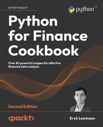
cerebro.plot(iplot=True, volume=False)Running the snippet generates the following plot:
Figure 12.6: Summary of our strategy’s behavior/performance over the backtested period
We can see that the strategy managed to make money, even after accounting for commission costs. The flat periods in the portfolio’s value represent periods when we did not have an open position.
- Investigate different returns metrics:
backtest_result[0].analyzers.returns.get_analysis()Running the code generates the following output:
OrderedDict([('rtot', 0.2365156915893157),
             ('ravg', 0.0009422935919893056),
             ('rnorm', 0.2680217199688534),
             ('rnorm100', 26.80217199688534)])
- Extract daily portfolio returns and plot them:
returns_dict = (
    backtest_result[0].analyzers.time_return.get_analysis()
)
returns_df = (
    pd.DataFrame(list(returns_dict.items()),
                 columns = ["date", "return"])
    .set_index("date")
)
returns_df.plot(title="Strategy's daily returns")

Figure 12.7: Daily portfolio returns of the strategy based on Bollinger bands
We can see that the flat periods in the portfolio’s returns in Figure 12.7 correspond to the periods during which we had no open positions, as can be seen in Figure 12.6.
How it works...
There are a lot of similarities between the code used for creating the Bollinger bands-based strategy and that used in the previous recipes. That is why we only discuss the novelties and refer you to the Event-driven backtesting with backtrader recipe for more details.
As we were going all-in in this strategy, we had to use a method called cheat_on_open. This means that we calculated the signals using day t’s close price, but calculated the number of shares we wanted to buy based on day t+1’s open price. To do so, we had to set cheat_on_open=True when instantiating the Cerebro object.
As a result, we also defined a next_open method instead of next within the Strategy class. This clearly indicated to Cerebro that we were cheating on open. Before creating a potential buy order, we manually calculated the maximum number of shares we could buy using the open price from day t+1.
When calculating the buy/sell signals based on the Bollinger bands, we used the CrossOver indicator. It returned the following:
- 1 if the first data (price) crossed the second data (indicator) upward
- -1 if the first data (price) crossed the second data (indicator) downward
We can also use CrossUp and CrossDown functions when we want to consider crossing from only one direction. The buy signal would look like this: self.buy_signal = bt.ind.CrossUp(self.datas[0], self.b_band.lines.bot).
The last addition included utilizing analyzers—backtrader objects that help to evaluate what is happening with the portfolio. In this recipe, we used two analyzers:
Returns: A collection of different logarithmic returns, calculated over the entire timeframe: total compound return, the average return over the entire period, and the annualized return.TimeReturn: A collection of returns over time (using a provided timeframe, in this case, daily data).
We can obtain the same result as from the TimeReturn analyzer by adding an observer with the same name: cerebro.addobserver(bt.observers.TimeReturn). The only difference is that the observer will be plotted on the main results plot, which is not always desired.
There’s more…
We have already seen how to extract the daily returns from the backtest. This creates a perfect opportunity to combine that information with the functionalities of the quantstats library. Using the following snippet, we can calculate a variety of metrics to evaluate our portfolio’s performance in detail. Additionally, we compare the performance of our strategy to a simple buy-and-hold strategy (which, for simplicity, does not include the transaction costs):
import quantstats as qs
qs.reports.metrics(returns_df,
                   benchmark="MSFT",
                   mode="basic")
Running the snippet generates the following report:
                    Strategy    Benchmark
------------------  ----------  -----------
Start Period        2021-01-04  2021-01-04
End Period          2021-12-30  2021-12-30
Risk-Free Rate      0.0%        0.0%
Time in Market      42.0%       100.0%
Cumulative Return   26.68%      57.18%
CAGR﹪              27.1%       58.17%
Sharpe              1.65        2.27
Sortino             2.68        3.63
Sortino/√2          1.9         2.57
Omega               1.52        1.52
For brevity’s sake, we only present the few main pieces of information available in the report.
In Chapter 11, Asset Allocation, we mentioned that an alternative library to quantstats is pyfolio. The latter has the potential disadvantage of not being actively maintained anymore. However, pyfolio is nicely integrated with backtrader. We can easily add a dedicated analyzer (bt.analyzers.PyFolio). For an example of implementation, please see the book’s GitHub repository.
Backtesting a moving average crossover strategy using crypto data
So far, we have created and backtested a few strategies on stocks. In this recipe, we cover another popular asset class—cryptocurrencies. There are a few key differences in handling crypto data:
- Cryptos can be traded 24/7
- Cryptos can be traded using fractional units
As we want our backtests to closely resemble real-life trading, we should account for those crypto-specific characteristics in our backtests. Fortunately, the backtrader framework is very flexible and we can slightly adjust our already-established approach to handle this new asset class.
Some brokers also allow for buying fractional shares of stocks.
In this recipe, we backtest a moving average crossover strategy with the following rules:
- We are only interested in Bitcoin and use daily data from 2021.
- We use two moving averages with window sizes of 20-days (fast one) and 50-days (slow one).
- If the fast MA crosses over the slow one upward, we allocate 70% of available cash to buying BTC.
- If the fast MA crosses over the slow one downward, we sell all the BTC we have.
- Short selling is not allowed.
How to do it…
Execute the following steps to implement and backtest a strategy based on the moving average crossover:
- Import the libraries:
import backtrader as bt import datetime import pandas as pd from backtrader_strategies.strategy_utils import * - Define the commission scheme allowing for fractional trades:
class FractionalTradesCommission(bt.CommissionInfo):
    def getsize(self, price, cash):
        """Returns the fractional size"""
        return self.p.leverage * (cash / price)
To make the code more readable, we first present the general outline of the class defining the trading strategy and then introduce the separate methods in the following substeps.
- Define the SMA crossover strategy:
class SMACrossoverStrategy(bt.Strategy): params = ( ("ma_fast", 20), ("ma_slow", 50), ("target_perc", 0.7) ) def __init__(self): # some code def log(self, txt): # some code def notify_order(self, order): # some code def notify_trade(self, trade): # some code def next(self): # some code def start(self): print(f"Initial Portfolio Value: {self.broker.get_value():.2f}") def stop(self): print(f"Final Portfolio Value: {self.broker.get_value():.2f}")- The
__init__method is defined as:def __init__(self): # keep track of close price in the series self.data_close = self.datas[0].close # keep track of pending orders self.order = None # calculate the SMAs and get the crossover signal self.fast_ma = bt.indicators.MovingAverageSimple( self.datas[0], period=self.params.ma_fast ) self.slow_ma = bt.indicators.MovingAverageSimple( self.datas[0], period=self.params.ma_slow ) self.ma_crossover = bt.indicators.CrossOver(self.fast_ma, self.slow_ma) - The
nextmethod is defined as:def next(self): if self.order: # pending order execution. Waiting in orderbook return if not self.position: if self.ma_crossover > 0: self.order = self.order_target_percent( target=self.params.target_perc ) log_str = get_action_log_string( "b", "c", price=self.data_close[0], size=self.order.size, cash=self.broker.getcash(), open=self.data_open[0], close=self.data_close[0] ) self.log(log_str) else: if self.ma_crossover < 0: # sell order log_str = get_action_log_string( "s", "c", self.data_close[0], self.position.size ) self.log(log_str) self.order = ( self.order_target_percent(target=0) )
- The
- Download the
BTC-USDdata:data = bt.feeds.YahooFinanceData( dataname="BTC-USD", fromdate=datetime.datetime(2020, 1, 1), todate=datetime.datetime(2021, 12, 31) ) - Set up the backtest:
cerebro = bt.Cerebro(stdstats=False) cerebro.addstrategy(SMACrossoverStrategy) cerebro.adddata(data) cerebro.broker.setcash(10000.0) cerebro.broker.addcommissioninfo( FractionalTradesCommission(commission=0.001) ) cerebro.addobserver(MyBuySell) cerebro.addobserver(bt.observers.Value) cerebro.addanalyzer( bt.analyzers.TimeReturn, _name="time_return" ) - Run the backtest:
backtest_result = cerebro.run()Running the snippet generates the following (abbreviated) log:
Initial Portfolio Value: 10000.00
2020-04-19: BUY CREATED - Price: 7189.42, Size: 0.97, Cash: 10000.00, Open: 7260.92, Close: 7189.42
2020-04-20: BUY EXECUTED - Price: 7186.87, Size: 0.97, Cost: 6997.52, Commission: 7.00
2020-06-29: SELL CREATED - Price: 9190.85, Size: 0.97
2020-06-30: SELL EXECUTED - Price: 9185.58, Size: -0.97, Cost: 6997.52, Commission: 8.94
2020-06-30: OPERATION RESULT - Gross: 1946.05, Net: 1930.11
…
Final Portfolio Value: 43547.99
In the excerpt from the full log, we can see that we are now operating with fractional positions. Also, the strategy has generated quite significant returns—we have approximately quadrupled the initial portfolio’s value.
- Plot the results:
cerebro.plot(iplot=True, volume=False)Running the snippet generates the following plot:

Figure 12.8: Summary of our strategy’s behavior/performance over the backtested period
We have already established that we have generated >300% returns using our strategy. However, we can also see in Figure 12.8 that the great performance might simply be due to the gigantic increase in BTC’s price over the considered period.
Using code identical to the code used in the previous recipe, we can compare the performance of our strategy to the simple buy-and-hold strategy. This way, we can verify how our active strategy performed compared to a static benchmark. We present the abbreviated performance comparison below, while the code can be found in the book’s GitHub repository.
                    Strategy    Benchmark
------------------  ----------  -----------
Start Period        2020-01-01  2020-01-01
End Period          2021-12-30  2021-12-30
Risk-Free Rate      0.0%        0.0%
Time in Market      57.0%       100.0%
Cumulative Return   335.48%     555.24%
CAGR﹪              108.89%     156.31%
Sharpe              1.6         1.35
Sortino             2.63        1.97
Sortino/√2          1.86        1.4
Omega               1.46        1.46
Unfortunately, our strategy did not outperform the benchmark over the analyzed timeframe. This confirms our initial suspicion that the good performance is connected to the increase in BTC’s price over the considered period.
How it works…
After importing the libraries, we defined a custom commission scheme in order to allow for fractional shares. Before, when we created a custom commission scheme, we inherited from bt.CommInfoBase and we modified the _getcommission method. This time, we inherited from bt.CommissionInfo and modified the getsize method to return a fractional value depending on the available cash and the asset’s price.
In Step 3 (and its substeps) we defined the moving average crossover strategy. By this recipe, most of the code will already look very familiar. A new thing we have applied here is the different type of order, that is, order_target_percent. Using this type of order indicates that we want the given asset to be X% of our portfolio.
It is a very convenient method because we leave the exact order size calculations to backtrader. If, at the moment of issuing the order, we are below the specified target percentage, we will buy more of the asset. If we are above it, we will sell some amount of the asset.
For exiting the position, we indicate that we want BTC to be 0% of our portfolio, which is equivalent to selling all we have. By using order_target_percent with the target of zero, we do not have to track/access the current number of units we possess.
In Step 4, we downloaded the daily BTC prices (in USD) from 2021. In the following steps, we set up the backtest, ran it, and plotted the results. The only thing worth mentioning is that we had to add the custom commission scheme (containing the fractional share logic) using the addcommissioninfo method.
There’s more…
In the recipe, we have introduced the target order. backtrader offers three types of target orders:
order_target_percent: Indicates the percentage of the current portfolio’s value we want to have in the given assetorder_target_size: Indicates the target number of units of a given asset we want to have in the portfolioorder_target_value: Indicates the asset’s target value in monetary units that we want to have in the portfolio
Target orders are very useful when we know the target percentage/value/size of a given asset, but do not want to spend additional time calculating whether we should buy additional units or sell them to arrive at the target.
There is also one more important thing to mention about fractional shares. In this recipe, we have defined a custom commission scheme that accounts for the fractional shares and then we used the target orders to buy/sell the asset. This way, when the engine was calculating the number of units to trade in order to arrive at the target, it knew it could use fractional values.
However, there is another way of using fractional shares without defining a custom commission scheme. We simply need to manually calculate the number of shares we want to buy/sell and create an order with a given stake. We did something very similar in the previous recipe, but there, we rounded the potential fractional values to an integer. For an implementation of the SMA crossover strategy with manual fractional order size calculations, please refer to the book’s GitHub repository.
Backtesting a mean-variance portfolio optimization
In the previous chapter, we covered asset allocation and mean-variance optimization. Combining mean-variance optimization with a backtest would be an interesting exercise, especially because it involves working with multiple assets at once.
In this recipe, we backtest the following allocation strategy:
- We consider the FAANG stocks.
- Every Friday after the market closes, we find the tangency portfolio (maximizing the Sharpe ratio). Then, we create target orders to match the calculated optimal weights on Monday when the market opens.
- We assume we need to have at least 252 data points to calculate the expected returns and the covariance matrix (using the Ledoit-Wolf approach).
For this exercise, we download the prices of the FAANG stocks from 2020 to 2021. Due to the warm-up period we set up for calculating the weights, the trading actually happens only in 2021.
Getting ready
As we will be working with fractional shares in this recipe, we need to use the custom commission scheme (FractionalTradesCommission) defined in the previous recipe.
How to do it…
Execute the following steps to implement and backtest a strategy based on the mean-variance portfolio optimization:
- Import the libraries:
from datetime import datetime
import backtrader as bt
import pandas as pd
from pypfopt.expected_returns import mean_historical_return
from pypfopt.risk_models import CovarianceShrinkage
from pypfopt.efficient_frontier import EfficientFrontier
from backtrader_strategies.strategy_utils import *
To make the code more readable, we first present the general outline of the class defining the trading strategy and then introduce the separate methods in the following substeps.
- Define the strategy:
class MeanVariancePortfStrategy(bt.Strategy): params = (("n_periods", 252), ) def __init__(self): # track number of days self.day_counter = 0 def log(self, txt): dt = self.datas[0].datetime.date(0).isoformat() print(f"{dt}: {txt}") def notify_order(self, order): # some code def notify_trade(self, trade): # some code def next(self): # some code def start(self): print(f"Initial Portfolio Value: {self.broker.get_value():.2f}") def stop(self): print(f"Final Portfolio Value: {self.broker.get_value():.2f}")- The
nextmethod is defined as:def next(self): # check if we have enough data points self.day_counter += 1 if self.day_counter < self.p.n_periods: return # check if the date is a Friday today = self.datas[0].datetime.date() if today.weekday() != 4: return # find and print the current allocation current_portf = {} for data in self.datas: current_portf[data._name] = ( self.positions[data].size * data.close[0] ) portf_df = pd.DataFrame(current_portf, index=[0]) print(f"Current allocation as of {today}") print(portf_df / portf_df.sum(axis=1).squeeze()) # extract the past price data for each asset price_dict = {} for data in self.datas: price_dict[data._name] = ( data.close.get(0, self.p.n_periods+1) ) prices_df = pd.DataFrame(price_dict) # find the optimal portfolio weights mu = mean_historical_return(prices_df) S = CovarianceShrinkage(prices_df).ledoit_wolf() ef = EfficientFrontier(mu, S) weights = ef.max_sharpe(risk_free_rate=0) print(f"Optimal allocation identified on {today}") print(pd.DataFrame(ef.clean_weights(), index=[0])) # create orders for allocation in list(ef.clean_weights().items()): self.order_target_percent(data=allocation[0], target=allocation[1])
- The
- Download the prices of the FAANG stocks and store the data feeds in a list:
TICKERS = ["META", "AMZN", "AAPL", "NFLX", "GOOG"] data_list = [] for ticker in TICKERS: data = bt.feeds.YahooFinanceData( dataname=ticker, fromdate=datetime(2020, 1, 1), todate=datetime(2021, 12, 31) ) data_list.append(data) - Set up the backtest:
cerebro = bt.Cerebro(stdstats=False) cerebro.addstrategy(MeanVariancePortfStrategy) for ind, ticker in enumerate(TICKERS): cerebro.adddata(data_list[ind], name=ticker) cerebro.broker.setcash(1000.0) cerebro.broker.addcommissioninfo( FractionalTradesCommission(commission=0) ) cerebro.addobserver(MyBuySell) cerebro.addobserver(bt.observers.Value) - Run the backtest:
backtest_result = cerebro.run()
Running the backtest generates the following log:
Initial Portfolio Value: 1000.00
Current allocation as of 2021-01-08
  META  AMZN  AAPL  NFLX  GOOG
0 NaN   NaN   NaN   NaN   NaN
Optimal allocation identified on 2021-01-08
  META     AMZN     AAPL  NFLX  GOOG
0  0.0  0.69394  0.30606   0.0   0.0
2021-01-11: Order Failed: AAPL
2021-01-11: BUY EXECUTED - Price: 157.40, Size: 4.36, Asset: AMZN, Cost: 686.40, Commission: 0.00
Current allocation as of 2021-01-15
  META  AMZN  AAPL  NFLX  GOOG
0  0.0   1.0   0.0   0.0   0.0
Optimal allocation identified on 2021-01-15
  META     AMZN     AAPL  NFLX  GOOG
0  0.0  0.81862  0.18138   0.0   0.0
2021-01-19: BUY EXECUTED - Price: 155.35, Size: 0.86, Asset: AMZN, Cost: 134.08, Commission: 0.00
2021-01-19: Order Failed: AAPL
Current allocation as of 2021-01-22
  META  AMZN  AAPL  NFLX  GOOG
0  0.0   1.0   0.0   0.0   0.0
Optimal allocation identified on 2021-01-22
  META     AMZN     AAPL  NFLX  GOOG
0  0.0  0.75501  0.24499   0.0   0.0
2021-01-25: SELL EXECUTED - Price: 166.43, Size: -0.46, Asset: AMZN, Cost: 71.68, Commission: 0.00
2021-01-25: Order Failed: AAPL
...
0  0.0   0.0  0.00943   0.0  0.99057
2021-12-20: Order Failed: GOOG
2021-12-20: SELL EXECUTED - Price: 167.82, Size: -0.68, Asset: AAPL, Cost: 110.92, Commission: 0.00
Final Portfolio Value: 1287.22
We will not spend time evaluating the strategy, as this would be very similar to what we did in the previous recipe. Thus, we leave it as a potential exercise for the reader. It could also be interesting to test the performance of this strategy against a benchmark 1/n portfolio.
It is worth mentioning that some of the orders failed. We will describe the reason for it in the following section.
How it works…
After importing the libraries, we defined the strategy using mean-variance optimization. In the __init__ method, we defined a counter that we used to determine if we had enough data points to run the optimization routine. The selected 252 days is arbitrary and you can experiment with different values.
In the next method, there are multiple new components:
- We first add 1 to the day counter and check if we have enough observations. If not, we simply proceed to the next trading day.
- We extract the current date from the price data and check if it is a Friday. If not, we proceed to the next trading day.
- We calculate the current allocation by accessing the position size of each asset and multiplying it by the close price of the given day. Lastly, we divide each asset’s worth by the total portfolio’s value and print the weights.
- We need to extract the last 252 data points for each stock for our optimization routine. The
self.datasobject is an iterable containing all the data feeds we pass toCerebrowhen setting up the backtest. We create a dictionary and populate it with arrays containing the 252 data points. We extract those using thegetmethod. Then, we create apandasDataFrame from the dictionary containing the prices. - We find the weights maximizing the Sharpe ratio using the
pypfoptlibrary. Please refer to the previous chapter for more details. We also print the new weights. - For each of the assets, we place a target order (using the
order_target_percentmethod) with the target being the optimal portfolio weight. As we are working with multiple assets this time, we need to indicate for which asset we are placing an order. We do so by specifying thedataargument.
Under the hood, backtrader uses the array module for storing the matrix-like objects.
In Step 3, we created a list containing all the data feeds. We simply iterated over the tickers of the FAANG stocks, downloaded the data for each one of them, and appended the object to the list.
In Step 4, we set up the backtest. A lot of the steps are already very familiar by now, including setting up the fractional shares commission scheme. The new component was adding the data, as we iteratively added each of the downloaded data feeds using the already covered adddata method. At this point, we also had to provide the name of the data feeds using the name argument.
In the very last step, we ran the backtest. As we have mentioned before, the new thing we can observe here is the failing orders. These are caused by the fact that we are calculating the portfolio weights on Friday using the close prices and preparing the orders on the same day. On Monday’s market open, the prices are different, and not all the orders can be executed. We tried to account for that using fractional shares and setting the commission to 0, but the differences can still be too big for this simple approach to work. A possible solution would be to always keep some cash on the side to cover the potential price differences.
To do so, we could assume that we purchase the stocks with ~90% of our portfolio’s worth while keeping the rest in cash. For that, we could use the order_target_value method. We could calculate the target value for each asset using the portfolio weights and 90% of the monetary value of our portfolio. Alternatively, we could use the DiscreteAllocation approach of pypfopt, which we mentioned in the previous chapter.
Summary
In this chapter, we have extensively covered the topic of backtesting. We started with the simpler approach, that is, vectorized backtesting. While it is not as rigorous and robust as the event-driven approach, it is often faster to implement and execute, due to its vectorized nature. Afterward, we combined the exploration of the event-driven backtesting framework with the knowledge we obtained in the previous chapters, for example, calculating various technical indicators and finding the optimal portfolio weights.
We spent the most time using the backtrader library, due to its popularity and flexibility when it comes to implementing various scenarios. However, there are many alternative backtesting libraries on the market. You might also want to investigate the following:
vectorbt(https://github.com/polakowo/vectorbt): Apandas-based library for efficient backtesting of trading strategies at scale. The author of the library also offers a pro (paid) version of the library with more features and improved performance.bt(https://github.com/pmorissette/bt): A library offering a framework based on reusable and flexible blocks containing the strategy’s logic. It supports multiple instruments and outputs detailed statistics and charts.backtesting.py(https://github.com/kernc/backtesting.py): A backtesting framework built on top ofbacktrader.fastquant(https://github.com/enzoampil/fastquant): A wrapper library aroundbacktraderthat aims to reduce the amount of boilerplate code we need to write in order to run a backtest for popular trading strategies, for example, the moving average crossover.zipline(https://github.com/quantopian/zipline / https://github.com/stefan-jansen/zipline-reloaded): The library used to be the most popular (based on GitHub stars) and probably the most complex of the open-source backtesting libraries. However, as we have already mentioned, Quantopian was closed and the library is not maintained anymore. You can use the fork (zipline-reloaded) maintained by Stefan Jansen.
Backtesting is a fascinating field and there is much more to learn about it. Below, you can also find some very interesting references for more robust approaches to backtesting:
- Bailey, D. H., Borwein, J., Lopez de Prado, M., & Zhu, Q. J. (2016). “The probability of backtest overfitting.” Journal of Computational Finance, forthcoming.
- Bailey, D. H., & De Prado, M. L. (2014). “The deflated Sharpe ratio: correcting for selection bias, backtest overfitting, and non-normality.” The Journal of Portfolio Management, 40 (5), 94-107.
- Bailey, D. H., Borwein, J., Lopez de Prado, M., & Zhu, Q. J. (2014). “Pseudo-mathematics and financial charlatanism: The effects of backtest overfitting on out-of-sample performance.” Notices of the American Mathematical Society, 61 (5), 458-471.
- De Prado, M. L. (2018). Advances in Financial Machine Learning. John Wiley & Sons.