14.2.1 The Mandelbrot Set

“The Mandelbrot set is the set of complex numbers c having magnitude ≤ 2 for which the function f_c(z) = z² + c does not diverge when iterated from z = 0, i.e., for which the sequence f_c(0), f_c(f_c(0)), etc., remains bounded in absolute value.”¹ In other words, if we pick a random complex number c with magnitude ≤ 2 and initialize the complex number z to zero, at what iteration i will the recurrence exceed magnitude 2? The set is often visualized as a contour plot of iteration count, i, as a function of the real and imaginary components of z.

While a “toy” problem, several aspects make computing terms of the Mandelbrot set useful in illustrating HPC problems: the algorithm is easy to describe, can be implemented with little code, can be vectorized and readily implemented in parallel yet has nontrivial load balancing aspects, and can be made arbitrarily large. The fascinating images that arise are a nice side benefit.

14.2.2 A 2D Finite Element Solver

Many excellent finite element (FE) packages are available for Python. Industrial-strength applications include deal.II², FEniCS³, SfePy⁴, and Code-Aster.⁵ These are substantial projects with hundreds of thousands of lines of source code developed by many domain experts.

The K produced in step 3 is exceptionally sparse; a typical mesh of rod elements derived from triangle’s output leaves on average of just 14 non-zero terms per row or column. M is a diagonal matrix. As a result, a million degree of freedom models can be processed quite easily with 8 GB of memory. The names of the Python and MATLAB finite element source files appear in Appendix C; the source files themselves are available on the book's Github repository.⁶

The mesh from beam.2.ele and beam.2.node, for example, looks like this:

The last pair of files, beam.5.ele and beam.5.node, are 32 MB and 28 MB and define a mesh with more than a million degrees of freedom.

14.4.1 Mandelbrot Set Performance

MATLAB does well on this problem as it runs three times faster than the Python version. Table 14-1 shows elapsed times for a variety of N × N image sizes.

The larger values of N may seem excessive, but their inclusion will be apparent once we begin applying optimization techniques.

14.4.2 FE Solver Performance

The third stage combines floating-point computations for element matrix generation and sparse matrix creation. The final stage, computing the smallest six eigenvalues and corresponding eigenvectors of the sparse matrices, is dominated by floating-point computation.

Python code outperforms MATLAB on the first three stages—and the total solution time—but MATLAB’s eigensolution is notably faster. Reading model data from text files in particular is ten times faster in Python than MATLAB. Python also uses considerably less memory than MATLAB.

14.5.1 Scalene

Scalene [1] is a low overhead sampling profiler that additionally reports GPU use (if a GPU is detected), memory copy metrics, and memory consumption—all at a per-line level.

Scalene is unique among Python code profilers for several reasons. Its primary killer feature is stratifying CPU results on each line to time spent in pure Python, time spent in underlying compiled libraries (referred to as “native” time), and system time (for I/O and operations not related to the code). This separation helps answer the implied question of what to do about a slow line of code. If the bulk of time is in pure Python, there might be a way to rewrite the code to call a faster library function. On the other hand, if most of the time is taken by an underlying library or the system, there may be less opportunity for improvement. Scalene also works with multiple threads and processes.

Lines 8 and 9 are shown to be the hot spots, consuming nearly 90% of the solution time. The memory results on the other hand are counterintuitive because peak use is shown to happen on a line that simply multiplies and adds complex scalars.

The portion of profile.html showing the single most expensive line of code—12% overall CPU time spent returning an element stiffness matrix—looks like this in a browser:

Interestingly, the scalene results suggest the time was spent copying memory rather than performing computations.

14.5.2 Austin and FlameGraph

Austin ⁸ is another sampling profiler. Like scalene, it adds little overhead, requires no change to the code being profiled, and can send results to other metrics tools such as FlameGraph⁹ for graphical display. (MATLAB’s profiler also displays timing results as FlameGraphs, although with a slate gray color scheme instead of red/orange/yellow.)

FlameGraphs represent the call stack vertically, with the main program at the bottom. The width of each bar represents the amount of time spent at a particular function in MATLAB or line of code with austin; hot spots in the code appear as the widest bars. The left-to-right arrangement of bars is arbitrary and does not indicate chronological execution sequence. Bar colors also are arbitrary. Vertical arrangement is significant: code represented by a bar calls the code in the bars immediately above it. The lowest bar is, naturally, the widest as it represents the program’s main function entry point. Recognizable function names generally appear at the third or fourth bars from the bottom.

The --minwidth 10 switch to FlameGraph excludes entries that would leave a bar fewer than 10 pixels wide. Without it, the graph would be cluttered with entries having inconsequential contributions that make it harder to interpret. Raise or lower this pixel width value to produce the level of resolution that interests you. FlameGraph’s output is an SVG file which can be viewed with a web browser. The image

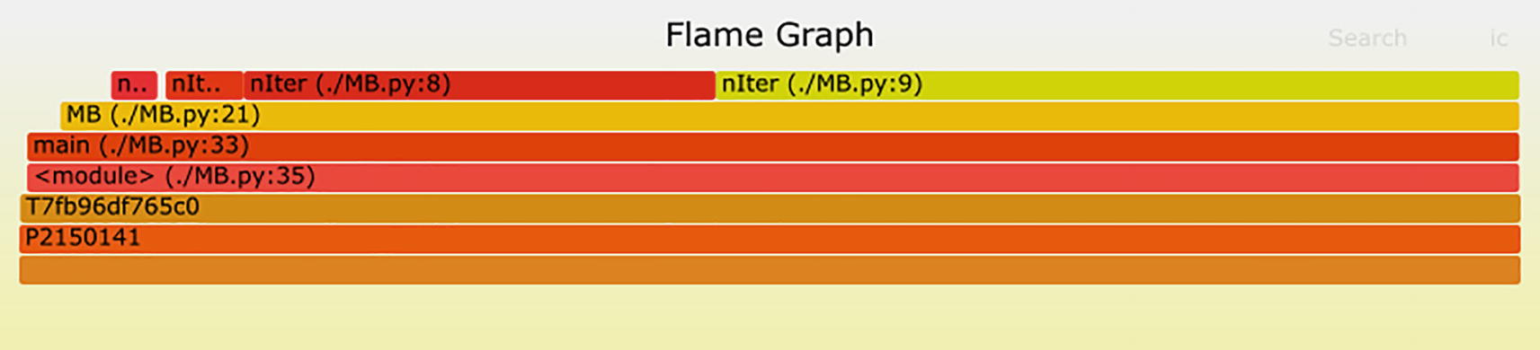
shows the bulk of compute time is spent in function nIter() at lines 8 and 9. Recall from Section 14.2.1 that nIter()’s implementation is

The computational effort at lines 8 and 9 happens with the statements z = z*z + c and if abs(z) > 2.

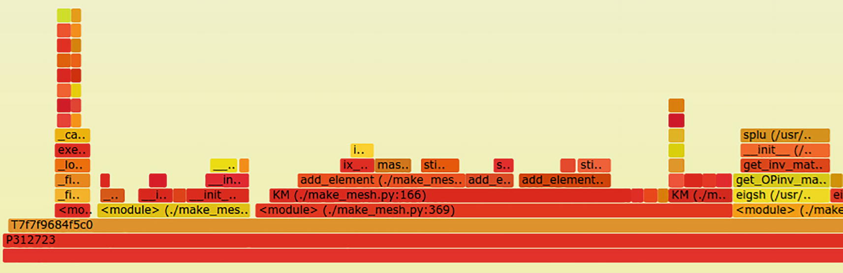
The same profiling command run against the finite element solver for the beam.4 case produces a more complex plot.

14.8.1 Python Compiled with Cython

A setup file that works for the third step looks like this:

A typical invocation produces warnings, then new C source files, and, hopefully, a shared object named after the .pyx file. On my Linux machine, the shared object is MB_cython.cpython-38-x86_64-linux-gnu.so. Despite the long name, it is imported into Python with import MB_cython.

What have we gained for our efforts? A small driver program loads the compiled module and runs the cases:

For N = 1000, runtime drops from 17.1 seconds to just 1.85 seconds. The original Python code is 3x slower than MATLAB, but Cython enhancements have made Python 3x faster.

This single line refinement cuts the N = 1000 Python+Cython time from 1.85 to 1.01 seconds, and the MATLAB time, with an equivalent change, from 5.8 to 4.4 seconds.

14.8.2 Parallel for Loops with Cython

The core MATLAB product does not include the parfor parallel for loop command—that can only be found in MATLAB Coder or the Parallel Computing Toolbox. MATLAB implementations in this book are therefore limited to sequential for loops.

Cython has a prange() function that allows one to write parallel for loops. Under the hood, this prange() function is implemented via OpenMP and therefore inherits OpenMP restrictions. The Cython documentation shows trivial parallel for loop examples,¹¹ but in practice, nontrivial loops require an inordinate amount of code tweaks to overcome compile error such as “Indexing Python object not allowed without gil,” “Constructing Python tuple not allowed without gil,” and “Coercion from Python not allowed without the GIL.”

Unless your code sections have elementary for loops, you will either need to spend a lot of time with the Cython documentation or avoid its prange(). The Pythran and Numba options for parallel for loops, described in Sections 14.9 and 14.10.1, are much easier to use.

14.8.3 Cython Performance

14.9.1 Examples of Signature Comments

The comment line preceding the definition of a function Fn() which takes a string, a list of integers, and a 2D array of 32-bit floats would therefore be

14.9.2 Python Compiled with Pythran; Parallel for Loops

As with Cython, the Mandelbrot functions nIter() and MB() are separated to their own file for compilation. Only three comment lines are needed to enable Pythran to compile our code:

The first two comments define signatures (excluding return type, which Pythran figures out on its own) of the functions on the following lines, and the third comment designates the for i,I loop to be parallel.

Among other things, Pythran needs the C header file to the basic linear algebra subroutines (BLAS). If your compile command shows

and does not create a shared object file, you’ll need to download and install development headers for BLAS suitable to your OS. On Ubuntu, for example, this is resolved with apt install libopenblas-dev. Even after installing the headers, you may still see the “fatal error” even though the shared object file is created successfully.

To suppress OpenMP parallelism of the for loop, either remove the #omp parallel for comment from the source or remove the -fopenmp switch from the compile command.

The pythran command produces a compiled shared object file named after the input source file (MB_pythran.cpython-38-x86_64-linux-gnu.so on my computer). The driver program to run the Pythran-compiled module is identical to the driver used for the Cython-compiled module. The only difference is the name of the module being loaded—import MB_pythran instead of import MB_cython:

14.9.3 Pythran Performance

14.10.1 Parallel for Loops with Numba

Numba’s prange() function resembles Cython’s. Writing a parallel for loop amounts to replacing the existing for i in ... construct with for i in prange(N) where N is an integer scalar. The requirement that the loop iterate over a range of integers may mean the loop needs small modifications if the existing loop iterates over other objects.

Numba handles the distribution of work in the body of the loop to different cores as well as aggregation of results for variables shared between simultaneous computations.

14.10.2 Numba Keyword Arguments nopython, fastmath

The @jit() keyword argument nopython, most often seen set to True, instructs the JIT compiler to skip the Python interpreter completely and use only compiled code. This is the recommended setting and even has its dedicated decorator: @njit() is the same as @jit(...,nopython=True). This keyword should only be set to False if the compilation fails.

The keyword argument fastmath enables unsafe operations¹⁴ such as assuming inputs are never NaNs or Infs and allows the compiler to reorder floating-point instructions. Naturally, compare output of your code with and without fastmath=True to ensure your results are not compromised.

14.10.3 Numba Performance

Performance of the Numba-enhanced Mandelbrot program, shown in Table 14-8, is nothing less than astonishing. With Numba, pure Python code exceeds the speed of Cython- and Pythran-compiled modules.

14.10.4 Numba Limitations

Unless one employs Numba’s Wrapper Address Protocol,¹⁵ functions decorated by @jit may call only a subset of NumPy and standard library functions.

and a call to XYZ() exists in a function decorated by @jit, it means Numba cannot compile this function. In this case, your options are to simplify the function until it can be compiled, revert to the multiprocessing module (Section 14.6), or use dask, to be covered in Section 14.13.

14.12.1 Compile Python Modules in a MATLAB-Friendly Virtual Environment

Three of the next four sections, Sections 14.12.2, 14.12.3, and 14.12.5, use your computer’s C, C++, or Fortran compiler to build binary Python modules. On macOS, this means the Xcode development library must be installed. On all operating systems, it is important to work in a conda environment like matpy (Section 2.​5.​1) whose shared libraries are consistent with MATLAB’s. The compiled modules won’t load in MATLAB otherwise.

14.12.2 MATLAB + Cython

This driver loads the MB_cython module compiled in Section 14.11.

14.12.3 MATLAB + Pythran

This driver loads the MB_pythran module compiled in Section 14.9.

14.12.4 MATLAB + Numba

This driver loads the parallel for loop MB_numba_prange module of Section 14.10.

14.12.5 MATLAB + f2py

This driver loads the MB_fortran module compiled in Section 14.11.

14.12.6 MATLAB + Python Performance Results

While the single-core f2py performance is modest compared to multicore Numba performance, f2py offers a secondary benefit the other accelerants lack: with f2py you can create a Fortran interface to MATLAB much more easily than you can with MATLAB’s own mex utility.

14.13.1 Parallel MATLAB

Like Python, MATLAB can run on distributed memory clusters and on clusters in the cloud. The most direct way to do so is to use the Parallel Computing Toolbox. Other options include using MATLAB Coder or the MATLAB Compiler to create a stand-alone executable that can be sent to remote computers.

The MathWorks also offers MATLAB Online, and through it, MATLAB in the Cloud, but its capabilities are limited to those enabled in your MATLAB license. In other words, if you don’t have a license for the Parallel Computing Toolbox or for cloud use, you won’t be able to run your m-files on multiple computers in the cloud.

As mentioned earlier (Section 1.​3), this book’s scope is limited to the core MATLAB product which precludes comparisons of pure MATLAB cloud solutions to their Python equivalents. Nonetheless, we’ll see in Section 14.14 that hybrid MATLAB/Python code runs quite effectively on private clusters as well as Coiled’s cloud.

14.13.2 Dask Execution Paradigm and Performance Expectations

A dask-enabled Python program populates a list with delayed tasks and then passes this list to dask.compute(). This function hands tasks off to the dask scheduler which in turn sends each task to the next idle worker (likely running on a different computer). After a worker receives a task, the worker calls the user-provided function defined for the task with the user’s arguments, then sends its return values back to the scheduler. dask.compute() gets the task return values from the scheduler and appends these to its list of results.

Our program sets up the function calls to be made in parallel, and dask handles everything else—assigning these calls to processors, serializing and then sending input arguments over the network, invoking the calls on remote computers, and finally serializing and sending the return arguments back to the computer which launched the jobs.

Most importantly, dask decides how and when to transmit data. Code developers are generally happy to offload this burden even if the interleaving of compute/transmit steps isn’t ideal, yet may be disappointed by the ensuing parallel efficiency. The adage “your mileage may vary” is ever true in parallel processing.

This all sounds complicated (and under the hood, it is!). How exactly do we set up and run a distributed memory parallel program? What can be done to make the code run faster? The only way to make sense of this is to work through examples.

14.13.3 Example 1: Sum of Prime Factors on One Computer

Calls to the compute-intensive function my_fn() are independent and can be called in any order, or even simultaneously. We’ll do exactly that with dask, using three cores of the local machine. To spread the load evenly, we merely need to offset the starting counter by the job number and let the call to range(a,b,incr) in my fn() scatter the numbers to factor across processors. For example, if we compute prime factors for numbers between 2 and 20 and want to spread the work evenly over three jobs, the assignments will be

or equivalently in MATLAB

The dask-enabled version of the prime factor summation program on the local computer, splitting up the work to three tasks that are to run simultaneously, looks like this:

When the program runs, the call to Client(’127.0.0.1:8786’) at line 16 attempts to connect to a dask scheduler running on the localhost and listening on port 8786. (Line 17, currently commented out, will be discussed in Section 14.13.5.) If such a scheduler isn’t running, the program fails after 30 seconds with

Line 21 defines n_jobs, our counter for the number of tasks to create. At a minimum, to take full advantage of your hardware, this should equal or exceed the number of cores available in your cluster. If tasks vary in duration and you have many of them, setting n_jobs to a value much greater than the number of cores will help balance the load across cores more equitably.

Lines 24–26 add delayed tasks to the list tasks which was initialized at line 18. Each task is a call to my_fn() with arguments A+i, B, incr.

The computations are performed at line 27 when dask hands the list of delayed tasks to the scheduler to farm out to workers. Return values from each call appear in the list results which will have n_jobs entries.

Finally, lines 29–32 aggregate the partial sums of primes into a total value.

then passing this file name as an argument to the dask-ssh command:

This starts a worker process on each computer defined in the file, plus a scheduler process on the computer defined on the first line. Of course, in this case, all these background processes run on the local computer.

With the scheduler and workers running in the background, we can now run the dask-enabled prime factor summation program prime_dask.py. It runs faster than the sequential version, but not by much:

Performance disappoints for two reasons. First, the workload is clearly imbalanced since one job took around 200 seconds, while the other two took more than 320. Evidently, terms of the sequence 3, 6, 9 … can be factored much more rapidly than terms in 2, 5, 8 … and 4, 7, 10 …—who knew? The second reason is less obvious. It is that the sum of individual core times, 328.0 + 206.2 + 327.7 = 861.9 seconds, is 66% higher than the single-core time of 519.5 seconds. Dask seems to impose a severe overhead.

Three experiments shed light on the source of dask’s overhead. First, we’ll repeat the single-core runtime using the dask infrastructure with only one worker process, meaning only one CPU core will receive work. A scheduler is always needed so that must also run in the background. Performance in this case is reasonable since dask added less than 7% overhead (555.0 seconds vs. 519.5 seconds):

Next, we’ll spin up two more dask worker processes, but still only submit one job:

This time, overhead doubled to 13% even though the additional two workers are merely standing by, waiting for work that never comes.

Finally, we’ll again use just one worker but give it three tasks where the ranges are separated by strides of three, just as when these ranges are given to three workers.

The cause of the overhead must be related to how the work is split up. While there’s no obvious remedy to improve this situation, dask does have nice performance monitoring and reporting tools to help diagnose performance issues. One of these tools is the web-based real-time cluster statistics seen on the scheduler host’s port 8787, http://127.0.0.1:8787 in our case. Another is a report generator that can be invoked directly from our program. We merely need to import the performance_report function from dask.distributed and then wrap the dask-specific code in a context manager that calls performance_report to get a rich HTML file graphically showing many different aspects of the parallel job.

While the reporting tool is easy to use, comprehending the output is less so.

14.13.4 Setting Up a Dask Cluster on Multiple Computers

Running dask on a single computer is a useful first step during code development and initial troubleshooting. It fails to satisfy on the performance front, however. To really benefit from dask’s power, we’ll need to run it on many computers.

14.13.5 Example 2: Sum of Prime Factors on Multiple Computers

Once the computers in the dask cluster are running a scheduler and workers, we can begin to enjoy significant performance increases. This section uses a collection of 18 virtual machines running on DigitalOcean’s²² cloud infrastructure. Each VM runs their lowest tier “droplet” which has 1 GB of memory, 1 CPU core @ 2.5 GHz, and 25 GB of storage. The VMs run Ubuntu 20.04.3 LTS, have Anaconda 2021.05 installed, and use the matpy conda environment (Section 2.​5.​1).

where DigitalOcean_VMs.txt has the IP addresses of all 18 computers. The only change needed to prime_dask.py (code listing in Section 14.13.3) is replacing the call to Client(127.0.0.1:8786) with the IP address of the VM running the scheduler, in other words, the first entry in DigitalOcean_VMs.txt. Line 17 shows what this might look like.

The sequential version of the program takes 718.057 seconds on a single VM, so the 18 cores gave a 16.5 × speed-up.

14.13.6 Example 3: A Gigapixel Mandelbrot Image

In Section 14.10.3, we used Numba to reduce the time needed to compute a 5000 x 5000 Mandelbrot image from 420 seconds to about 9 seconds on one core. Let’s up the stakes and use our dask cluster of 18 single-core VMs to compute an image with 35,000 x 35,000—1.2 billion—pixels. Each pixel will be represented by a single byte which is the number of iterations needed for the z equation to converge. Both MATLAB and Python running on a computer with at least 8 GB of memory can easily store such an image; MATLAB can even display it with imshow() (matplotlib’s imshow() crashes with an image this size).

Our gigapixel image will be 7², or about 50x larger than our 5k image so a single Numba-powered core should take about 440 seconds to generate it. Then, again, our dask cluster has 18 computers, so if we can load balance the jobs well, that time will come down by a lot. Let’s give it a shot.

One strategy for load balancing the Mandelbrot set is to assign rows or columns to workers in a round-robin fashion. Here’s what the dask + Numba solution looks like with that strategy:

In other words, the workers crashed because they ran out of memory. While the computer submitting the job has 8 GB of memory, the workers only have 1 GB, some of which is taken by the operating system and the dask worker processes.

Rather than have each remote computer accumulate all results for the jobs it was assigned, we’ll need to harvest results from the remote computers as the run progresses. One way to do that is to split the jobs into groups and then call the .compute() method after each group is submitted. The revised version of the following Mandelbrot program does just that. An additional modification is implemented to improve parallel efficiency: instead of sending the real and imaginary arrays to the remote workers, we’ll just send the starting and ending values and let the workers figure out the array terms on their own. Finally, to simplify reassembly of the final image, we’ll have each worker tell us the row indices it worked on in addition to its image slices.

My original estimate for solving the Numba-accelerated Mandelbrot set of this size on a single core of my home computer was 440 seconds, so the 83 seconds using 18 cloud-based computers represents a speed-up of 5.3. Disappointing, perhaps, but a clear demonstration that performance for problems involving substantial data transfers depends heavily on the network.

14.13.7 Example 4: Finite Element Frequency Domain Response

As in the multicore sections earlier, I’ll use a finite element model subject to a dynamic load to represent a more real-world distributed memory computing problem. Toy problems for summing prime numbers and computing the Mandelbrot set are instructional but don’t deal with complications that arise with large input sets.

Simulating the behavior of structures subject to a sudden acceleration, for example, an impact, or the firing of explosive bolts (common in spacecraft that release articulating members) is tricky. A finite element model suited to such work needs small elements to capture the short wavelengths of the resulting structural waves. The spectral content of impacts and explosions is high, so if a modal analysis were undertaken, many eigensolutions—often an impractical number—would be needed. Alternatively, one could attempt a direct time integration (e.g., with the Newmark-beta method) of the equilibrium equation of motion:

u(t) and P(t) are the time-varying response and applied load. A third possibility is where M, C, and K are finite element mass, damping, and stiffness matrices, and perfect for large parallel computers: transform the equilibrium equation to the frequency domain where each of the many frequencies can be worked on independently. Such a transformation can be done with the substitution:

which leaves a series of N linear equations

Or

where P(ω) is the Fourier transform of the load time history P(t). Our time domain second-order differential equation now becomes a collection of linear equations which are independent at each of the N frequencies ω_n. The frequency band must be sufficiently wide to capture the full spectral content of the applied load, and the frequency interval small enough that all motion has been dampened to a quiescent state in the equivalent time domain.

In theory, if we had N processors, we could give each processor one frequency and get our solution in the amount of time it takes to solve the system of equations just once. The time domain solution u(t) can then be recovered with an inverse Fourier transform of [2]. In reality, thousands of frequencies are needed for accurate solutions, and a few of us have access to that many processors. Also, the data volumes are substantial; the overhead of transmitting matrices to a processor so it can solve a system of linear equations just once is unlikely to be worthwhile.

For our final example, we’ll use dask to solve a direct frequency response problem. This example is more representative of real workloads because, unlike the earlier problems, this one requires large amounts of input data to be sent to the workers.

14.13.7.1 A Notional Satellite Model

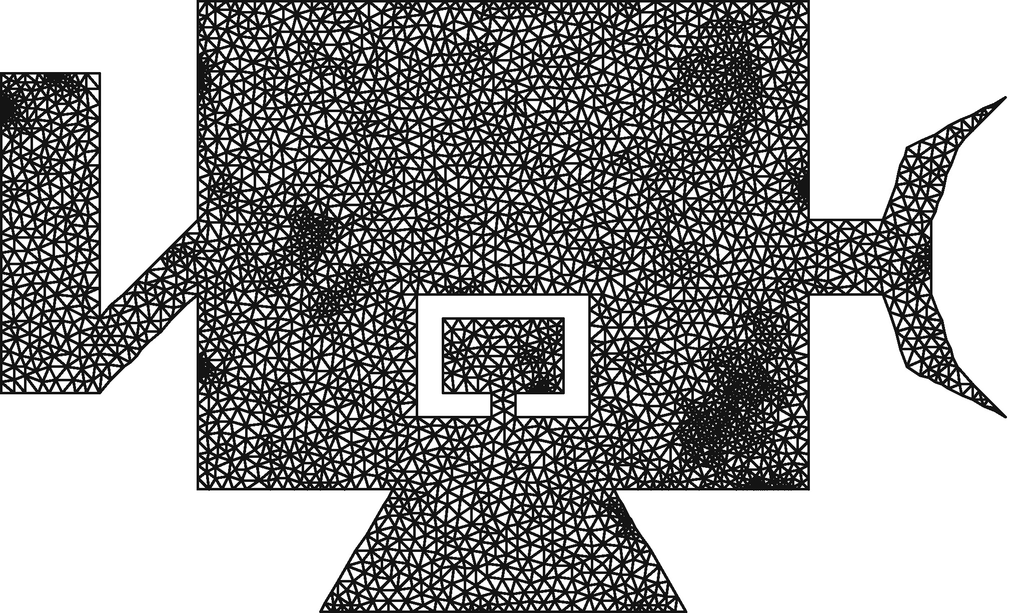
As a sample problem, we’ll model a satellite whose solar panel extension mechanism is to be released by an explosive bolt. The satellite has a delicate sensor in the middle. Our objective is to measure the deformation of the sensor’s mount as a result of the detonation.

Once again, we’ll use triangle to tessellate a boundary file, satellite/satellite.poly, to a series of increasingly finer finite element meshes:

triangle -pa0.8        satellite.poly

triangle -rpq34a0.2    satellite.1

triangle -rpq34a0.1    satellite.2

triangle -rpq34a0.05   satellite.3

triangle -rpq34a0.02   satellite.4

triangle -rpq34a0.015  satellite.5

triangle -rpq34a0.005  satellite.6

After the last command, we’ll have a pair of files satellite.7.ele and satellite.7.node, that define a model with about 600,000 degrees of freedom that we’ll use for the analysis. The model will be fully constrained at the base of the adapter ring (the lowest horizontal edge) and loaded (meaning the location of the explosive bolt) at the elbow joint on the left. We’ll only save deformation at the few nodes that represent the sensor’s mount which is the small stem supporting the central cutout. The following figure is of the second refinement of the model, satellite.2, which has about 7600 degrees of freedom (roughly 1% of our 600k DOF model).

Time and frequency domain plots of the explosive bolt’s load history look like this:

14.13.7.3 Sending Large Inputs to Remote Computers

Our solution strategy will be to send each remote computer a subset of frequencies, ω_n; the three finite element matrices K, C, and M; load vector b; the load spectrum ; and the list of degrees of freedom at which we want the response. Unlike the examples for prime number summation and Mandelbrot set, for this problem we have to send huge arrays totalling hundreds of megabytes or more to each worker. (A .mat file of K, C, M, and b for satellite.7 is 224 MB.) Fortunately, dask has a data distribution mechanism—a client’s .scatter() method followed by a client _submit()—to handle this situation. The following code fragments show the conventional method to send data to remote workers on the left and the data distribution method on the right:

Python; Dask Without Scatter:	Python; Dask with Scatter:
client = Client(cluster) for i in range(n_jobs):     job = dask.delayed(solve)(         K, C, M, b, omega_subset[i])     tasks.append(job) results = dask.compute(*tasks)	client = Client(cluster) client.wait_for_workers(n_jobs) KCMb_dist = client.scatter( [K, C, M, b], broadcast=True) for i in range(n_jobs): job = client.submit(solve2, KCMb_dist, omega_subset[i]) tasks.append(job) results = client.gather(tasks)

The regular dask code on the left lets the scheduler serialize the calling arguments to solve() and send them to the workers. If the arguments take a lot of memory, as ours do, you’ll see dask warnings and the code may hang. The code on the right does a few extra steps. First, after creating the client, it waits until the requested workers are ready. It then passes a list of our large variables to the scatter method for distribution to all workers before the solver is invoked. The solver function itself differs slightly in that the arrays are packed into a single list which has to be unpacked by the remotely executing function. Instead of receiving the matrices as on the left, the solver working with the previously scattered data would take arguments as shown on the right:

Python:	Python, Using Prescattered Data:
def solve(K, C, M, b, omega):	def solve2(KCMb, omega): K, C, M, b = KCMb

14.14.1 Parallel Prime Sums with MATLAB

The following MATLAB program uploads the file my_fn.py to the dask cluster and then calls the same-named function within it, my_fn.my_fn(), to sum prime factors in the given interval.

14.14.2 Parallel Gigapixel Mandelbrot with MATLAB

Here’s a MATLAB program that sends the Numba-enhanced MB() function in MB_numba_dask2.py shown in Section 14.13.6 to a dask cluster:

Recall the 5k x 5k performance time of 112 seconds for MATLAB from Table 14-1. Here, with the help of Python and an 18-node cluster, MATLAB can solve a problem 49x larger in the same amount of time. Much of the performance boost comes from Numba running the MB() function much faster, while the rest from the number of computer themselves.

One advantage MATLAB has over Python for this problem is that MATLAB is able to render the gigapixel image. matplotlib in Python fails with an obscure error.

14.14.3 Parallel Direct Frequency Response with MATLAB

The previous two MATLAB-with-dask examples imported the Python dask module directly into MATLAB and from there submitted jobs to, and collected results from, the dask cluster.

That does not work with the much more substantial direct frequency response problem. For unknown reasons, the Python-based workers for this problem lose connection with the MATLAB-based dask cluster variable, and the job fails. The only way I can get MATLAB to run this large problem is by keeping all dask objects and activity—cluster creation, data distribution, job submittal—in Python. MATLAB then has to access the dask-based solver indirectly through a Python wrapper. This actually the main reason for organizing the direct frequency response solver code of pysolve.py shown in Section 14.13.7.6 into the three functions. The remote_solve() function in pysolve.py is the wrapper MATLAB needs.

Here is the MATLAB code that solves the direct frequency response problem by using the Python-based dask solver. Rather than recreating the finite element model from scratch, we’ll load matrices from .mat files created with the Python program code/dask/save_KCMb.py.

Performance and cost resemble the values in Table 14-11. The load on Coiled’s cloud causes time and cost variations that are beyond our control.