3 Qubits and quantum gates: The basic units in quantum computing

This chapter covers

• Comparing qubits and (classical) bits
• Learning two notations for qubits
• Understanding how quantum gates allow us to perform operations on qubits
• Using StrangeFX to visualize the effect of a simple gate

When creating typical applications using classic computers, most developers don’t think about the lowest-level transistors and operations that ultimately allow applications to execute on hardware. Classic hardware is a commodity in the sense that most developers take it for granted and don’t think about it. The details about how it works are not relevant to most applications. High-level programming languages shield us from the low-level (assembly) code, and standards in chip design make it even less relevant for us to understand the physical working of the hardware in a computer.

This was not always the case. In the early days of classical computing, there were no high-level programming languages, and developers worked closer to the bare metal. When the hardware for classic computers became more mainstream and standardized, focus moved to higher-level programming languages.

It can be expected that quantum computing will follow a similar path. In the future, no knowledge of the basic concepts of quantum computing (QC) will be required for a developer who uses QC. Similar to the situation in classic computers, higher-level languages and intermediate layers will shield us from the implementation details in the hardware. Today, if we want to use QC, it definitely helps to have at least some basic understanding of the underlying principles.

In this chapter, we introduce those basic concepts. We discuss qubits and quantum gates, and we briefly touch the link to the physical world that allows their implementation. By no means is this chapter an introduction to quantum mechanics; the interested reader is referred to the specialized literature.

3.1 Classic bit vs. qubit

Suppose that you work for a bank, and you need to make sure the account number and balances for each customer are stored and can be retrieved. Developers need to be able to work with this information. How can you represent this information on a classic computer?

Previously, computers could work with information (numbers, text, images, videos, and so on) represented in a way that computers understood. The classic bit is one of the most common low-level structures that is understood and used by most developers. A bit contains the most granular information in classic computing; it has a value of either 0 or 1, as shown in figure 3.1. Usually, the bits are grouped in ordered sequences of 8 bits, called bytes (figure 3.2).

At any moment in the execution of a classic algorithm, each bit is in a specific state: 0 or 1. As a consequence, a byte is, at any given moment, in a specific state as well. Each of the 8 bits in a byte is either 0 or 1.

The size of a computer’s memory is expressed as the number of bits that can be accessed by the processor. The amount of memory is one of the main contributors to the quality and performance of computers. The more memory a computer has, the more data it can hold. The number of bits is an important characteristic for describing the length of CPU instructions and the precision of numbers. (A Java long has 64 bits, for example, whereas a Java int holds 32 bits.)

The core idea of a bit—the fact that its value at a given moment is either 0 or 1—is also one of its limitations. In QC, the equivalent of the bit is the qubit. Similar to a bit, a qubit can hold the values 0 and 1. But unlike a bit, a qubit can also hold values that are combinations of the 0 and 1 states. When this is the case, the qubit is in a so-called superposition state. Although this may sound counterintuitive at first, it is exactly what is happening in nature with a number of the most elementary particles, and it is directly linked to the core ideas of quantum mechanics. The fact that this superposition state occurs in nature with elementary particles is a good indication that building quantum computers is realistic. Classic computers ignore those quantum effects; therefore, classic hardware cannot be made smaller and smaller indefinitely without hitting the boundaries where quantum effects come into the picture.

When a qubit is measured, it returns 0 or 1, not something in between. The relationship between the superposition state of the qubit and the actual value when it is measured is explained in the next chapter. Roughly, the superposition relates to how likely it is that a given qubit, when measured, will hold the value 0 or the value 1, as shown in figure 3.3.

We discuss the idea of superpositions of the 0 and 1 states in chapter 4. For now, the most important part is that as a consequence, a number of qubits can contain more information than the same number of classical bits because a single qubit contains information more complex than 0 or 1. This is important for problems or algorithms that theoretically require exponentially more bits for linearly increasing complexity.

3.2 Qubit notation

Although we haven’t discussed superposition in detail yet, the previous paragraphs indicate that it is not (always) possible to identify the state of a qubit with a single 0 or a 1, which implies that we need a different notation to describe the state of a qubit. There are multiple notations for qubits, and depending on the use case (showing the state of a circuit, explaining how gates work, and so on), one notation may be preferred over another.

We will cover two notations: Dirac and vector. We look at only the simple cases in this chapter. When we discuss superposition in the next chapter, we will come back to these notations and extend them. For now, we consider only the basis states of a qubit, which represent the values 0 and 1.

3.2.1 One qubit

For the simple case in which a qubit is in one of its basic states, the vector representation of a single qubit is straightforward. We represent the qubit as a vector with two elements. If the qubit holds the value 0, the first element in the vector is 1, and the other is 0, as shown in equation 3.1.

The Dirac notation of this qubit is as follows:

Because both notations are interchangeable, we can also write

Similarly, if the qubit holds the value 1, we can represent it in a vector where the first element is 0 and the second element is 1. The Dirac representation of this single qubit is |1〉; hence, the representations can be written as

3.2.2 Multiple qubits

In a system with more than one qubit, the state of the qubits in the Dirac notation is achieved by concatenating the individual qubits. Two qubits, each holding the value of 0, can be described by

This is often abbreviated as follows:

The vector notation of a multiple-qubit system requires some vector operations. The resulting vector, representing the multiple-qubit system, is obtained by the tensor multiplication of the vectors of each qubit. Tensor multiplication is explained in appendix B. Although the appendix provides more insight, you do not need to know how those vectors are obtained:

In a system where the first qubit is 1 and the second qubit is 0, the notation of the qubits is as follows:

Hence, each bit in the sequence indicates whether a corresponding power of 2 should be added to the decimal number. When a bit is 1, the corresponding power of 2 is added; when the bit is 0, it is not added. The rightmost bit of a sequence is said to have an index of 0, the bit left of it has index 1, and so on. In general, a bit with index i corresponds with the value of 2ⁱ.

There is another handy relationship between the Dirac notation and the vector notation. If we considered the qubits to be bits, the bits in the Dirac notation equal an integer value:

Let’s compare this notation with the vector notation from equation 3.8. The only element in that vector that has the value of 1 occurs at position 2 (assuming that we start to count from position 0). As shown previously, |10〉 corresponds to the decimal value of 2, and this matches the second element in the corresponding vector (again assuming that we start to count from position 0). This is shown in figure 3.4. Hence, if we read the bits in the Dirac notation as a decimal number, such as N, the corresponding vector is all zeros except for the element at position N (starting from 0)—which is 1.

If we add another qubit to the system, we need to add another tensor multiplication. A three-qubit system in which the first qubit is 1, the second qubit is 0, and the third qubit is 1 can be represented as follows:

Note that the previously mentioned relationship still holds: |101〉 is the digital representation of the integer 5, and if we start counting the first row in the vector as row 0, the element at row 5 equals 1.

The size of the resulting vector grows quickly when the number of bits increases. In general, for n bits, the resulting vector contains 2ⁿ elements.

You may wonder why we make it so complex. Why do we need a vector with eight elements when we use only three qubits, and only one of those eight elements is 1? The answer will be given in chapter 4. So far, we’ve discussed qubits in a basic state; when we talk about qubits in a superposition state, it will become useful and even required to represent qubits in this way.

3.3 Gates: Manipulating and measuring qubits

Being able to represent and store data is fine, but in computing, we need to be able to manipulate data: forms need to be processed, interest rates need to be applied, colors need to change, and so on. In a high-level software language like Java, a huge number of libraries are available to manipulate input data. At the lowest level, all of these operations come down to a sequence of simple manipulations of the bits in the computer systems. Those low-level operations are achieved with gates. It can be shown that with a limited number of gates, all possible scenarios can be achieved.

Gates are typically represented using simple pictures. A simple classical gate is the NOT gate, also known as the inverter. This gate is rendered in figure 3.5.

This gate has one input bit and one output bit. The output bit of the gate is the inverse of the input bit. If the input is 0, the output will be 1. If the input is 1, the output will be 0.

The behavior of gates is often explained via simple tables where the possible combinations of input bits are listed, and the resulting output is shown in the last column. Table 3.1 shows the behavior of the NOT gate.

Table 3.1 Behavior of the NOT gate

When the input of the gate is 0, the output is 1. When the input of the gate is 1, the output is 0.

The NOT gate involves a single bit, but other gates involve more bits. The XOR gate, for example, takes the input of two bits and outputs a value that is 1 in case exactly one of the two input bits is 1, or 0 otherwise. This gate is shown in figure 3.6.

Table 3.2 shows the behavior of the XOR gate.

Table 3.2 Behavior of the XOR gate

Quantum gates have characteristics similar to classical gates, but there are also important differences. Like classical gates, quantum gates operate on the core concept (in this case, qubits): they can alter the value of qubits. One of the essential differences between classical gates and quantum gates is that quantum gates should be reversible. That is, it should always be possible to apply another gate and go back to the state of the system before the first gate was applied. The reason goes back to the laws of nature: quantum mechanics are reversible. If we want to use the hardware provided by quantum mechanics, our software rules should be consistent with the hardware restrictions. Hence, creating a nonreversible gate would make it impossible to implement the software stack on quantum hardware.

This restriction is not in place with classic gates. The XOR gate is not reversible, for example. If the result of an XOR gate is 1, it is impossible to know whether the first bit or the second bit was 0.

Because of the need for gate operations to be reversible, a quantum system needs different gates than a classical system. Therefore, low-level quantum applications require a different approach from low-level classical applications.

3.4 A first [quantum] gate: Pauli-X

Let’s continue the example in which you work for a bank. You created a system that stores data (account numbers and balances). Now you are asked to modify balances, such as by applying interest. You need to manipulate data. How will you do this?

One of the core ideas of software development is writing functionality that manipulates data, such as adding 1 euro to all balances. This requires the ability to modify data, which happens at a huge scale in classic computers.

If you want quantum computers to execute your algorithm, those computers should be able to manipulate data. At a low level, this is what quantum gates do. A first example of a quantum gate is the Pauli-X gate, shown in figure 3.7.

This gate inverts the value of a qubit. When we delve into superposition in the next chapter, we will come back to this example. For now, we take only the special cases into account, where a qubit is in the 0 or the 1 state. The Pauli-X gate flips the value of 0 to 1 and vice versa.

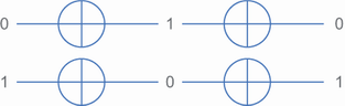
This process is reversible. If the value of a qubit is 1 after a Pauli-X gate has been applied, we know that it had the value of 0 before the gate was applied. If, on the other hand, the end value is 0, we know that the original value was 1. Hence, the principle of reversible gates holds so far. By applying a second Pauli-X gate after applying the first Pauli-X gate, we store the original state of the system, as illustrated in figure 3.8.

3.5 Playing with qubits in Strange

We haven’t discussed superposition and entanglement yet, and our introduction to qubits was basic. The real power of QC will be demonstrated when we explain the concepts of superposition and entanglement. At this point, however, we can already create a simple application using Strange to see the Pauli-X gate in action.

In chapter 2, we used the high-level API of Strange to create an application that uses a quantum algorithm to return random values. In the following demo, we use the low-level API of Strange and work directly with qubits and gates. The code in listing 3.1 creates a single qubit (which has the initial value of 0), applies the Pauli-X gate, and measures the resulting value.

Tip The source code for this demo can be found in the ch03/paulix directory in the example repository. See appendix A for more information on how to obtain the example code.

Listing 3.1 Java application using a Pauli-X gate

public static void main(String[] args) {
    QuantumExecutionEnvironment simulator =
        new SimpleQuantumExecutionEnvironment();     ❶
    Program program = new Program(1);                ❷
    Step step = new Step();
    step.addGate(new X(0));
    program.addStep(step);
    Result result = simulator.runProgram(program);   ❸
    Qubit[] qubits = result.getQubits();
    Qubit zero = qubits[0];
    int value = zero.measure();
    System.out.println("Value = "+value);            ❹
}

❶ Creates an Environment for declaring and executing a quantum application

❷ Defines a Program

❸ After the Program is defined, it can be executed on the Environment and a Result can be obtained.

❹ The Result can be processed and returned to the user.

Now let’s run the code:

mvn javafx:run

As expected, the output of the program is as follows:

Value = 1

In this code, we introduce a number of concepts encountered in Strange. We talk about an execution environment, a program consisting of steps, and some results. Note that those concepts are typically used in all kinds of QC simulators and editors.

3.5.1 The QuantumExecutionEnvironment interface

The physical location and conditions of where and how a quantum application is executed are not relevant to the developer, and the options are still evolving. There are already cloud services offering real quantum infrastructure (such as IBM and Rigetti), but it is also possible to assume that a quantum co-processor will be able to execute quantum applications. Today, most quantum applications are executed on quantum simulators, which can run either locally or in a cloud environment. In summary, multiple different execution environments are capable of executing quantum applications.

Strange abstracts the differences in execution environments and provides an interface, QuantumExecutionEnvironment, in the org.redfx.strange package that provides the API for quantum applications to interact with the execution environment. Strange contains several implementations of QuantumExecutionEnvironment, but the most important thing is that quantum applications written with Strange can run on all current and future implementations without being modified.

The simplest execution environment uses a built-in simulator and is instantiated as follows:

QuantumExecutionEnvironment simulator = new
SimpleQuantumExecutionEnvironment();

SimpleQuantumExecutionEnvironment in the org.redfx.strange.local package provides a quantum simulator that executes quantum operations using classical software. Clearly, it is slower than real hardware, and because quantum simulators are memory-hungry when dealing with large numbers of qubits, it is not recommended for use with lots of qubits. For the demos in this book, SimpleQuantumExecutionEnvironment is more than good enough.

3.5.2 The Program class

If you want to create a quantum application in Strange, you have to create a new instance of Program. The Program class is in the org.redfx.strange package, and it provides an entry point to quantum applications you want to write.

The Program constructor requires a single integer parameter, defining the number of qubits you will use in the application. In the case of our simple application, we will use a single qubit, which explains this line:

Program program = new Program(1)

3.5.3 Steps and gates

A quantum Program is composed of one or more steps operating on the qubit. Each step is defined by an instance of Step. The Step class is in the org.redfx.strange package as well and has a zero-argument constructor. Inside a step, you define which gates are used.

In our example, we have a single step that is created like this:

Step step = new Step()

The step is further defined by adding a gate. Here we use the Pauli-X gate, which is defined by the X class in the org.redfx.strange.gate package. The constructor of the Pauli-X gate requires one integer to be passed, which is the index of the qubit the gate is acting on. In this case, because we have a single qubit, the index is 0. Creating this gate and adding it to the Step instance is done as follows:

step.addGate(new X(0));

In a single step, each qubit may be affected by no more than one gate. A gate may act on more than one qubit, but two gates in the same step cannot act on the same qubit. The following code snippet is wrong, as we add two gates to the same step, and both gates operate on the same qubit (with index 0):

step.addGate(new X(0));
step.addGate(new H(0));

If you try to use this snippet in an application, Strange will throw an IllegalArgumentException with the message “Adding gate that affects a qubit already involved in this step.”

Note that we introduced another gate here: the Hadamard gate, represented by the H class. We cover this gate in the next chapter; we use it here only to show that it is not allowed to have two gates operating on the same qubit in a single step.

At this point, the single execution step in our program is ready. We have to instruct the Program instance that our Step instance should be added to the program:

program.addStep(step);

3.5.4 Results

When a quantum application or a Program has been executed, a result can be obtained. We briefly mentioned that a qubit can be in a so-called superposition, but that once it is measured, it will hold the value 0 or the value 1. Therefore, it is impossible to have intermediate results in quantum applications. Quantum simulators that are not using real physical qubits do not have this restriction, though; for debugging purposes, intermediate values can be used and can be useful, as we will demonstrate in chapter 7.

Strange defines the Result class in the org.redfx.strange package, and instances of it are created by the execution environment. The result is returned when the runProgram() method is called on the QuantumExecutionEnvironment:

Result result = simulator.runProgram(program);

The resulting instance of the Result class contains information about the final state of the quantum system. We talk about this in more detail in the following chapters. For now, we are interested only in the status of the single qubit that is in our system.

The Result class contains a method to retrieve the qubits:

Qubit[] qubits = result.getQubits();

Because we have only one qubit in the system, it can be obtained as follows:

Qubit zero = qubits[0];

We can ask for the value of this qubit after the program has been executed:

int value = zero.measure();

Finally, we print the value using simple Java commands:

System.out.println("Value = "+value);

Initially, qubits are in the 0 state. Our simple application sends the qubit through a Pauli-X gate and then measures the new value, which is always equal to 1. For some algorithms, you want a qubit to be in the 1 state initially: this is easily achieved by using a Pauli-X gate as the first step of the algorithm.

3.6 Visualizing quantum circuits

The code in the previous example is not hard to understand and follow, but it represents a simple quantum circuit involving only a single qubit and a single gate. When applications become more complex, it can be difficult to read the code and have a clear understanding of what is happening. Many quantum simulators or applications that allow us to generate quantum applications come with a visualization tool.

The Strange library has a companion library called StrangeFX that allows us to render programs intuitively. StrangeFX is written in Java as well, and it uses JavaFX, the standard Java UI Platform, for rendering. The paulixui example in this chapter’s code shows this library in action.

When you have a Program, visualizing it is very easy. In case you are using the Maven build system, including the StrangeFX library is straightforward. We need to add two new dependencies in the pom.xml file:

<dependency>
  <groupId>org.openjfx</groupId>
  <artifactId>javafx-controls</artifactId>    ❶
  <version>15</version>
</dependency>
<dependency>
  <groupId>org.redfx</groupId>
  <artifactId>strangefx</artifactId>          ❷
  <version>0.0.10</version>
</dependency>

❶ The javafx.controls module allows us to create graphical control components. This module depends on a few other javafx modules, which are loaded transitively.

❷ Retrieves the org.redfx.strangefx artifact. It contains the code required to visualize quantum circuits.

The situation is similar when you are using the Gradle build system. You have to modify the build.gradle file and add a dependency to StrangeFX, like this:

plugins {
    id 'application'
    id 'org.openjfx.javafxplugin' version '0.0.10'    ❶
}
 
repositories {
    mavenCentral();
    jcenter();
}
 
dependencies {
    compile 'org.redfx:strange:0.0.17'
    compile 'org.redfx:strangefx:0.0.10'              ❷
}
 
javafx {
    modules = [ 'javafx.controls' ]                   ❸
}
 
mainClassName = 'org.redfx.javaqc.ch03.paulixui.Main'

❶ Adds the JavaFX plugin for Gradle

❷ Depends on StrangeFX

❸ Uses the javafx.control module in the application

Note that we added this line to the plugins section:

id 'org.openjfx.javafxplugin' version '0.0.10'

This plugin makes sure that all the code required for running the JavaFX application can be used. Further, we have to add the dependency to StrangeFX to the list of dependencies:

compile 'org.redfx:strangefx:0.0.10'

Finally, because our application uses the JavaFX controls module, we have to tell the Java system to load it:

javafx {
    modules = [ 'javafx.controls' ]
}

The code required for rendering a program is simple. StrangeFX contains an org.redfx.strangefx.render.Renderer class that has the following static method:

Renderer.renderProgram(Program program);

This method analyzes the program and creates a visual representation of it in which each qubit is represented on a line. The initial state, with all qubits in the |0〉 state, is on the left. Going to the right, quantum gates are pictured when they are encountered. At the end of the line, the probability of this gate being measured with 1 is shown. Hence, if we want to render the circuit we composed before, we have to modify the end of our application as follows:

    int value = zero.measure();
        System.out.println("Value = "+value);
        Renderer.renderProgram(program);
    }

Running this program renders the user interface shown in figure 3.9. In this diagram, the visual components refer to the different components of the application, as we’ve marked.

Summary

• The fundamental concepts of quantum computing are qubits (or quantum bits) and quantum gates.

• There are similarities and differences between those concepts and their counterparts in classical computing.

• The state of a qubit can be expressed in different notations: Dirac notation or a vector notation.

• Using the Java-based Strange quantum simulator, quantum gates can be composed into a quantum application.

• The Pauli-X gate is one of these quantum gates, and it can be used in a quantum application.