
9 Deutsch-Jozsa algorithm
- Obtaining information from classical functions
- Function evaluations vs. function properties
- Quantum gates that correspond to classical black box functions
- Understanding the Deutsch algorithm and the Deutsch-Jozsa algorithm
The Deutsch-Jozsa algorithm that we discuss in this chapter demonstrates some of the characteristics of typical quantum algorithms. The direct practical use cases may be limited, but the algorithm is a great tool for explaining the logic that quantum algorithms often follow.
9.1 When the solution is not the problem
Do you know if the number 168,153 can be divided by 3? There are a number of ways to find out. For example, you can simply take a calculator and obtain the result:
The result of the division is 56,051. But that was not the question. Actually, we don’t care about this result. But thanks to this evaluation, we know the real answer: there are no digits after the decimal point, so we can conclude the number can indeed be divided by 3.
There is another simple approach to find the answer to this question, and you might know this simple trick: take the sum of the individual digits that compose the number, and see if that sum can be divided by 3. If so, the original number can be divided by 3 as well. Let’s do that:
Since 24 can be divided by 3, we can conclude that 168,153 can also be divided by 3.
The first approach (using the calculator) gave us a result of a division, and it provided us with the real answer. The second approach (sum of the individual digits) only provided the real answer, not the outcome of the division.
The relevance of this is that in many cases, we are interested in a specific property of something (e.g., a number or a function). We are not interested in a function evaluation, but we somehow want to obtain information about the function. Evaluating the function is often the easiest way to do so, but it can be more efficient to indirectly look at the properties of the function and draw conclusions from there.
This is of particular interest in quantum computing. A quantum computer with n qubits that needs to examine a specific function can only do one function evaluation at a time. Applying the quantum circuit to a given specific set of input qubits will result in a modified state of these qubits. Measuring them gives a particular result, and if you want a new result, you need to run the circuit again. Even though we can apply Hadamard gates to the input qubits to bring them into superposition—which allows us to evaluate the qubits in the 0 and 1 states simultaneously—we can’t magically create new qubits that will hold the information of the different cases. This is shown in figure 9.1 for a system with two qubits.

Figure 9.1 A quantum system with two qubits can do many evaluations, but only two qubits can be measured.
The internal computations can contain the equivalent of many evaluations, but we can’t obtain those simultaneously. We are limited to a result of n qubits. But that is often enough to solve problems. In the case of our number being a multiplicator of 3 or not, a single qubit is enough to store the answer. We don’t need to evaluate the division function.
In this chapter, we demonstrate this approach using quantum computing. We investigate a property of a function f acting on n bits, without being interested in the individual function evaluations. We show that retrieving the property in the classical way requires 2n–1 + 1 function evaluations. With the quantum algorithm, the property can be obtained with a single evaluation.
The functions we use are very simple, and there is no direct use case for this problem. But it demonstrates an essential aspect of quantum computing, and it explains why quantum computing is often associated with “exponential” complexity. You can easily see that the more input bits the function has, the harder it becomes to solve the problem in a classical way. The number n is indeed in the exponent, and as we showed in chapter 1, exponential functions quickly result in huge values. If a quantum algorithm can fix the same problem in just a single evaluation (or, in general, in less than an exponential number of equations), this is a huge advantage for a quantum computer.
We will gradually come to the algorithm that achieves this. We will follow the approach shown in figure 9.2.
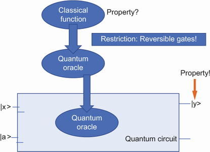
First we talk about properties of functions and how to obtain them in a classical way. Next, we convert the functions into quantum blocks called oracles. We show that there are some requirements for doing this. Once we can create a quantum oracle that represents a classical function, this oracle can be used in a quantum circuit. Evaluating this quantum circuit once results in the property of the function we are looking for.
9.2 Properties of functions
In most typical cases where functions are involved, you are interested in finding the result of a function. For example, consider the function y(x) = x2.
If we want to know the value of this function for, for example x = 4 and x = 7, we need to evaluate this function:
y(7) = 72 = 49
In some cases, though, the function evaluations are not important, but the characteristics of the functions are. In this area, quantum algorithms can be helpful. An example that we will discuss in chapter 11 is the periodicity of a function. We are not interested in the individual evaluations of a function, but we are interested in the periodicity. A periodic function is a function where the same pattern of values comes back with a fixed periodicity. Here’s an example:
From this table, you can tell that the function has a periodicity of 3: for every value of x, the result of the function is the same as the function applied to x + 3. This is an example where the property of a function can be more interesting than the function evaluations themselves.
9.2.1 Constant and balanced functions
In general, the functions we consider are noted as f(x), where f is the function that operates on an input variable called x. The evaluation of a function for a specific input is also called the result and sometimes noted as y, where y = f(x).
In this chapter, we start with a very simple family of functions that have simple properties. We start with a function with only a single input bit, and we extend it later to a function with n input bits. In all cases, the result of the function is either 0 or 1.
The functions we discuss here have a special property: they are either balanced functions or constant functions. A function is called constant when the result is not dependent on the input. In our case, that means the result is either 0 for all input cases or 1 for all input cases. A function is called balanced when the result is 0 in 50% of the cases and 1 in the other cases.
The Deutsch algorithm, which we discuss shortly, deals with a function called f that takes a single bit (a Boolean value) as its input and produces a single bit as well. The function only operates on 0 and 1, and its result is either 0 or 1. The combination of two input options and two output options leads to four possible cases for this function, which we name f1, f2, f3, and f4:
From those definitions, it appears that f1 and f4 are constant functions, and f2 and f3 are balanced functions.
In many classical algorithms, it is important to know the output of a function for specific values. In many quantum algorithms, on the other hand, it is useful to know the properties of the function under consideration.
This is part of the “different thinking” that is required when considering quantum algorithms. Thanks to superposition, a quantum computer can evaluate many possibilities simultaneously; but since obtaining a result requires a measurement, the superposition is gone, and we are back to a single value. Hence, the added value is in the function evaluation and not in the result of the function evaluation.
In the Deutsch algorithm, a function is provided, but we don’t know what function it is. We know it is f1, f2, f3, or f4, but that’s all we know. We are now asked to find out if this function is constant or balanced. Our task is not to determine whether the provided function is f1, f2, f3, or f4. We are asked about a property of the function, not the function itself. Schematically, the problem is explained in figure 9.3.

How many function evaluations do we need before we can answer this question with 100% certainty? If we do only a single evaluation (we only calculate either f(0) or f(1)), we don’t have enough information.
Suppose we measure f(0) and the result is 1. From the earlier table, it seems that, in this case, our function is either f3 (which is balanced) or f4 (which is constant). So, we don’t have enough information. If the result of measuring f(0) is 0, the table shows that the function is either f1 (which is constant) or f4 (which is balanced). Again, this proves that measuring f(0) is not enough to conclude whether the function is constant or balanced. It can be either.
It turns out we need two classical function evaluations before we can determine whether the provided function is constant or balanced. Let’s write a Java application that demonstrates this. You can find this application in the ch09/function directory of the examples.
Listing 9.1 Two evaluations to declare a function constant or balanced
static final List<Function<Integer, Integer>> functions = new ArrayList<>();

    static {
        Function<Integer, Integer> f1 = (Integer t) -> 0;                ❶
        Function<Integer, Integer> f2 = (Integer t) -> (t == 0) ? 0 : 1;
        Function<Integer, Integer> f3 = (Integer t) -> (t == 0) ? 1 : 0;
        Function<Integer, Integer> f4 = (Integer t) -> 1;
        functions.addAll(Arrays.asList(f1, f2, f3, f4));
    }

    public static void main(String[] args) {
        Random random = new Random();
        for (int i = 0; i < 10; i++) {                                   ❷
            int rnd = random.nextInt(4);
            Function<Integer, Integer> f = functions.get(rnd);           ❸
            int y0 = f.apply(0);                                         ❹
            int y1 = f.apply(1);
            System.err.println("f" + (rnd + 1 + " is a "                 ❺
                    + ((y0 == y1) ? "constant" : "balanced")
                    + " function"));
        }
    }
❶ Prepares the four possible functions. This step needs to be done only once.
❸ Picks a random function, not knowing anything about its implementation
❹ Performs two function evaluations: one for input 0 and one for input 1
❺ If the results of those two evaluations are similar, the function is constant; otherwise, the function is balanced.
In this code, we create the four possible functions in a static block. We do this is because we want to stress that the creation of the function and the determination of whether they are constant or balanced should be considered two independent processes.
After the functions are created, the application really starts. Inside the for loop, a random function is picked. Based on the two function evaluations, we can determine whether the function is constant or balanced.
A possible output of this application is the following:
f4 is a constant function
f4 is a constant function
f3 is a balanced function
f1 is a constant function
f2 is a balanced function
f2 is a balanced function
f1 is a constant function
f4 is a constant function
f3 is a balanced function
f2 is a balanced function
As expected, the application has the correct answers for every loop. But in every loop, we performed two evaluations of the function. As we showed earlier, a single evaluation would not be sufficient to conclude whether the function is balanced.
9.3 Reversible quantum gates
So far, we have talked about classical functions and their properties. Before we can discuss the quantum equivalent of those functions, we need to look into the requirement of quantum gates in more detail.
In the previous chapters, you learned about and used several quantum gates. These gates have many similarities with gates you encounter in classical computing. However, there are some fundamental differences.
Quantum gates are physically achieved using properties of quantum mechanics, and therefore they must obey the requirements and restrictions that are related to quantum mechanics. One of the key requirements for a quantum gate is that it should be reversible. This means when a quantum gate is applied to a given begin status, there should exist another quantum gate that brings the result back to the begin status. In a quantum system, information can’t simply disappear. The information that was in a system before a specific quantum gate is applied should be recoverable. We briefly touched on the concept of reversible gates in chapter 7. Since this is such an important concept, we’ll go a bit deeper into the topic now.
All the gates we have discussed so far are reversible. Let’s show that with a simple example: the Pauli-X gate. The gate that brings a system back to its original state after a Pauli-X gate is applied is another Pauli-X gate. We can explain this in two ways:
9.3.1 Experimental evidence
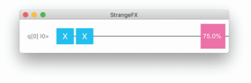
Let’s create a simple quantum application that applies a Pauli-X gate on a single qubit, followed by another Pauli-X gate. Instead of only taking the special cases into account where the qubit is either |0> or |1>, we will artificially initialize the qubit so that it has a 75% chance of being measured as 1. The circuit is shown in figure 9.4.
The code for this example can be found in the example repository under ch09/ reversibleX. The relevant code is shown next.
Listing 9.2 Two Pauli-X gates applied to a single qubit
QuantumExecutionEnvironment simulator =
                new SimpleQuantumExecutionEnvironment();
        Program program = new Program(1);                ❶
        Step step0 = new Step();                         ❷
        step0.addGate(new X(0));

        Step step1 = new Step();                         ❸
        step1.addGate(new X(0));
        program.addStep(step0);                          ❹
        program.addStep(step1);
        program.initializeQubit(0,.5);                   ❺

        Result result = simulator.runProgram(program);   ❻
        Renderer.showProbabilities(program,1000);        ❼
        Renderer.renderProgram(program);
❶ Creates a quantum application with a single qubit
❷ The first step (step0) applies a Pauli-X gate to the qubit.
❸ The second step (step1) applies another Pauli-X gate to the qubit.
❹ Adds the steps to the quantum program
❺ Initializes the single qubit with an alpha value of 0.5, which leads to a probability of 25% of measuring 0
❻ Executes the quantum program
❼ Renders the statistical results of running this program 1,000 times
The result of running this circuit 1,000 times is shown in figure 9.5. As expected, after applying two Pauli-X gates, the probability of measuring 0 is about 25%, and there is about a 75% chance of measuring 1. This matches the artificial initial value that we applied to the qubit.

9.3.2 Mathematical proof
In chapter 4, we explained the mathematical equivalent of applying a gate to a qubit: we multiply the gate matrix and the probability vector of the qubit. Let’s assume the initial qubit is described as follows:
|
|

Applying two Pauli-X gates to this qubit brings it into the following state

where X is the matrix defining the Pauli-X gate. From chapter 4, we know the structure of the matrix, so we can write

Using matrix multiplication (explained in appendix B), we can write this as follows:
|
|

From equation 9.2, it can be seen that the end state of the qubit, denoted by ψ, is written as

This is exactly the same as the begin state of the qubit, which was shown in equation 9.1.
This shows that after applying two Pauli X-gates, the quantum system is in the exact same state as in the beginning—before the two Pauli-X gates were applied. Hence, we have proven that the Pauli-X gate is indeed a reversible gate, and that the changes to a quantum system caused by applying a Pauli-X gate can be undone by applying another Pauli-X gate. Now that you have learned that the Pauli-X gate is a reversible quantum gate, you can use the same technique to prove that the other gates you have learned about are reversible as well.
Note The gates we’ve introduced so far have the special property that they are their own inverse. This is not always true, and there is no restriction that a quantum gate should be its own inverse.
9.4 Defining an oracle
In many quantum algorithms, the term oracle is used. We will use an oracle when we create the Deutsch algorithm, so some explanation is needed now.
An oracle is used to describe a quantum black box—similar to how each of the earlier functions (f1, f2, f3, and f4) can be described as a classical black box. Internally, the functions had some computational flow; but in the main loop of the program, we pretended we didn’t know about the internals—we simply evaluated the functions for different input values.
The same concepts can be applied to an oracle. Internally, an oracle is composed of one or more quantum gates, but we typically don’t know which gates. By querying the oracle (e.g., by sending input and measuring the output), we can learn more about the properties of the oracle. Because an oracle is composed of quantum gates, the oracle itself also needs to be reversible.
An oracle can thus be considered the quantum equivalent of the black-box functions we discussed earlier in this chapter. Both an oracle and a function perform some calculations, but we don’t know the internal details about these calculations. This is shown in figure 9.6.

Figure 9.6 A quantum oracle, acting as a black box in a quantum circuit, is internally composed of a number of gates.
Let’s look at an example of an oracle used in a simple quantum application. Using the Strange simulator, you define an oracle by providing the matrix that is the mathematical representation of the oracle. That sounds like we are cheating: are we really defining something that we later claim we don’t know anything about? The answer is yes. We indeed create this oracle, since someone has to do it. In real quantum applications, the oracle is an external component given to us.
Note The creation of the function and the creation of the oracle should be considered totally separated processes. In the upcoming algorithms, we assume that someone created an oracle for us. The algorithm itself has no clue how the oracle was created, how complex or simple it is, etc. This is often confusing, since to demonstrate the algorithm, we obviously need an oracle. However, the complexity of creating the oracle should not be considered part of the complexity of the algorithm. Just assume that someone (yourself, another developer, a real piece of hardware, or nature itself) created the oracle and provided it to you.
We learned before that all gates can be represented by a matrix. An oracle contains zero or more gates, and therefore the oracle itself can also be represented by a matrix. An oracle can be considered part of the quantum circuit that is given to you. You can’t see the gates that together constitute the oracle, but you can use them in your quantum programs.
In Strange, an oracle is defined by providing the matrix that represents it. In a real hardware situation, the oracle is available as is. In a software simulation, we somehow need to define the oracle’s behavior, so a matrix needs to be provided. Figure 9.7 shows how an oracle can be part of a quantum program.
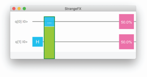
Figure 9.7 An oracle, pictured as a vertical box, is used in this quantum circuit. First a Hadamard gate is applied, followed by the oracle.
We will create some code in which we apply an oracle in a quantum program. We create the oracle by providing a matrix that may look familiar to you. It is recommended that you not look at the contents of the matrix, though, as doing so takes away the mystery of the oracle. Instead, you can look at the result of the entire program and try to find out what the oracle is doing.
Let’s consider the following snippet, which is taken from the example in ch09/oracle.
Listing 9.3 Introducing an oracle in quantum applications
QuantumExecutionEnvironment simulator =
           new SimpleQuantumExecutionEnvironment();
    Program program = new Program(2);                ❶
    Step step1 = new Step();
    step1.addGate(new Hadamard(1));                  ❷


    Complex[][] matrix =  new Complex[][]{           ❸
            {Complex.ONE,Complex.ZERO,
                  Complex.ZERO,Complex.ZERO},
            {Complex.ZERO,Complex.ONE,
                  Complex.ZERO,Complex.ZERO},
            {Complex.ZERO,Complex.ZERO,
                   Complex.ZERO,Complex.ONE},
            {Complex.ZERO,Complex.ZERO,
                   Complex.ONE,Complex.ZERO}
    };

    Oracle oracle = new Oracle(matrix);              ❹

    Step step2 = new Step();                         ❺
    step2.addGate(oracle);

    program.addStep(step1);                          ❻
    program.addStep(step2);

    Result result = simulator.runProgram(program);   ❼
    Renderer.showProbabilities(program,1000);
    Renderer.renderProgram(program);
❶ Creates a quantum program that requires two qubits
❷ The first step applies a Hadamard gate to the second qubit.
❸ Creates a matrix containing complex numbers. For now, we don’t interpret these numbers.
❹ Creates an oracle based on this matrix
❺ Creates a second step in which the oracle is applied
❻ Adds both steps to the quantum program
❼ Executes the program and displays its circuit and the results of 1,000 runs
The circuit created here is the one shown in figure 9.7. The result of running this circuit 1,000 times is shown in figure 9.8.

If you look at those statistical results, it seems that there are only two possible outcomes: |00> or |11>. Remember from chapter 5 that a circuit with two entangled qubits has the same probabilities: there is a 50% of measuring |00> and a 50% chance of measuring |11>. This is an indication that the oracle we created, combined with the initial Hadamard gate, results in two entangled qubits. In chapter 5, you created two entangled qubits by applying a CNot gate after a Hadamard gate. So, we learn that the oracle we created behaves like a CNot gate. If we cheat and look at the contents of the oracle, we see that the matrix that represents the oracle matches the matrix of the CNot gate. This exercise shows that we can apply oracles to a quantum circuit. We can apply an oracle without knowing its internal details.
9.5 From functions to oracles
In the Deutsch algorithm, we show that a single evaluation is enough to find out if a provided function is constant or balanced. Before we can do that, we need to convert the classical function into a quantum operation.
We can’t simply apply a function to a qubit. Remember, we explained that all quantum gates need to be reversible. A function that, after being applied, makes it impossible to retrieve the original input can’t be used in a quantum circuit. Therefore, the function first needs to be transformed into a reversible oracle.
In this section, we demonstrate how oracles can be created that can then be used in the Deutsch algorithm we explain in the next section. Similar to how a classical function is handed to the classical algorithm, an oracle is handed to the quantum algorithm.
Every classical function that we described earlier in this chapter can be represented by a specific oracle. Since we had four possible functions, we also have four possible oracles.
The general way to construct an oracle based on a function is shown in figure 9.9. In this approach, we have an input qubit called |x> and an additional qubit named |a>.

The oracle leaves the |x> qubit in its original state, and the |a> qubit is replaced by the XOR operation between a and f(x). Let’s examine this oracle in a bit more detail: we will investigate what it looks like for the four functions we defined earlier.
9.5.1 Constant functions
The first function, f1, is a constant function that returns 0 regardless of the input. Hence, since f(x) = 0 for any value of x, the output status of the second qubit can be simplified as follows:
The resulting oracle can be pictured as in figure 9.10. In this case, the oracle is simply the Identity matrix. Both |x> and |a> are unaltered between the input and the output. The hidden logic inside the oracle can thus be represented by the scheme in figure 9.11.


As a result, the matrix representing the oracle is written as follows:

This matrix is an Identiy matrix: it does not alter the probabilities when measuring the qubits. Multiplying this matrix with any probability vector yields the original probability vector.
Note The circuit shown in figure 9.11 isn’t the only possible circuit that results in the Identity matrix. Many other circuits operate on two qubits and return the two qubits in the same state. For example, applying two Pauli-X gates on each qubit results in the exact same state. This is part of the black-box aspect of an oracle: we don’t know the internal details, and we are typically not interested in those. We want to investigate a specific property of the oracle, not its internal implementation.
The fourth function, f4, is a constant function that always returns the value 1, regardless of the input. As a consequence, the output of the second qubit after applying the oracle can be written as follows:
a ⊕ f(x) = a ⊕ 1 = ā
The horizontal bar above a variable indicates that this is the inverted variable, which in this case corresponds to a Pauli-X gate being applied to |a>. So, this oracle can be schematically presented as shown in figure 9.12.


9.5.2 Balanced functions
Let’s have a look at the second classical function, f2. This function is defined as follows:
f(0) = 0
f(1) = 1
This can also simply be written as f(x) = x.
Using this in the general description of the oracle, as shown in figure 9.9, the scheme simplifies to figure 9.13.

This is exactly the state that would be obtained if the oracle had a CNot gate. Hence, a possible circuit for the oracle corresponding to the f2 function is shown in figure 9.14.

The matrix representation of this oracle is, thus, also the matrix representation of the CNot gate:

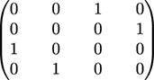
9.6 Deutsch algorithm
The Deutsch algorithm requires only a single evaluation of the oracle to know whether the function under consideration is constant or balanced. Let’s start with a naive approach and assume that all we need to do is apply the oracle and measure the result.
The code for this is in ch9/applyoracle. Before we explain the algorithm, we first point to the part of the code where the different oracles are created. As we stated before, the creation of an oracle is not part of the algorithm that tries to find out whether a function is balanced. Although for practical reasons, we create the oracle in the same Java class file as the algorithm, it should be stressed that the creator of the oracle (who might know the outcome of the problem) and the creator of the algorithm are not the same.
From the previous section, it should be clear that there are four different types of oracles. An infinite number of oracles can be used to represent the simple functions we discussed at the beginning of this chapter, but they all corresponds to one of the four gate matrices that we showed in the previous section. The algorithm will ask to pick a random oracle, and the code that constructs this random oracle is as follows.
Listing 9.4 Creating an oracle
static Oracle createOracle(int f) {                   ❶
    Complex[][] matrix = new Complex[4][4];           ❷

    switch (f) {
        case 0:                                       ❸
            matrix[0][0] = Complex.ONE;
            matrix[1][1] = Complex.ONE;
            matrix[2][2] = Complex.ONE;
            matrix[3][3] = Complex.ONE;
            return new Oracle(matrix);
        case 1:                                       ❹
            matrix[0][0] = Complex.ONE;
            matrix[1][3] = Complex.ONE;
            matrix[2][2] = Complex.ONE;
            matrix[3][1] = Complex.ONE;
            return new Oracle(matrix);
        case 2:                                       ❺
            matrix[0][2] = Complex.ONE;
            matrix[1][1] = Complex.ONE;
            matrix[2][0] = Complex.ONE;
            matrix[3][3] = Complex.ONE;
            return new Oracle(matrix);
        case 3:                                       ❻
            matrix[0][2] = Complex.ONE;
            matrix[1][3] = Complex.ONE;
            matrix[2][0] = Complex.ONE;
            matrix[3][1] = Complex.ONE;
            return new Oracle(matrix);
        default:                                      ❼
            throw new IllegalArgumentException("Wrong
                                index in oracle");
    }
}
❶ When this function is called, an integer needs to be provided indicating what oracle type to return.
❷ In all cases, the result is a 4 × 4 matrix of complex numbers.
❸ If the caller provides 0, an oracle with the matrix corresponding to f1 will be returned.
❹ If the caller provides 1, an oracle with the matrix corresponding to f2 will be returned.
❺ If the caller provides 2, an oracle with the matrix corresponding to f3 will be returned.
❻ If the caller provides 3, an oracle with the matrix corresponding to f4 will be returned.
❼ If we reach here, the caller provided a wrong value, and we throw an exception.
Now that we have the code that returns an oracle corresponding to a value we provide, we can focus on the algorithm that should detect whether the oracle is linked with a constant function or a balanced function.
We start with the naive approach where we just apply the oracle to two qubits that are initially 0. We hope the result will tell us with 100% confidence whether the underlying function is balanced.
Listing 9.5 Applying the oracle
static void try00() {                                    ❶
    QuantumExecutionEnvironment simulator =
            new SimpleQuantumExecutionEnvironment();
    Program program = null;
    for (int choice = 0; choice < 4; choice++) {         ❷
        program = new Program(2);                        ❸

        Step oracleStep = new Step();                    ❹
        Oracle oracle = createOracle(choice);
        oracleStep.addGate(oracle);
        program.addStep(oracleStep);

        Result result = simulator.runProgram(program);   ❺
        Qubit[] qubits = result.getQubits();

        boolean constant =
                  (choice == 0) || (choice == 3);        ❻

        System.err.println((constant ? "C" : "B") +
             ", measured = |" + qubits[1].measure() +
             " , " + qubits[0].measure()+">");
    }
}
❶ This function is called try00 as it applies the oracles to two qubits that are in their initial state of |0>.
❷ Iterates over the four possible oracle types
❸ Creates a quantum program that contains two qubits
❹ Creates the oracle corresponding to the loop index “choice” and adds it to the program
❺ Executes the program and obtains the results
❻ Based on the loop index “choice,” we know if the oracle corresponds to a balanced or constant function. We print that information together with the measurements of the two qubits.
The results of this application are as follows:
Note that since we didn’t use superposition, these results are always the same.
Let’s investigate these results. There are two possible outcomes we can measure: the result is either |00> or |10>. Unfortunately, a single result doesn’t tell us whether the function was constant (as indicated by the C) or balanced (as indicated by the B). For example, if we measure |00>, the function is either f1 or f2; but since the first is constant and the second is balanced, we don’t have an answer to our question.
We can be clever and try to run the application again, but this time we first flip one of the qubits, or both, to the |1> state using a Pauli-X gate. This is shown in the code in the same file; it is a good exercise to create this code yourself before looking at the example.
Doing so, we run four versions of our simple program, each corresponding to a different initial state of the two qubits. The results are shown here:
Use |00> as input
C, measured = |00>
B, measured = |00>
B, measured = |10>
C, measured = |10>

Use |01> as input
C, measured = |01>
B, measured = |11>
B, measured = |01>
C, measured = |11>

Use |10> as input
C, measured = |10>
B, measured = |10>
B, measured = |00>
C, measured = |00>

Use |11> as input
C, measured = |11>
B, measured = |01>
B, measured = |11>
C, measured = |01>
If you analyze this result, you will conclude that none of those versions is sufficient to detect whether the oracle corresponds to a constant or a balanced function by doing a single evaluation.
But so far, we didn’t use the powerful superposition. We will do that now. Before we write the code for the algorithm, figure 9.15 shows the quantum circuit that leads to the result.

We start with two qubits. The first qubit, q[0], will be evaluated. But instead of evaluating twice, the first time in the state |0> and the second time in the state |1>, we apply a Hadamard transform to it to bring it into a superposition. You can think of this as allowing us to evaluate both possible values in a single quantum step.
The second qubit, q[1], which is initially |0> as well, is first flipped into |1> by applying a Pauli-X gate. Next, a Hadamard gate is applied to this qubit. Both qubits are then used as input to the oracle we discussed in the previous section. After the oracle has been applied, we discard the second qubit. On the first qubit, a Hadamard gate is applied, and the qubit is measured.
Now we arrive at the great thing about this algorithm. The following statement can be mathematically proven: If the measurement is 0, we are guaranteed that the function represented by the oracle is balanced. If the measurement is 1, we know the considered function is constant.
If you are interested in the mathematics behind this, it can be proven mathematically that the probability of measuring 0 for the first qubit after the circuit is applied is given by

If f is a constant function, this will always result in 1. If f is a balanced function, this will always result in 0.
Instead of proving this, we will create code that runs the circuit for the four different functions and measure the output to see if our statement is correct. The interesting part of this algorithm is that we managed to make the first qubits dependent on the evaluation of all values. We don’t have the measurements for all these evaluations, but that was not the original question. The original goal was to determine whether a given function is constant or balanced.
The following code implements the algorithm. It is taken from the ch09/deutsch example:
QuantumExecutionEnvironment simulator =
            new SimpleQuantumExecutionEnvironment();
    Random random = new Random();
    Program program = null;
    for (int i = 0; i < 10; i++) {                       ❶
        program = new Program(2);                        ❷
        Step step0 = new Step();
        step0.addGate(new X(1));                         ❸

        Step step1 = new Step();                         ❹
        step1.addGate(new Hadamard(0));
        step1.addGate(new Hadamard(1));

        Step step2 = new Step();
        int choice = random.nextInt(4);
        Oracle oracle = createOracle(choice);            ❺
        step2.addGate(oracle);                           ❻

        Step step3 = new Step();
        step3.addGate(new Hadamard(0));                  ❼

        program.addStep(step0);                          ❽
        program.addStep(step1);
        program.addStep(step2);
        program.addStep(step3);
        Result result = simulator.runProgram(program);   ❾
        Qubit[] qubits = result.getQubits();             ❿
        System.err.println("f = " + (choice+1) +
              ", val = " + qubits[0].measure());
    }
❶ The loop will be executed 10 times, each time with a random oracle.
❷ Creates a program with two qubits
❸ The first step applies a Pauli-X gate to the second qubit.
❹ The second step applies Hadamard gates to both qubits.
❺ Chooses a random oracle (from a predefined list)
❻ Adds the oracle to the quantum circuit
❼ Applies another Hadamard gate to the first qubit
❽ Adds the steps to the quantum program
❾ Executes the quantum program
❿ The first qubit is measured, and, based on its value, we know whether the oracle corresponded with a constant or balanced function.
If you run this application, you will see the circuit, and the console will show output similar to the following:
f = 3, val = 1
f = 3, val = 1
f = 3, val = 1
f = 1, val = 0
f = 4, val = 0
f = 4, val = 0
f = 2, val = 1
f = 1, val = 0
f = 2, val = 1
f = 4, val = 0
For every line in this output, the type of function is printed (f1, f2, f3, or f4) followed by the measured value of the first qubit. As you can see, this value is always 1 for f2 and f3 (the balanced functions), and it is 0 for f1 and f4 (the constant functions).
9.7 Deutsch-Jozsa algorithm
The Deutsch algorithm shows that a specific problem that requires two evaluations in a classical approach can be solved by a single evaluation using a quantum algorithm. While this may sound a bit disappointing, the principle is very promising. The Deutsch algorithm can easily be extended to the Deutsch-Jozsa algorithm, in which the input function is operating not on a single Boolean value but on n Boolean values. In this case, the function can be represented as
which indicates that the function uses as input n bits that are either 0 or 1. We are given such a function, and we are told that again the function is either constant (which means it always returns 0 or it always returns 1) or balanced (in half the cases it returns 0, and in the other half it returns 1).
The Deutsch algorithm is a special case of this situation, where n = 1. In that case, there are only two possible input scenarios. If n = 2, there are four possible input scenarios. In general, there are 2n scenarios when there are n input bits.
How many classical evaluations do we need to do before we are 100% certain that the function is either constant or balanced? Suppose that we evaluate half of the possible scenarios (2n/2, which is 2n–1). If at least one of the results is 0 and at least one of the results is 1, we know that the function is not constant, so it must be balanced. But what can we conclude if all evaluations result in the value 1? In that case, it looks like the function is constant. But we still need one additional evaluation, as there is a probability that all the other evaluations will result in 0. To be 100% certain, a function with n bits as input requires 2n–1 +1 evaluations before we can conclude that the function is either balanced or constant.
However, using a quantum circuit similar to the one in the Deutsch algorithm, only a single evaluation is required. The importance of this is that it shows that quantum algorithms are great for problems that require exponential complexity using a classical approach.
The Deutsch-Jozsa algorithm is very similar to the Deutsch algorithm. It is shown in ch09/deutschjozsa, and the relevant snippet is as follows:
static final int N = 3;                                     ❶

...

    QuantumExecutionEnvironment simulator =
             new SimpleQuantumExecutionEnvironment();
    Random random = new Random();
    Program program = null;
    for (int i = 0; i < 10; i++) {
        program = new Program(N+1);                         ❷
        Step step0 = new Step();
        step0.addGate(new X(N));                            ❸

        Step step1 = new Step();
        for (int j = 0; j < N+1; j++) {                     ❹
            step1.addGate(new Hadamard(j));
        }

        Step step2 = new Step();
        int choice = random.nextInt(2);
        Oracle oracle = createOracle(choice);               ❺
        step2.addGate(oracle);

        Step step3 = new Step();
        for (int j = 0; j < N; j++) {
            step3.addGate(new Hadamard(j));                 ❻
        }

        program.addStep(step0);
        program.addStep(step1);
        program.addStep(step2);
        program.addStep(step3);
        Result result = simulator.runProgram(program);      ❼
        Qubit[] qubits = result.getQubits();
        System.err.println("f = " + choice + ", val = "
            + qubits[0].measure());
    }
❶ Defines how many input bits we use (in this case, three)
❷ Creates a program with N + 1 qubits. We need N qubits for the input bits and an additional ancilla qubit.
❸ Applies a Pauli-X gate to the ancilla qubit
❹ Applies a Hadamard gate to all qubits, bringing them into superposition
❺ Adds a random oracle to the circuit
❻ Applies a Hadamard gate to all input qubits (not to the ancilla qubit)
❼ Executes the program and measures the result of the first qubit
The circuit for this algorithm, when we have three input qubits, is shown in figure 9.16. If we apply this circuit, it can again be proven that the probability of measuring 0 in the first qubit is given by the following equation:

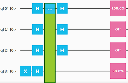
Similar to the Deutsch algorithm, when f(x) is a constant function, this equation shows that the probability of measuring 0 on the first qubit is 100%. When f(x) is a balanced function, the first qubit will always be measured as 1 (as the probability of measuring 0 is null).
The code in the example randomly picks one of two predefined oracles. The first oracle corresponds to the Identity gate, and that corresponds to a constant function that always returns 0. The second oracle corresponds to a CNot gate, where the ancilla qubit is swapped when the last input qubit is 1.
Again, our goal is not to create those oracles. You can assume that the oracles are somehow provided to you, and you have to find out if they correspond to either constant or balanced functions.
9.8 Conclusion
In this chapter, you created the Deutsch-Jozsa algorithm. While there is no direct practical usage of this algorithm, you achieved a major milestone. For the first time in this book, you created a quantum algorithm that can execute a task much faster than a corresponding classical algorithm. The real speedup can only be seen if you use a real quantum computer; but the algorithms you created clearly show that a single evaluation is required to fix a specific problem, whereas in classical computing an exponential number of evaluations is required.
Two very important but challenging parts of quantum computing are
-
Coming up with quantum algorithms like this that are proven to be faster than corresponding classical algorithms
In the next chapters, we discuss two algorithms that satisfy these requirements.
Summary
-
Some problems can be solved without calculating the end results.
-
There is a difference between function evaluation and function properties.
-
Classical algorithms can distinguish between balanced and constant functions, but they require many function evaluations to do so.
-
A quantum oracle is a black box related to a classical black box function.
-
Using the Deutsch-Jozsa algorithm, you can detect whether a supplied oracle corresponds to a balanced or constant function.