
11
Entanglement Measures
Martin B. Plenio1 and Shashank S. Virmani2
1 Universität Ulm, Institute of Theoretical Physics, Albert‐Einstein‐Allee 11, 89081 Ulm, Germany
2 Brunel University London, College of Engineering, Design and Physical Sciences, Kingston Lane, Uxbridge, Middlesex UB8 3PH, United Kingdom
11.1 Introduction
The concept of entanglement has played an important role in quantum physics ever since its discovery last century and has now been recognized as a key resource in quantum information science (1–5). However, despite its evident importance, entanglement remains an enigmatic phenomenon. One important avenue to understand this enigma is via the study of entanglement measures. In this chapter, we will discuss the motivation behind this approach, and present the implications of entanglement measures for the study of entanglement in quantum information science. Space limitations mean that there are several interesting results that we will not be able to treat in sufficient detail or that we cannot mention at all. However, we hope that this chapter will give the reader a first glimpse on the subject and will enable them to independently tackle the extensive literature on this topic. Many more details can be found in various review articles (1–6). The majority of this chapter will concentrate on entanglement in bipartite systems, for which the most complete understanding has been obtained so far, and we will only indicate how to approach the multiparty setting. For a more careful discussion of the multiparty setting, we refer the reader to Chapter 13. We will not be able at all to touch upon the study of entanglement in interacting many‐body systems, which has become an area of active research recently (see, e.g., (7–14)).
Any study of entanglement measures must begin with a discussion of what entanglement is, and how we actually use it. The term entanglement has become synonymous with highly nonclassical tasks such as violating locality (15), teleportation (16), and dense coding (17), and so for an initial definition, we may vaguely say that entanglement is “that property of quantum states that enables these feats.” To flesh out this definition properly, we need to consider how we will actually use this entanglement. A typical quantum communication situation in which we use entanglement is as follows: we assume that two distantly separated parties (the proverbial “Alice” and “Bob”) have access to one particle each from a joint quantum state. In addition, we assume that they have the ability to communicate classically and perform arbitrary local operations on their individual particles. These restrictions form the paradigm of Local Operations and Classical Communication , or LOCC for short. We allow Alice and Bob to communicate classically for two important reasons. Firstly, classical communication can be used to establish classical correlations between sender and receiver. As a consequence, the additional power provided by entanglement can then be expected to be due to quantum correlations. Secondly, from a practical point of view, classical communication is also technologically simple, which justifies its addition to the set of essentially free resources.
So, given that we can exploit entangled quantum states using LOCC operations, what are the properties of entangled quantum states that make them so “useful” for the “nonclassical” tasks of quantum information? Unfortunately, this question is too simplistic to have a rigorous answer. There is a vast diversity of such “nonclassical” tasks, and just because a state has properties that are “useful” for one task does not mean that it is useful for another. However, despite this variety, it is possible to make a few important remarks that apply generally:
-
Separable states contain no entanglement. A state ρ
ABC… of many parties A, B, C, … is said to be separable (18), if it can be written in the formwhere pi is a probability distribution. These states can trivially be created by LOCC–Alice samples from the distribution pi , tells all other parties the outcome, and then each party X locally creates
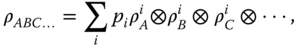
 . As these states can be created from scratch by LOCC, they trivially satisfy a local hidden variables' model, and do not allow us to perform teleportation (1) better than we could using LOCC only. Hence, separable states can be said to contain no entanglement and LOCC cannot create entanglement from an unentangled state. Indeed, we even have the following stronger fact.
 - The entanglement of states decreases under LOCC transformations. Suppose that we know that a certain quantum state ρ can be transformed to another quantum state σ using LOCC operations. Then anything that we can do with σ we can also do with ρ. Hence, the utility of quantum states can only decrease under LOCC operations (1 19–21), and one can say that ρ is more entangled than σ. Note that this definition of “entangled” is implicitly related to the assumption of LOCC restrictions – if other restrictions apply, weaker or stronger, then our notion of “more entangled” is also likely to change.
- Entanglement does not change under local unitary operations. This is because local unitaries can be inverted by local unitaries. Hence, by the nonincrease of entanglement under LOCC, two states related by local unitaries have equivalent entanglement.
-
In two party systems consisting of two d‐dimensional systems, the pure states local unitarily equivalent to
 are maximally entangled. This is well justified, because as we shall see later, any pure or mixed state of two d‐dimensional systems can be reached from such states using only LOCC operations.
The above considerations have given us the extremes of Entanglement – as long as we consider LOCC as our definitive set of operations, separable states contain zero entanglement, and we can identify certain states that have maximal entanglement. They also suggest that we can impose some form of ordering – we may say that state ρ is more entangled than a state σ if we can perform the transformation ρ → σ using LOCC operations. A key question is whether this method of ordering gives a partial or total order? To answer this question, we must try and find out when one quantum state may be transformed to another using LOCC operations. We will consider this question in more detail in the next part, where we will find that in general LOCC ordering only results in a partial order.
This means that in general an LOCC‐based classification of entanglement is extremely complicated. However, one can obtain a more digestible classification by making extra demands on our definition of entanglement. By adding extra ingredients, one can obtain real‐valued functions that attempt to quantify the amount of entanglement in a given quantum state. This is essentially the process that is followed in the definition of entanglement measures. Various entanglement measures have been proposed over the years, such as the entanglement of distillation (19,22), the entanglement cost (19 23–25), the relative entropy of entanglement (20,21,26), and the squashed entanglement (27). Some of these have direct physical significance, whereas others are axiomatic quantities. The initial advantage of these measures was that they gave a physically motivated classification of entanglement that is simple to understand. However, they have also developed into powerful mathematical tools, with major significance for open questions such as the additivity of channel capacities (28,29). We will return to the development of entanglement measures later, but we must first understand in more detail some essential aspects of the manipulation of quantum states under LOCC.
11.2 Manipulation of Single Systems
In the previous section, we had indicated that for bipartite systems there is a notion of maximally entangled states that is independent of the specific quantification of entanglement. This is so, because there are states from which all others can be created by LOCC only. We consider here the case of two two‐level systems and leave the generalization as an exercise to the reader. The maximally entangled states then take the form
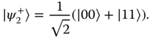
Our aim is now to justify this statement by showing that for any pure state
we can find a LOCC map that takes ![]() to |φ〉 with certainty. To this end, we simply need to write the Kraus operators of a valid operation. Clearly,
to |φ〉 with certainty. To this end, we simply need to write the Kraus operators of a valid operation. Clearly,
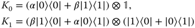
satisfies ![]() and Ki
|ψ〉 ∼ |φ〉. It is a worthwhile exercise to try and construct this operation by adding ancillas to the systems, carrying out local unitary operations, followed by projective measurements and classical communication. Given that we can obtain with certainty any arbitrary pure state starting from
and Ki
|ψ〉 ∼ |φ〉. It is a worthwhile exercise to try and construct this operation by adding ancillas to the systems, carrying out local unitary operations, followed by projective measurements and classical communication. Given that we can obtain with certainty any arbitrary pure state starting from ![]() we can also obtain any mixed state ρ. This is because
we can also obtain any mixed state ρ. This is because ![]() where |φi
〉 = Ui
⊗ Vi
(αi
|00〉 + βi
|11〉) with unitaries Ui
and Vi
. It is an easy exercise, left to the reader, to construct the operation that takes
where |φi
〉 = Ui
⊗ Vi
(αi
|00〉 + βi
|11〉) with unitaries Ui
and Vi
. It is an easy exercise, left to the reader, to construct the operation that takes ![]() to ρ.
to ρ.
A natural next question to consider is the LOCC transformation between general pure states of two parties (30). Indeed, a mathematical framework based on the theory of majorization has been developed that provides necessary and sufficient conditions for the interconversion between two pure states, together with protocols that achieve the task (31–33). Let us write the initial and final state vectors as |ψ 1〉 and |ψ 2〉 in their Schmidt basis,
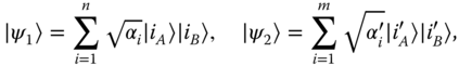
where n denotes the dimension of each of the quantum systems. We can take the Schmidt coefficients to be given in decreasing order, that is, α
1 ≥ α
2 ≥⋯≥ αn
and ![]() ≥⋯≥
≥⋯≥ ![]() . The question of the interconvertability between the states can then be decided from the knowledge of the real Schmidt coefficients only. One finds that a LOCC transformation that converts |ψ
1〉 to |ψ
2〉 with unit probability exists if and only if the {αi
} are majorized (34) by {
. The question of the interconvertability between the states can then be decided from the knowledge of the real Schmidt coefficients only. One finds that a LOCC transformation that converts |ψ
1〉 to |ψ
2〉 with unit probability exists if and only if the {αi
} are majorized (34) by {![]() }, that is, exactly if for all 1 ≤ l ≤ n
}, that is, exactly if for all 1 ≤ l ≤ n
Various refinements of this result have been found that provide the largest success probabilities for the interconversion between two states by LOCC together with the optimal protocol where a deterministic interconversion is not possible (32,33). These results allow in principle to decide any question concerning the LOCC interconversion of pure state by employing techniques from linear programming (33). Although the basic mathematical structure is well understood, surprising and not yet fully understood effects such as entanglement catalysis are still possible (35). It is a direct consequence of the above structures that there are incomparable states, that is, pairs of states such that neither can be converted into the other with certainty. These states are called incomparable as neither can be viewed as more entangled than the other. The following part will serve to overcome this problem for pure states.
11.3 Manipulation in the Asymptotic Limit
The study of the LOCC transformation of pure states so far has enabled us to justify the concept of maximally entangled states and also permitted, in some cases, to assert that one state is more entangled than another. However, we know that exact LOCC transformations can only induce a partial order on the set of quantum states. The situation is even more complex for mixed states, where even the question of the transformation from one state into another by LOCC is a difficult problem with no transparent solution.
All this means that if we want to give a definite answer as to whether one state is more entangled than another for any pair of states, it will be necessary to consider a more general setting. In this context, a very natural way to quantify entanglement is to study LOCC transformations of states in the so‐called asymptotic regime. Instead of asking whether a single initial state ρ may be transformed to a final state σ by LOCC operations, we may ask whether for some large integers m, n, we can implement the “wholesale” transformation ρ ⊗n → σ ⊗m to a high level of approximation. In a loose sense, that will be made more rigorous later, we may use the optimal possible rate of transformation m/n as a measure of how much more (or less) entanglement ρ has as compared to σ. This asymptotic setting may be viewed as a limiting case of the above theorems for arbitrarily high dimensions, and indeed predated it (19). It turns out that in the pure state case the study of the asymptotic regime gives a very natural measure of entanglement that is essentially unique.
To understand the asymptotic regime precisely, we first need to understand the issue of approximation. In principle, we could ask what the optimal rate of conversion m/n is for exact transformations of the form ρ ⊗n → σ ⊗m . However, from the theorems of the previous section we know that exact pure state transformations are not always possible with LOCC. Therefore, the fact that there are incomparable pure states means that we will not be able to use asymptotic conversion rates to quantify entanglement for all states unless we admit some form of imperfection. One way to admit such imperfections is to allow transformations such that for finite n the output only approximates the target according to a suitably chosen distance measure, such that these imperfections vanish in the limit n → ∞. From a physical point of view allowing such approximate transformations is quite acceptable, as vanishingly small imperfections will not affect observations of the output in any perceptible way.
Let us formalize these notions for one of the most important entanglement measures, the entanglement cost, EC
(ρ). For a given state ρ, this measure quantifies the maximal possible rate at which one can convert input maximally entangled states of two qubits into output states that approximate ρ. If we denote a general trace preserving LOCC operation by Ψ, and write Φ(K) for the density operator corresponding to the maximally entangled state vector in K dimensions, that is, Φ(K) = ![]() , then the entanglement cost may be defined as
, then the entanglement cost may be defined as
where D(x, y) is a suitable measure of distance. A variety of possible distance measures may be proposed, but two natural choices are the trace distance or the Bures distance (34,36), as these functions can be used to bound the statistical differences between two states. It has been shown that the definition of entanglement cost is independent of the choice of distance function, as long as these functions are equivalent in a way that is independent of dimension (see (25) for further explanation), and so we will fix the trace norm as our choice for D(x, y).
The entanglement cost is an important measure because it quantifies a wholesale “exchange rate” for converting from maximally entangled states to copies of ρ, and maximally entangled states are in essence the “gold standard currency” with which one would like to compare all quantum states. Although computing EC (ρ) is extremely difficult, we will later discuss its important implications for the study of channel capacities, in particular via another important entanglement measure known as the entanglement of formation, EF (ρ).
In addition to the entanglement cost, another important asymptotic entanglement measure is the distillable entanglement, D(ρ), which is a kind of dual measure to the entanglement cost. Just as EC (ρ) measures how many maximally entangled states are required to create copies of ρ, we can ask about the reverse process: at what rate may we obtain maximally entangled states (of two qubits) from an input supply of ρ. This process is known in the literature either as entanglement distillation, or as entanglement concentration. Again we allow the output of the procedure to approximate many copies of a maximally entangled state, as the exact transformation from ρ ⊗n to even one singlet state is in general impossible (37). In analogy to the definition of EC (ρ), we can make the precise mathematical definition of D(ρ) as
D(ρ) is an important measure because if entanglement is required in a two party quantum information protocols, then it is usually required in the form of maximally entangled states. So D(ρ) tells us the rate at which noisy mixed states may be converted back into the “gold standard” singlet states. In defining D(ρ) we have overlooked a couple of important issues. Firstly, our LOCC protocols are always taken to be trace preserving. However, one could conceivably allow probabilistic protocols that have varying degrees of success depending upon various measurement outcomes. Fortunately, a thorough paper by Rains (22) shows that taking into account a wide diversity of possible success measures still leads to the same notion of distillable entanglement. Secondly, we have always used two qubits maximally entangled states as our “gold standard,” if we use other entangled pure states, perhaps even on higher dimensions, do we arrive at significantly altered definitions? We will very shortly see that this is not the case, and there is no loss of generality in taking singlet states as our target.
A remarkable feature of the asymptotic transformations regime is that pure state transformations become reversible. Indeed, for pure states it turns out that both D(ρ) and EC (ρ) are identical and equal to the entropy of entanglement (19), which for a pure state |ψ〉 is defined as
where S denotes the von‐Neumann entropy S(ρ) = −tr[ρ log2 ρ], and tr B denotes the partial trace over subsystem B. This reversibility means that in the asymptotic regime we may immediately write the optimal rate of transformation between any two pure states |ψ 1〉 and |ψ 2〉. Given a large number N of copies of |ψ 1〉〈ψ 1|, we can first distill ≈ NE(|ψ 1〉〈ψ 1|) singlet states and then create from those singlets M ≈ NE(|ψ 1〉〈ψ 1|)/E(|ψ 2〉〈ψ 2|) copies of |ψ 2〉〈ψ 2|. In the infinite limit these approximations become exact, and as a consequence E(|ψ 1〉〈ψ 1|)/E(|ψ 2〉〈ψ 2|) is the optimal asymptotic conversion rate from |ψ 1〉〈ψ 1| to |ψ 2〉〈ψ 2|. It is the reversibility of pure state transformations that enables us to define D(ρ) and EC (ρ) in terms of transformations to or from singlet states – use of any other entangled state (in any other dimensions) simply leads to a constant factor multiplied in front of these quantities.
Following these basic considerations, we are now in a position to formulate a more rigorous and axiomatic approach to entanglement measures that try to capture the lessons that have been learned in the previous sections. In the final section, we will then review several entanglement measures and discuss their significance for various topics in quantum information.
11.4 Postulates for Axiomatic Entanglement Measures: Uniqueness and Extremality Theorems
In the previous section, we considered the quantification of entanglement from the perspective of LOCC transformations in the asymptotic limit. This approach is interesting because it can be solved completely for pure states, and leads to two of the most important entanglement measures for mixed states – the distillable entanglement and entanglement cost. However, computing these measures is extremely difficult for mixed states, and so in this section we will discuss a more axiomatic approach to quantifying entanglement. This approach has proven very fruitful: among other applications axiomatic entanglement measures have been used to assess the quality of entangled states produced in experiments, to understand the behavior of correlations during quantum phase transitions, to bound fault tolerance thresholds in quantum computation, and derive several interesting results in the study of channel capacities.
So what exactly are the properties that a good entanglement measure should possess? An entanglement measure is a mathematical quantity that should capture the essential features that we associate with entanglement, and ideally should be related to some operational procedure. Depending upon your aims, this can lead to variety of possible desirable properties. The following is a list of possible postulates for entanglement measures, some of which are not satisfied by all proposed quantities (21,38):
- A bipartite entanglement measure E(ρ) is a mapping:defined for states of arbitrary bipartite systems. A normalization factor is also usually included such that the singlet state
 of two qubits has
  .
. - E(ρ) = 0 if the state ρ is separable.
-
E does not increase on average under LOCC, that is,where in a LOCC protocol applied to state ρ the state ρi with label i is obtained with probability pi .
- For pure state |ψ〉〈ψ| the measure reduces to the entropy of entanglement

We will call any function E satisfying the first three conditions an entanglement monotone, usually reserving the term entanglement measure only for quantities satisfying the fourth condition. In the literature, these terms are often used interchangeably. Frequently, some authors also impose additional requirements for entanglement measures. One common example is requiring convexity, that is, E(∑ ipiρi ) ≤ ∑ ipiE(ρi ). This mathematically very convenient property is sometimes justified as capturing the notion of the loss of information, that is, describing the process of going from a selection of identifiable states ρi that appear with rates pi to a mixture of these states of the form ρ = ∑piρi . We would like to stress, however, that this particular requirement is not essential. Indeed, in the first situation, before the loss of information about the state, the whole ensemble can be described by the single quantum state
where {|i〉
M
} denote some orthonormal basis belonging to one party. Clearly a measurement of the marker particle M reveals the identity of the state of parties A and B. The process of the forgetting is then described by tracing out the marker particle M to obtain ρ = ∑piρi
(39). Therefore, we can require that E(∑
ipi
|i〉
M
〈i| ⊗ ![]() ) ≥ E(ρ), which is already captured by condition 3 above. Hence, there is no need to require convexity, except for the mathematical simplicity that it might bring.
) ≥ E(ρ), which is already captured by condition 3 above. Hence, there is no need to require convexity, except for the mathematical simplicity that it might bring.
The first three conditions listed above seem quite natural – the first two conditions are little more than setting the scale, and the third condition is a generalization of the idea that entanglement can only decrease under LOCC operations to incorporate probabilistic transformations. The fourth condition may seem a little strong. However, it turns out that it is also quite a natural condition to impose. The fact that S(ρA
) represents the reversible rate of conversion between pure states in the asymptotic regime actually forces any entanglement monotone that is (a) additive on pure states, and (b) sufficiently continuous, to be equal to S(ρA
) on the pure states. A very rough argument is as follows. We know from the asymptotic pure state distillation protocol that from n copies of a pure state |φ〉 we can obtain a state ρn
that closely approximates the state ![]() ⊗nE(|φ〉) to within ε, where E(|φ〉) is the entropy of entanglement of |φ〉. Suppose that we have an entanglement monotone L that is additive on pure states. Then we may write
⊗nE(|φ〉) to within ε, where E(|φ〉) is the entropy of entanglement of |φ〉. Suppose that we have an entanglement monotone L that is additive on pure states. Then we may write
If the monotone L is sufficiently continuous, then L(ρn
) = L(![]() ⊗nE(|φ〉)) + δ(ε) = nE(|φ〉) + δ(ε), where δ(ε) will be small. Then we obtain
⊗nE(|φ〉)) + δ(ε) = nE(|φ〉) + δ(ε), where δ(ε) will be small. Then we obtain
If the function L is remains sufficiently continuous as the dimension increases then δ(ε)/n → 0, and we obtain L(|φ〉) ≥ E(|φ〉). We will see a little later exactly what sufficiently continuous means. Invoking the fact that the entanglement cost for pure states is also given by the entropy of entanglement gives the reverse inequality L(|φ〉) ≤ E(|φ〉) using similar arguments. Hence sufficiently continuous monotones that are additive on pure states will naturally satisfy L(|φ〉) = E(|φ〉). Of course these arguments are not rigorous, as we have not undertaken a detailed analysis of how δ or ε grow with n. A rigorous analysis is presented in (38), where it is also shown that our assumptions may be slightly relaxed. The result of this rigorous analysis is that a function is equivalent to the entropy of entanglement on pure states if and only if it is (a) normalized on the singlet state, (b) additive on pure states, (c) nonincreasing on deterministic pure state to pure state LOCC transformations, and (d) asymptotically continuous on pure states. The term asymptotically continuous is defined as the property
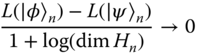
whenever the trace norm ![]() between two sequences of states |φ〉
n
, |ψ〉
n
on a sequence of Hilbert spaces Hn
⊗ Hn
tends to 0 as n → 0. It is interesting to note that these constraints only concern pure state properties of L, and that they are necessary and sufficient. It is interesting to note that any monotones that satisfy (a)–(d) cannot have qualitative agreement with each other, that is, imposing the same order on states, unless they are exactly the same (40) (see (41) for ordering results for other entanglement quantities).
between two sequences of states |φ〉
n
, |ψ〉
n
on a sequence of Hilbert spaces Hn
⊗ Hn
tends to 0 as n → 0. It is interesting to note that these constraints only concern pure state properties of L, and that they are necessary and sufficient. It is interesting to note that any monotones that satisfy (a)–(d) cannot have qualitative agreement with each other, that is, imposing the same order on states, unless they are exactly the same (40) (see (41) for ordering results for other entanglement quantities).
In addition to the above uniqueness theorem, it turns out that similar arguments may be used to show that the entanglement cost EC (ρ) and the distillable entanglement D(ρ) are in some sense extremal measures (38,42), in that they are upper and lower bounds for many “wholesale” entanglement monotones. To be precise, suppose that we have a quantity L(ρ) satisfying conditions (1)–(3), that is also asymptotically continuous on mixed states, and also has a regularization:
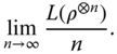
Then it can be shown that
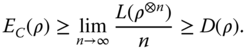
Equations such as these may be useful for deriving upper bounds on D(ρ). However, the resulting bounds may be very difficult to calculate if the entanglement measures involved are defined as variational quantities. In this context, it is important to mention a quantity known as the conditional entropy, which is defined as C(A|B): = S(ρAB ) − S(ρB ) for a bipartite state ρAB . It was known for some time that −C(A|B) gives a lower bound for both the entanglement cost and another important measure known as the relative entropy of entanglement (43). This bound was also recently shown to be true for the one way distillable entanglement:
where D A→B is the distillable entanglement under the restriction that the classical communication may only go one way from Alice to Bob (44). This bound is known as the Hashing inequality, and is significant as it is a computable, nontrivial, lower bound to D(ρ), and hence supplies a nontrivial lower bound to many other entanglement measures.
11.5 Examples of Axiomatic Entanglement Measures
In this section, we discuss a variety of the bipartite axiomatic entanglement measures that have been proposed in the literature. All the following quantities are entanglement monotones, in that they cannot increase under LOCC, and hence when they can be calculated, can be used to determine whether certain LOCC transformations are possible, often both in the finite and asymptotic regimes. However, some measures have a wider significance, that we will discuss as they are introduced. Note that the list of entanglement measures mentioned here is only a subset of many proposals. We have selected this list of measures on the basis of those with which we are most familiar, and there are many other important approaches that we are not able to discuss in detail.
-
Entanglement of formation. For a mixed state ρ, this measure is defined as
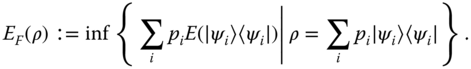
The heuristic motivation for this measure is that it is the minimal possible average entanglement over all pure state decompositions of ρ, where ![]() is taken as the measure of entanglement for pure states. The variational problem that defines EF
is extremely difficult to solve. However, closed solutions are known for two‐qubit states, and for certain cases of symmetry (24). The regularized or asymptotic version of the entanglement of formation is defined as
is taken as the measure of entanglement for pure states. The variational problem that defines EF
is extremely difficult to solve. However, closed solutions are known for two‐qubit states, and for certain cases of symmetry (24). The regularized or asymptotic version of the entanglement of formation is defined as ![]() . The regularized version is important as it can be rigorously shown to be equal to the entanglement cost (25)
. The regularized version is important as it can be rigorously shown to be equal to the entanglement cost (25)
A major open question in quantum information is to decide whether EF is an additive quantity, that is,
This problem is known to be equivalent to the strong superadditivity of EF
The major importance of these additivity problems stems not only from the fact that they would show that EF = EC , but also because they are equivalent to both the additivity of the minimal output entropy of quantum channels, and the additivity of the classical communication capacity of quantum channels!
EF is an important example of a convex roof construction. The convex roof of a function f that is defined on the extremal points of a convex set is the largest convex function that matches f on the extreme points. It is easy to see that EF is the convex roof of the entropy of entanglement, and is hence the largest of all convex functions that agree with S(ρA ) on the pure states. The convex roof method can be used to construct entanglement monotones from any unitarily invariant (including isometric embeddings) concave function of density matrices (45).
-
Relative entropy of entanglement (20,21,43). An intuitive way of constructing an entanglement measure is to quantify how difficult it is to discriminate an entangled state from a set X of disentangled states. The relative entropy is one way of quantifying this. For two quantum states ρ, σ it is defined as

So a natural entanglement measure, dependent upon the choice of X, is
This definition leads to a class of entanglement measures known as the relative entropies of entanglement. In the bipartite setting, the set X can be taken as the set of separable, PPT, or nondistillable states, depending upon your favorite definition of disentangled. In the multiparty setting, there are even more possibilities (46,47). In the bipartite setting, the measures ![]() are equal to the entropy of entanglement for bipartite pure states. The bipartite relative entropies have been used to compute tight upper bounds to the distillable entanglement of certain states, and as an invariant to help decide the asymptotic interconvertibility of multipartite states.
are equal to the entropy of entanglement for bipartite pure states. The bipartite relative entropies have been used to compute tight upper bounds to the distillable entanglement of certain states, and as an invariant to help decide the asymptotic interconvertibility of multipartite states.
The relative entropy measures are known in general not to be additive, as bipartite states can be found where
In some such cases, the regularized versions of some relative entropy measures can be calculated (48,49).
The relative entropy functional is only one possible “distinguishability measure” between states, and in principle one could use other distance functions to quantify how far a particular state is from a chosen set of disentangled states. Many interesting examples of other functions that can be used for this purpose may be found in the literature (see, e.g., (20,50)). It is also worth noting that the relative entropy functional is asymmetric, in that S(ρ|σ) ≠ S(σ|ρ). This is connected with asymmetries that can occur in the discrimination of probability distributions (21). One can consider reversing the arguments and tentatively define an LOCC monotone JX (ρ) ≔ inf{S(σ|ρ) |σ ∈ X}. The resulting function has the advantage of being additive, but unfortunately it has the problem that it can be infinite on pure states (51).
-
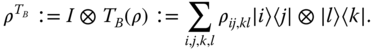
Logarithm of the negativity. The partial transposition with respect to party B of a bipartite state ρAB
expanded in given local orthonormal basis as ρ = ρ
ij,kl
|i〉〈j| ⊗ |k〉〈l| is defined as
The spectrum of the partial transposition of a density matrix is independent of the choice of local basis, and is independent of whether the partial transposition is taken over party A or party B. The positivity of the partial transpose of a state is a necessary condition for separability (52), and is sufficient to prove that D(ρ) = 0 for a given state. The quantity known as the Negativity (41,53), N(ρ), is an entanglement monotone (54,55) that attempts to quantify the negativity in the spectrum of the partial transpose. We will define the Negativity as
where ![]() is the trace norm. Note that many authors define the Negativity differently as
is the trace norm. Note that many authors define the Negativity differently as ![]() . With the convention that we follow, the Logarithm of the Negativity is defined as
. With the convention that we follow, the Logarithm of the Negativity is defined as
EN is an entanglement monotone that cannot increase under deterministic LOCC operations, as well as on average under probabilistic LOCC transformations. It is additive by construction, and convex due to its monotonic relationship to a norm. Although EN is manifestly continuous, it is not asymptotically continuous, and hence does not reduce to the entropy of entanglement on all pure states. Later we will see that N(ρ) is part of a larger family of monotones that be constructed in a similar way.
The major practical advantage of EN is that it can be calculated very easily; however, it also has various operational interpretations as an upper bound to D(ρ), a bound on teleportation capacity (55), and an asymptotic entanglement cost under the set of PPT operations (56).
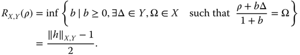
EN can also been combined with a relative entropy approach to give another monotone known as the Rains' Bound (57), which is defined as:
One can see that almost by definition B(ρ) is a lower bound to ![]() , and it can also be shown that it is an upper bound to the distillable entanglement. It is interesting to observe that for Werner states B(ρ) happens to be equal to
, and it can also be shown that it is an upper bound to the distillable entanglement. It is interesting to observe that for Werner states B(ρ) happens to be equal to ![]() (48,57), a connection that has been explored in more detail in (49,56,58).
(48,57), a connection that has been explored in more detail in (49,56,58).
-
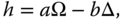
Norm‐based monotones. In (55) it was noted that the Negativity described above is part of a general family of entanglement monotones (related to an even wider concept known as a base norm). To construct this family, we require two sets X, Y of Hermitian matrices satisfying the following conditions: (a) X, Y are closed under LOCC operations (even measuring ones), (b) X, Y are convex cones (i.e., also closed under multiplication by nonnegative scalars), and (c) any Hermitian operator h may be expanded aswhere Ω ∈ X, Δ ∈ Y are normalized (i.e., trace 1) but not necessarily positive, and a, b ≥ 0. Given two such sets X, Y and any Hermitian operator h we may define
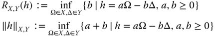
Note that for when ρ is a state (i.e., positive, trace 1), the first of these functions R X, Y may be rewritten as
From this equation, we see if Ω, Δ are also states, then R X,Y , which is monotonically related to R X,Y /(1 + R X,Y ), quantifies the minimal noise of type Y that must be mixed with ρ to give a state of the form X. For this reason, we will refer to quantities of the type of R X,Y (ρ) as robustness monotones. It can be shown that the restrictions on X, Y force R X,Y (ρ) to be convex, ‖h‖ X,Y to be a norm, and both quantities to be LOCC monotones.
Examples of robustness monotones are the “robustness,” where both X, Y are the set of separable states, and the “global robustness,” where X is the set of separable states and Y is the set of all states (59,60) (note that the “random robustness” is not a monotone, for definition and proof see (59)). These monotones can often be calculated or at least bounded nontrivially, and have found applications in areas such as bounding fault tolerance (59,60). The Negativity introduced above also fits into this class of monotones – it is simply ‖ρ‖ X,Y where both X, Y are the set of normalized Hermitian matrices with positive partial transposition.
Another form of norm‐based entanglement monotone is the cross norm monotone proposed in (61). The greatest cross norm of an operator A is defined as
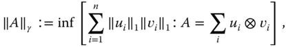
where ‖y‖1: = ![]() is the trace norm, and the infimum is taken over all decompositions of A into finite sums of product operators. It can be shown that a density matrix ρAB
is separable iff ‖ρ‖
γ
= 1, and that the quantity
is the trace norm, and the infimum is taken over all decompositions of A into finite sums of product operators. It can be shown that a density matrix ρAB
is separable iff ‖ρ‖
γ
= 1, and that the quantity
is an entanglement monotone (61). As it is expressed as a complicated variational expression, Eγ (ρ) can be difficult to calculate. However, for pure states and cases of high symmetry it may often be computed exactly. Although Eγ (ρ) does not fit precisely into the family of base norm monotones discussed above, there is a relationship. If the sum in 10.1 is restricted to Hermitian ui and vi , then we recover precisely the base norm ‖A‖ X,Y , where X, Y are taken as the set of separable states. Hence, Eγ is an upper bound to the robustness (61).
-
Squashed entanglement. The “squashed” entanglement (27) (see also (62)) is a recently proposed measure that is defined as
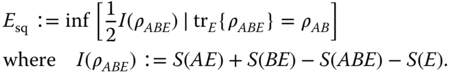
In this definition, I(ρABE ) is the quantum conditional mutual information, which is often also denoted as I(A; B|E). The squashed entanglement is a convex entanglement monotone that is a lower bound to EF (ρ) and an upper bound to D(ρ), and is hence automatically equal to S(ρA ) on pure states. It is also additive on tensor products, and is hence a useful nontrivial lower bound to EC (ρ). The intuition behind E sq is that it “squashes out” the classical correlations between Alice, Bob, and the third party Eve, an idea motivated by related quantities in classical cryptography.
Acknowledgments
This work is part of the QIP‐IRC (www.qipirc.org) supported by EPSRC (GR/S82176/0) as well as the EU (IST‐2001‐38877) the Leverhulme Trust, and the Royal Commission for the Exhibition of 1851.
References
- 1 Plenio, M.B. and Vedral, V. (1998) Contemp. Phys., 39, 431.
- 2 Schumacher, B. (2002) Relative entropy in quantum information theory, in Quantum Computation and Information (eds S.J. Lomonaco, Jr. and H.E. Brandt), vol. 305 of “Contemporary Mathematics”, American Mathematical Society, Providence, RI, pp. 265–290.
- 3 Horodecki, M. (2001) Quant. Inf. Comp., 1, 3.
- 4 Horodecki, P. and Horodecki, R. (2001) Quant. Inf. Comp., 1, 45.
- 5 Eisert, J. and Plenio, M.B. (2003) Int. J. Quant. Inf., 1, 479.
- 6 Plenio, M.B. and Virmani, S. (2007) Quantum Inf. Comput., 7, 1.
- 7 Audenaert, K., Eisert, J., Plenio, M.B., and Werner, R.F. (2002) Phys. Rev. A, 66, 042327.
- 8 Botero, A. and Reznik, B. (2004) Phys. Rev. A, 70, 052329.
- 9 Carteret, H., Preprint quant‐ph/0405168.
- 10 Eisert, J., Plenio, M.B., Bose, S., and Hartley, J. (2004) Phys. Rev. Lett., 93, 190402.
- 11 Verstraete, F., Martin‐Delgado, M.‐A., and Cirac, J.I. (2004) Phys. Rev. Lett., 92, 087201.
- 12 Pachos, J.K. and Plenio, M.B. (2004) Phys. Rev. Lett., 93, 056402.
- 13 Plenio, M.B., Eisert, J., Dreißig, J., and Cramer, M. (2005) Phys. Rev. Lett., 94, 060503.
- 14 Cramer, M., Eisert, J., Plenio, M.B., and Dreißg, J. (2006) Phys. Rev. A, 73, 012309.
- 15 Bell, J.S. (1964) Physics, 1, 195.
- 16 Bennett, C.H., Brassard, G., Crepeau, C., Jozsa, R., Peres, A., and Wootters, W.K. (1993) Phys. Rev. Lett., 70, 1895.
- 17 Bennett, C.H. and Wiesner, S. (1992) Phys. Rev. Lett., 69, 2881.
- 18 Werner, R.F. (1989) Phys. Rev. A, 40, 4277.
- 19 Bennett, C.H., Bernstein, H., Popescu, S., and Schumacher, B. (1996) Phys. Rev. A, 53, 2046.
- 20 Vedral, V., Plenio, M.B., Rippin, M.A., and Knight, P.L. (1997) Phys. Rev. Lett., 78, 2275.
- 21 Vedral, V. and Plenio, M.B. (1998) Phys. Rev. A, 57, 1619.
- 22 (a) Rains, E. (1999) Phys. Rev. A, 60, 173; (b) Rains, E. (1999) Phys. Rev. A, 60, 179.
- 23 Bennett, C.H., DiVincenzo, D.P., Smolin, J.A., and Wootters, W.K. (1996) Phys. Rev. A, 54, 3824.
- 24 Wootters, W.K. (1998) Phys. Rev. Lett., 80, 2245.
- 25 Hayden, P., Horodecki, M., and Terhal, B.M. (2001) J. Phys. A: Math. Gen., 34, 6891.
- 26 Vollbrecht, K.G.H. and Werner, R.F. (2001) Phys. Rev. A, 64, 062307.
- 27 Christandl, M. and Winter, A. (2004) J. Math. Phys., 45, 829.
- 28 Shor, P.W. (2004) Commun. Math. Phys., 246, 453.
- 29 Audenaert, K.M.R. and Braunstein, S.L. (2003) Commun. Math. Phys., 246, 443.
- 30 Lo, H.‐K. and Popescu, S. (2001) Phys. Rev. A, 63, 022301.
- 31 Nielsen, M.A. (1999) Phys. Rev. Lett., 83, 436.
- 32 Vidal, G. (1999) Phys. Rev. Lett., 83, 1046.
- 33 Jonathan, D. and Plenio, M.B. (1999) Phys. Rev. Lett., 83, 1455.
- 34 Bhatia, R. (1997) Matrix Analysis, Springer, Berlin.
- 35 Jonathan, D. and Plenio, M.B. (1999) Phys. Rev. Lett., 83, 3566.
- 36 Nielsen, M. and Chuang, I. (2000) Quantum Information and Computation, Cambridge University Press, Cambridge, MA.
- 37 Kent, A. (1998) Phys. Rev. Lett., 81, 2839.
- 38 Donald, M.J., Horodecki, M., and Rudolph, O. (2002) J. Math. Phys., 43, 4252.
- 39 Plenio, M.B. and Vitelli, V. (2001) Contemp. Phys., 42, 25.
- 40 Virmani, S. and Plenio, M.B. (2000) Phys. Lett. A, 288, 62.
- 41 (a) Eisert, J. and Plenio, M.B. (1999) J. Mod. Opt., 46, 145; (b) Zyczkowski, K. and Bengtsson, I. (2002) Ann. Phys., 295, 115; (c) Miranowicz, A. and Grudka, A. (2004) J. Opt. B: Quantum Semiclass. Opt., 6, 542–548.
- 42 Horodecki, M., Horodecki, P., and Horodecki, R. (2000) Phys. Rev. Lett., 84, 2014.
- 43 Plenio, M.B., Virmani, S., and Papadopoulos, P. (2000) J. Phys. A: Math. Gen., 33, L193.
- 44 Devetak, I. and Winter, A. (2005) Proc. R. Soc. Lond. A, 461, 207.
- 45 Vidal, G. (2000) J. Mod. Opt., 47, 355.
- 46 Plenio, M.B. and Vedral, V. (2001) J. Phys. A: Math. Gen., 34, 6997.
- 47 Vedral, V., Plenio, M.B., Jacobs, K., and Knight, P.L. (1997) Phys. Rev. A, 56, 4452.
- 48 Audenaert, K., Eisert, J., Jané, E., Plenio, M.B., Virmani, S., and DeMoor, B. (2001) Phys. Rev. Lett., 87, 217902.
- 49 Audenaert, K., DeMoor, B., Vollbrecht, K.G.H., and Werner, R.F. (2002) Phys. Rev. A, 66, 032310.
- 50 (a) Wei, T. and Goldbart, P. (2003) Phys. Rev. A, 68, 042307; (b) Witte, C. and Trucks, M. (1999) Phys. Lett. A, 257, 14–20.
- 51 Eisert, J., Audenaert, K., and Plenio, M.B. (2003) J. Phys. A: Math. Gen., 36, 5605.
- 52 Horodecki, P. (1997) Phys. Lett. A, 232, 333.
- 53 Zyczkowski, K., Horodecki, P., Sanpera, A., and Lewenstein, M. (1998) Phys. Rev. A, 58, 883.
- 54 Eisert, J. (2001) PhD thesis “Entanglement in quantum information theory”. University of Potsdam.
- 55 Vidal, G. and Werner, R.F. (2002) Phys. Rev. A, 65, 032314.
- 56 Audenaert, K., Plenio, M.B., and Eisert, J. (2003) Phys. Rev. Lett., 90, 027901.
- 57 Rains, E.M. (2001) IEEE Trans. Inf. Theory, 47, 2921.
- 58 Ishizaka, S. (2004) Phys. Rev. A, 69, 020301(R).
- 59 Vidal, G. and Tarrach, R. (1999) Phys. Rev. A., 59, 141.
- 60 (a) Steiner, M. (2003) Phys. Rev. A, 67, 054305; (b) Harrow, A. and Nielsen, M. (2003) Phys. Rev. A, 68, 012308; (c) Brandao, F.G.S.L. (2005) Phys. Rev. A, 72, 022310.
- 61 (a) Rudolph, O. (2000) J. Phys. A: Math. Gen., 33, 3951; (b) Rudolph, O. (2001) J. Math. Phys., 42, 2507; (c) Rudolph, O. (2005) Quantum Inf. Process. 4, 219.
- 62 (a) Tucci, R.R., Preprint quant‐ph/9909041v2 (b) Tucci, R.R, Preprint quant‐ph/0202144v2.