
23
Quantum Computing with Cold Ions and Atoms: Theory
Dieter Jaksch1, Juan José García‐Ripoll1,2 Juan Ignacio Cirac1,2 and Peter Zoller1
1 University of Innsbruck, Institute for Theoretical Physics, Technikerstr. 25, 6020 Innsbruck, Austria
2 Max Planck Institute for Quantum Optics, Garching, Germany
23.1 Introduction
Systems of trapped cold ions and neutral atoms are invaluable experimental tools for the study and demonstration of elementary quantum information processing tasks. The distinguishing features are that we have (i) a detailed microscopic understanding of the Hamiltonian of the systems realized in the laboratory, and (ii) complete control of the system parameters via external fields. Atoms have many internal states that can be manipulated using laser light and can be employed as qubits with very long coherence times. In addition, electric and magnetic fields or optical traps can be used to control the motion of atoms. This allows the realization of quantum registers, for example, by chains of trapped ions or regular patterns of neutral atoms of different dimensionality in optical lattices. In this chapter, we show how such atomic qubit registers can be realized and describe various methods to implement quantum gate operations on these registers.
23.2 Trapped Ions
Trapped ions constitute one of the most promising candidates to implement quantum computation (1–4). In this section, we will review the theory of quantum information processing with ions. For an overview of the remarkable experimental progress in the past years, we refer the reader to the next section in this chapter.
In ion‐trap quantum computing, qubits are stored in long‐lived internal states of individual atoms. Single‐qubit operations are done by coupling the qubit states with laser light for an appropriate period of time. In general, this requires addressing single ions with the laser beams. Two‐qubit gates, on the other hand, are performed by coupling the ions via the collective vibrational modes (1). For some protocols, this requires first cooling a particular mode to the zero phonon limit as well as resolving individual sidebands. However, recent proposals for “hot gates” relax these restrictions (5–10). Furthermore, the two‐qubit operations can be performed either dynamically, that is, based on the time evolution generated by a specific Hamiltonian, or geometrically as in holonomic quantum computing (11). Finally, measurements are accomplished using the method of quantum jumps (12).
Even if the viability of the two‐qubit gate has been demonstrated (13–15), the most important feature of trapped ions is the scalability to a large number of qubits. Indeed, while quantum computers will have interesting uses for a number of ions of around 100 – for instance, to simulate other quantum systems – current linear traps can only store a small number of ions. However, larger systems can be decomposed into a shielded quantum memory, where ions are stored, and a number of interacting regions, where single ions or pairs of ions are brought to in order to make single‐ and two‐qubit gates. These are the ideas developed in (16,17), and which have already been implemented in the group of Wineland at NIST. An important part of a scalable quantum computer though is the design of a robust and fast quantum gate. Such a gate should ideally be (i) insensitive to temperature, so that one does not need to cool the ions after moving them; (ii) require no addressability, in order to bring the ions very close and increase the gating speed, and finally (iii) be fast, to minimize the effect of decoherence during the realization of the gate. Although there have been some proposals for scalable two‐qubit gates in (14,16), the most promising candidate remains that of (9,10), where an arbitrarily fast quantum gate has been designed with the help of laser coherent quantum control. Alternatively, there are other proposals that combine ion‐trap quantum computing with solid‐state superconducting devices to provide scalable schemes that do not require moving the ions (18).
In the following paragraphs, we will start by discussing the trapping and manipulation of ions with laser light. We will then explain several proposals for implementing a two‐qubit gate with ions, from the very first one in (1) to the most recent developments based on quantum control (9,10).
23.2.1 Motional Degrees of Freedom
We consider N ions confined in some trapping potential and interacting with laser light. If the lasers are directed along one of the principal axes of the harmonic potential, we can neglect the motion along the transverse directions and treat the system as purely one‐dimensional. The Hamiltonian for the motional degrees of freedom of this model is
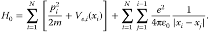
In this equation, Ve,i
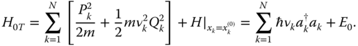
is the trapping potential that confines the kth ion, and it may be the same for all of them if stored in a common linear trap (1) or may change from ion to ion as in the case of microtraps (16). If we expand the previous Hamiltonian around the equilibrium configuration, given by (∂H/∂xi
) ![]() , and find out the normal modes for the resulting system of coupled oscillators, we obtain
, and find out the normal modes for the resulting system of coupled oscillators, we obtain
The new collective coordinates, Qk
= Mik
[xi − ![]() ] and Pk
= Mikpi
, are defined in terms of an orthogonal transformation, Mt
= M
−1, and they are usually replaced by the corresponding Fock operators Qk
=
] and Pk
= Mikpi
, are defined in terms of an orthogonal transformation, Mt
= M
−1, and they are usually replaced by the corresponding Fock operators Qk
= ![]() and Pk
=
and Pk
= ![]() . For instance, for two ions in a linear Paul trap we have two modes, a center of mass mode with frequency equal to the trap frequency, νcm
= ν, and a stretch mode with incommensurate frequency νr
=
. For instance, for two ions in a linear Paul trap we have two modes, a center of mass mode with frequency equal to the trap frequency, νcm
= ν, and a stretch mode with incommensurate frequency νr
= ![]() ν. Finally, E
0 denotes the energy of the ions in the equilibrium configuration.
ν. Finally, E
0 denotes the energy of the ions in the equilibrium configuration.
23.2.2 Internal Degrees of Freedom and Atom–Laser Interaction
We will model the internal electronic structure of the ion using a two‐level system, |g〉 and |e〉. These two long‐lived levels are connected by a dipole‐forbidden transition, and since they are used to store the quantum information, they are also denoted as |0〉 and |1〉. We will study what happens when a laser driving the transition |g〉 → |e〉 is on. If the interaction time between the atom and the laser beam is much longer than the lifetime of the state |e〉, we can neglect spontaneous emission. Then, in a frame rotating with the laser frequency, the Hamiltonian modeling the process will be (ℏ = 1)
for standing‐wave and traveling‐wave configurations, respectively. Here, δ = ωL − ωrg is the laser detuning from the internal transition; Ω is the Rabi frequency; and k is the wavevector of the photons. The sign ± denotes that the laser plane wave propagates in the positive or negative x direction. Finally, φ depends on the position of the trap in the laser standing wave.
23.2.3 Lamb–Dicke Limit and Sideband Transitions
In some parts of this chapter, we will confine our discussion to the Lamb–Dicke limit, that is, to the limit where the ion motion is restricted to a region much smaller than the wavelength of the light exciting a given transition (19): k|xk − ![]() | ≪ 1. This allows us to expand the Hamiltonian (23.3) up to the first order in terms of the Lamb–Dicke parameters ηj
= kαj
, where αj
= 1/(2mνj
)1/2 is the size of the ground state of jth vibrational mode. For a single trapped ion, we have the first order in η
| ≪ 1. This allows us to expand the Hamiltonian (23.3) up to the first order in terms of the Lamb–Dicke parameters ηj
= kαj
, where αj
= 1/(2mνj
)1/2 is the size of the ground state of jth vibrational mode. For a single trapped ion, we have the first order in η
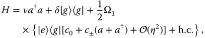
where c 0 = 1, c± = ±iη and c 0 = sin(φ), c± = η cos(φ) are for a traveling‐ and standing‐wave configuration, respectively.
This model can be further simplified if the laser field is sufficiently weak so that only pairs of bare atom + trap levels are coupled resonantly (Figure 23.1). Let us introduce the spin‐1/2 notation σz
= |e〉〈r| − |g〉〈g|, σ
+ = |e〉〈g|. We denote by |g, n〉 and |e, n〉 the eigenstates of the bare Hamiltonian H
bare = νa
†
a − ![]() δσz
, where the internal two‐level system is in the ground or excited state and n is the occupation number of the harmonic oscillator. Whenever the laser is tuned to one of the “motional sidebands,” that is for δ = 0, ν, 2ν, …, the pairs of |g, n〉 and |e, n + k〉 (k = 0, 1, 2, …) become degenerate. For example, right on atomic resonance, δ ≃ 0, transitions changing the harmonic oscillator quantum number n are off‐resonance and can be neglected. In this case, the Hamiltonian (23.3) can be approximated by
δσz
, where the internal two‐level system is in the ground or excited state and n is the occupation number of the harmonic oscillator. Whenever the laser is tuned to one of the “motional sidebands,” that is for δ = 0, ν, 2ν, …, the pairs of |g, n〉 and |e, n + k〉 (k = 0, 1, 2, …) become degenerate. For example, right on atomic resonance, δ ≃ 0, transitions changing the harmonic oscillator quantum number n are off‐resonance and can be neglected. In this case, the Hamiltonian (23.3) can be approximated by
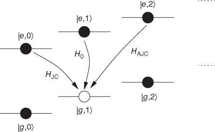
Figure 23.1 Coupling of the atom + trap levels according to the Hamiltonians Eqs. 23.5,23.6,23.7, respectively, in the lowest order Lamb–Dicke expansion.
On the other hand, for laser frequencies close to the lower motional sideband resonance δ ≃ −ν, only transitions decreasing the quantum number n by one are important, and (23.3) can be approximated by a Hamiltonian of the Jaynes–Cummings type:
Similarly, for δ ∼ +ν, only transitions increasing the quantum number n by one contribute, so that (23.3) can be approximated by the anti‐Jaynes–Cummings Hamiltonian
For all these approximations to be valid we require that the effective Rabi frequencies to the nonresonant states be much smaller than the trap frequency (c 0,± Ω/ν)2 ≪ 1, that is, we must spectroscopically resolve the motional sidebands. Note, in particular, that for an ion at the node of a standing light wave, corrections to H JC are of the order (ηΩ/ν)2 ≪ 1, that is, the conditions of validity are greatly relaxed.
23.2.4 Single‐Qubit Operations and State Measurement
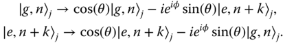
The eigenstates of the Hamiltonians H 0, H JC, and H AJC are the dressed states familiar from cavity QED, which are obtained by diagonalizing the 2 × 2 matrices of nearly degenerate states, |g, n〉 and |e, n + k〉 with k = 0, −1, +1, respectively. Using each of these possible configurations, one can perform arbitrary rotations on these subspaces
In particular, when δ = k = 0 this can be used to make any single qubit unitary transformation. However, one may also swap information from the internal degrees of freedom to the motional ones, as in (α|g〉 + β|e〉)|0〉 → |g〉(α|0〉 + β|1〉) (Figure 23.2a) or introduce conditional phases. These types of operations are the basic ingredients for many quantum gates and in particular for the gate (1) explained below.
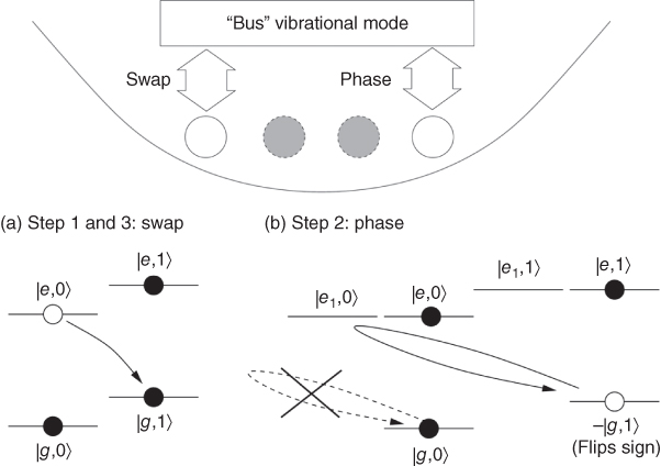
Figure 23.2 Ion‐trap quantum computer '95. (a) First step according to Eq. 23.9: the qubit of the first atom is swapped to the photonic data bus with a π‐pulse on the lower motional sideband, (b) second step: the state |g, 1〉 acquires a minus sign due to a 2π‐rotation via the auxiliary atomic level |e 1〉 on the lower motional sideband. By combining both operations, the quantum information can be transmitted from the internal state of the ions to a vibrational mode (the “bus”). This allows selected pairs of ions to see each other and to produce a two‐qubit gate.
Implementation of quantum information protocols also requires measurement of the internal state of the atom. For ions, this can be done with essentially 100% efficiency using the method of quantum jumps (12,20). The theoretical understanding of quantum jumps is based on the continuous measurement theory, and we refer to (12) for a detailed mathematical description of the underlying theory. For our purpose, it suffices to summarize the results as follows. Consider a single ion prepared initially in a superposition state on the metastable transition, α|g〉 + β|e〉. Switching on a laser tuned to a strongly dissipative transition |g〉 → |e 1〉 involving some short‐lived atomic state |e 1〉, will give with probability |α| 2 a burst of photon emissions |e 1〉 → |g〉 on the time scale 1/Γ (Γ is the spontaneous emission rate), or with probability |β| 2 the appearance on an emission window on the strong line. Measuring an emission window, or no window, thus corresponds to a projective measurement of |e〉 or |g〉.
23.2.5 The Cirac–Zoller Gate '95
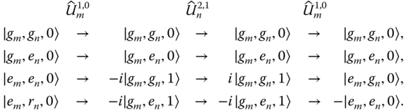
The original two‐qubit gate from Ref. (1) can be understood as the composition of two fundamental operations between the internal state of the ions and a single vibrational mode or “bus” mode. For this purpose, the mediating vibrational mode (typically the center of mass) has to be cooled to the ground state (21,22). The first operation is labeled ![]() and it transfers a qubit from the mth ion to the bus. As described in Eq. 23.8, the activation of the bus mode is done with a π‐pulse performs the swap |e, n − 1〉 ↔ |g, n〉, leaving the state |g, 0〉 untouched (Figure 23.2a). The second operation, denoted Un
2,0, uses the second ion that participates in the gate. This time the operation is done via a third auxiliary atomic state |e
1〉, performing a 2π rotation on the two‐level system |g, 1〉 ↔ |e
1
, 0〉 (Figure 23.2b). The result is a phase gate that changes the sign of the quantum state only when the nth ion is in the internal state g and the bus mode has one phonon. The composition of both unitaries produces a phase gate between the internal state of the ions, while leaving the bus state untouched
and it transfers a qubit from the mth ion to the bus. As described in Eq. 23.8, the activation of the bus mode is done with a π‐pulse performs the swap |e, n − 1〉 ↔ |g, n〉, leaving the state |g, 0〉 untouched (Figure 23.2a). The second operation, denoted Un
2,0, uses the second ion that participates in the gate. This time the operation is done via a third auxiliary atomic state |e
1〉, performing a 2π rotation on the two‐level system |g, 1〉 ↔ |e
1
, 0〉 (Figure 23.2b). The result is a phase gate that changes the sign of the quantum state only when the nth ion is in the internal state g and the bus mode has one phonon. The composition of both unitaries produces a phase gate between the internal state of the ions, while leaving the bus state untouched
This phase gate is more concisely written as |ɛ
1〉|ɛ
2〉 → ![]() and it is equivalent to a controlled‐NOT up to single‐qubit rotations. Together with the single‐qubit operations and measurements, these are all the ingredients required to implement small quantum computations (15).
and it is equivalent to a controlled‐NOT up to single‐qubit rotations. Together with the single‐qubit operations and measurements, these are all the ingredients required to implement small quantum computations (15).
The previous setup has several limitations. First, the bus mode has to be cooled to the zero phonon limit, a process that takes time and makes the gate sensitive to heating. Second, it requires being able to address individual ions during realization of the two‐qubit gate. This limits the tightness of the traps that can be used and thus the speed. Finally, the fact that we cannot excite more than one phonon, the need to resolve a sideband (i.e., to excite only one mode and leave the other untouched), and the Mössbauer effect, 1 impose severe limits in the intensity of the coupling between internal and motional degrees of freedom and make the gate slow.
23.2.6 The Cirac–Zoller Gate
While in the ion‐trap '95 scheme a two‐qubit gate was realized using the collective phonon mode as an auxiliary quantum degree of freedom, we now describe briefly a version on an ion‐trap computer in which entanglement is achieved by designing an internal‐state dependent two‐body interaction between the ions (16,23). This proposal has the advantage of being conceptually simpler (e.g., there is no zero temperature requirement), and obviously scalable. The model assumes that the N ions are stored in an array of microtraps: independent harmonic potential wells, separated by some distance d that is large enough so that the ions can be individually addressed (Figure 23.3a). Similar to the ion‐trap '95 proposal, information is stored using long‐lived internal atomic states and single‐qubit operations are performed by addressing individually the ions with a laser.
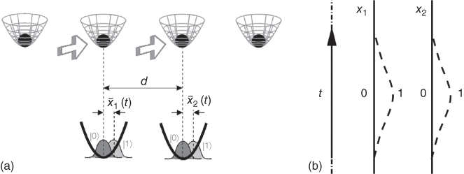
Figure 23.3 (a) Ions stored in an array of microtraps. By addressing two adjacent ions with an external field the ion wavepacket is displaced conditional to its internal state. (b) Trajectories of the qubits as a function of time. Depending on the internal state different phases are accumulated.
The two‐qubit gate is then performed between neighboring ions adiabatically. One must apply a standing wave of off‐resonance laser light on both ions. The dipole force exerted by the light can be designed so that it only pushes ions that are on one of the qubit states, say |1〉. Switching on and off the state‐dependent force is equivalent to displacing the center of the microtraps (Figure 23.3a), so that, depending on the internal state, the ions will approach each other or become more separated (Figure 23.3b). If the whole process is done adiabatically, the motional state of the ions will be restored. However, according to the adiabatic theorem, the quantum state will have acquired a different phase, which depends on the Coulomb interaction experienced by the ions during the pushing. This way, by tuning the duration of the gate, we can produce a phase gate |ɛ
1〉|ɛ
2〉 → ![]() |ɛ
1〉|ɛ
2〉.
|ɛ
1〉|ɛ
2〉.
In order to analyze this in a more quantitative way, we consider two ions 1 and 2 of mass m confined by two harmonic traps of frequency ν in one dimension (Figure 23.3a). A standing wave of off‐resonance light induces an AC‐Stark shift and thus a dipole force on one of the internal states, |1〉. The expression of this potential is similar to Eq. 23.3a. By placing the ions in the node of the standing wave, the force becomes approximately linear and the effective Hamiltonian can be written as HF
= ∑
i=1,2 − Fi
(t)xi |1〉〈1| + ![]() . The total potential experienced by the ions is
. The total potential experienced by the ions is
where ![]() (t) ∼ Fi
/mν
2 is the state‐dependent displacement induced by the force. We will impose that the ions do not come too close to each other, |x
1,2
| ≪ d, so that the Coulomb energy remains small compared to the trapping potentials, ɛ|x
1 x
2
|/
(t) ∼ Fi
/mν
2 is the state‐dependent displacement induced by the force. We will impose that the ions do not come too close to each other, |x
1,2
| ≪ d, so that the Coulomb energy remains small compared to the trapping potentials, ɛ|x
1 x
2
|/![]() ≪ 1. Furthermore, we will assume that the motional state of the pushed ions changes adiabatically with the potential. Expanding the Coulomb term in powers of
≪ 1. Furthermore, we will assume that the motional state of the pushed ions changes adiabatically with the potential. Expanding the Coulomb term in powers of ![]() produces a term −mω
2
ɛx
1
x
2 in the potential 23.10. It is this term that is responsible for entangling atoms, giving rise to a conditional phase shift, which can be simply interpreted as arising from the energy shifts due to the Coulomb interactions of atoms accumulated on different trajectories according to their internal states (Figure 23.3b),
produces a term −mω
2
ɛx
1
x
2 in the potential 23.10. It is this term that is responsible for entangling atoms, giving rise to a conditional phase shift, which can be simply interpreted as arising from the energy shifts due to the Coulomb interactions of atoms accumulated on different trajectories according to their internal states (Figure 23.3b),
where the four terms are due to atoms in |1〉1 |1〉2, |1〉1 |0〉2, |0〉1 |1〉2, and |0〉1 |0〉2, respectively.
The phase acquired by the ions depends only on mean displacement of the atomic wavepacket and thus it is insensitive to the temperature (the width of the wavepacket), which will appear only in the problem in higher orders in x 1,2/d of our expansion of the potential 23.10, or in the cases of nonadiabaticity. This feature means that this gate can be used in the type of setups considered for scalable quantum computing, because it is not required to cool the ions completely after bringing them to the interaction region. However, the fact that the gate operates in the adiabatic regime, means that it will be much slower than the period of the trap. A detailed theory of this proposal including an analysis of imperfections can be found in (23).
23.2.7 Optimal Gates Based on Quantum Control
With the number of different proposals for performing two‐qubit quantum gates with ions (1 5–8,11,16,24), the question of what are the ultimate limits of quantum computing in these systems remained open. For instance, a quick inspection of the literature reveals that most gates require a time much larger than the period of the trap, Ref. (5) being an exception. This question was answered in Ref. (9), where the main stopper of current proposals was identified to be the need of addressing a single vibrational mode. Following the ideas of Poyatos et al. (5), this work suggests using all vibrational modes, combined with state‐dependent forces to engineer a phase gate between the ions.
The background idea is very simple, and begins with a single forced ion in a harmonic trap. The model being considered is
and F(t)σz represents the state‐dependent force acting on the ion. This problem can be integrated exactly, and the result is that the force F(t) distorts the circular orbits on phase space, (x, p), adding some area to them (Figure 23.4a). If the force is properly designed, the motional state of the ion will be restored (Figure 23.4b) and the final quantum state will be
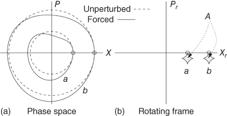
Figure 23.4 (a) Orbits in phase space of a single ion in a harmonic trap, either unforced (dashed) or subject to a time‐dependent force (solid). (b) Similar picture but on a rotating frame of reference.
This unitary evolution is made of two terms: one which would even be present in the free, unforced case, plus an additional dynamical phase, eiA , that depends on the area covered in the rotating frame of reference (Figure 23.4b).
First, if we had not one ion but two, both of them coupled to a common vibrational mode, the phase would depend on the product ![]() , and by tuning the area A one could produce a phase gate, |ɛ
1
, ɛ
2〉 →
, and by tuning the area A one could produce a phase gate, |ɛ
1
, ɛ
2〉 → ![]() |ɛ
1
, ɛ
2〉. This idea was already used experimentally in (14) to generate a two‐qubit gate in an ion trap. Second and most important, the area and the phase obtained by the ions do not depend on the motional state, which is also “restored” at the end of the process, making the gate extremely robust. However, in real experiments we do not have a single vibrational mode, and implementing the previous proposal requires once more addressing a single sideband (14), which makes the gate as slow as the pushing gate.
|ɛ
1
, ɛ
2〉. This idea was already used experimentally in (14) to generate a two‐qubit gate in an ion trap. Second and most important, the area and the phase obtained by the ions do not depend on the motional state, which is also “restored” at the end of the process, making the gate extremely robust. However, in real experiments we do not have a single vibrational mode, and implementing the previous proposal requires once more addressing a single sideband (14), which makes the gate as slow as the pushing gate.
To solve the problem of speed, we put in the second ingredient, which is coherent quantum control. The goal is to achieve a certain unitary transformation using all degrees of freedom in the trapped ion system. For that, we are free to design the time dependence of all controlling parameters in our experiment: which in our case are the state‐dependent forces applied on the ions. Notably, the model in our hands is completely integrable (10) and the control problem is rather easy. In the case of two ions we can use a common force,2 and if this force satisfies two commensurability conditions
the evolution of the ions can be decomposed into a phase operation and a global rotation
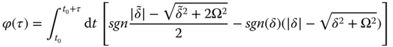
Here, acm and ar stand for the center of mass and stretch modes, and φ is the total phase
In Ref. (9), it was suggested to use ultrashort laser pulses to kick the ions instantaneously, so that the forces may actually be written as a sequence of delta kicks
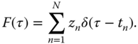
Each protocol is uniquely characterized by the intensity of the kicks, zj , and the instant in which they are applied, tj . This parameterization was used in Ref. (9) to design a protocol that produces a phase gate within a period of the trap, T ∼ 1/ν, using only four kicks (Figure 23.5). Furthermore, a similar protocol was found that, within this simplified model, produces the phase gate as fast as wished. However, in practice, making faster gates involves also stronger forces and larger displacements of the ions. These larger displacements are then a source of error, either because the ions approach each other so much that the harmonic model 23.2 breaks down, or because there is some dissipation on the vibrational degrees of freedom that causes an exponential decay of the fidelity. For a deeper analysis of the errors, a generalization to many‐ions setups and continuous forces, we refer the reader to (10).
Figure 23.5
(a) Trajectory in phase space of the center‐of‐mass state of the ion (Xc
, Pc
) (where  = 〈a〉) during the two‐qubit gate (solid line), connecting the initial state (black filled circle) to the final state (gray filled circle) at the gate time T. The time evolution consists of a sequence of kicks (vertical displacements), which are interspersed with free harmonic oscillator evolution (motion along the arcs). A pulse sequence satisfying the commensurability condition (Eq. 23.14 guarantees that the final phase space point is restored to the one corresponding to a free harmonic evolution (dashed circle). The particular pulse sequence plotted corresponds to a four pulse sequence given in the text (Protocol I). (b) It shows how the laser pulses (bars) distribute in time for this scheme.
23.3 Trapped Neutral Atoms
The creation of atomic Bose–Einstein condensates (BEC) and degenerate Fermi gases marks a milestone in the history of atomic physics. These degenerate gases enable a range of novel possibilities for applications exploiting ultracold trapped neutral atoms. One of the most promising experiments for future applications is the loading of a BEC into an optical lattice (25–27). Optical lattices are periodic conservative trapping potentials that are created by interference of traveling laser beams yielding standing laser waves in each direction (see Figure 23.6). The laser light induces AC–Stark shift in atoms and thus acts as a conservative periodic potential (28). The usage of a BEC for loading has the advantage that atoms are ultracold at temperatures very close to zero so that they practically behave as if their temperature was T = 0; in particular all of them occupy the lowest Bloch band. Furthermore, the large density of atoms loaded from a BEC enables a filling of few particles per site n ≳ 1 while laser‐cooled atoms loaded into an optical lattice typically only allow a filling factor smaller than one. The resulting competition of atom hopping between neighboring sites and repulsion of two atoms occupying the same lattice site can be used to induce a quantum phase transition from a superfluid (SF) atom state to a Mott insulator (MI) state where each site is filled by exactly one atom thus realizing a regular array of qubits. Further manipulation of atoms using external fields (e.g., laser) then allows quantum information processing on the qubits.
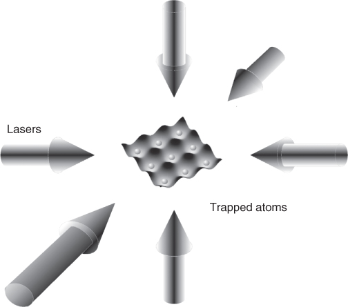
Figure 23.6 Laser setup and resulting optical lattice configuration in 3D.
23.3.1 Optical Lattices
In this section, we present several examples of different laser–atom configurations for the realization of a variety of trapping potentials, in particular, periodic optical lattices with different geometries, and even trapping potentials whose shape depends on the internal (hyperfine) state of the atom. These setups are the basis for realizing quantum memories and quantum gates. In our derivations, we will neglect spontaneous emission and later establish the consistency of this approximation by giving an estimate for the rate at which photons are spontaneously emitted in a typical optical lattice setup.
23.3.1.1 Optical Potentials
The Hamiltonian of an atom of mass m is given by HA
= p
2
/2m + ![]() . Here p is the center of mass momentum operator and |ej
〉 denotes the internal atomic states with energies ωj
(setting ℏ ≡ 1). We assume the atom to initially occupy a metastable internal state |e
0〉 ≡ |a〉 that defines the point of zero energy. The atom is subject to a classical laser field with electric field E(x
,t) = E(x
, t)ɛ exp(−iωt), where ω is the frequency and ɛ the polarization vector of the laser. The amplitude of the electric field E(x
, t) is varying slowly in time t compared to 1/ω and slowly in space x compared to the size of the atom. In this situation, the interaction between atom and laser is adequately described in dipole approximation by the Hamiltonian H
dip = −μ
E(x
, t) + h
.c
., where μ is the dipole operator of the atom. We assume the laser to be far detuned from any optical transition so that no significant population is transferred from |a〉 to any of the other internal atomic states via H
dip. We can thus treat the additional atomic levels in perturbation theory and eliminate them from the dynamics. In doing so, we find the AC‐Stark shift of the internal state |a〉 in the form of a conservative potential V(x) whose strength is determined by the atomic dipole operator and the properties of the laser light at the center of mass position x of the atom. In particular, V(x) is proportional to the laser intensity |E(x
, t)|
2. Under these conditions, the motion of the atom is governed by the Hamiltonian H = p
2/2m + V(x).
. Here p is the center of mass momentum operator and |ej
〉 denotes the internal atomic states with energies ωj
(setting ℏ ≡ 1). We assume the atom to initially occupy a metastable internal state |e
0〉 ≡ |a〉 that defines the point of zero energy. The atom is subject to a classical laser field with electric field E(x
,t) = E(x
, t)ɛ exp(−iωt), where ω is the frequency and ɛ the polarization vector of the laser. The amplitude of the electric field E(x
, t) is varying slowly in time t compared to 1/ω and slowly in space x compared to the size of the atom. In this situation, the interaction between atom and laser is adequately described in dipole approximation by the Hamiltonian H
dip = −μ
E(x
, t) + h
.c
., where μ is the dipole operator of the atom. We assume the laser to be far detuned from any optical transition so that no significant population is transferred from |a〉 to any of the other internal atomic states via H
dip. We can thus treat the additional atomic levels in perturbation theory and eliminate them from the dynamics. In doing so, we find the AC‐Stark shift of the internal state |a〉 in the form of a conservative potential V(x) whose strength is determined by the atomic dipole operator and the properties of the laser light at the center of mass position x of the atom. In particular, V(x) is proportional to the laser intensity |E(x
, t)|
2. Under these conditions, the motion of the atom is governed by the Hamiltonian H = p
2/2m + V(x).
Let us now specialize the situation to the case where the dominant contribution to the optical potential arises from one excited atomic level |e〉 only. In a frame rotating with the laser frequency the Hamiltonian of the atom is approximately given by HA = p 2/2m + δ |e〉 〈e|, where δ = ωe − ω is the detuning of the laser from the atomic transition |e〉 ↔ |a〉. The dominant contribution to the atom–laser interaction neglecting all quickly oscillating terms (i.e., in the rotating wave approximation) is given by H dip = Ω(x) |e〉 〈a|/2 + h .c. Here Ω = −2E(x , t)〈e|μɛ|a〉 is the so‐called Rabi frequency driving the transitions between the two atomic levels. For large detuning δ ≫ Ω adiabatically eliminating the level |e〉 yields the explicit expression V(x) = |Ω(x)| 2/4δ for the optical potential. The population transferred to the excited level |e〉 by the laser is given by |Ω(x)| 2/4δ 2, and this is the reason why we require Ω(x) ≪ δ for our adiabatic elimination to be valid.
23.3.1.2 Periodic Lattices
For creating an optical lattice potential, we start by superimposing two counter‐propagating running‐wave laser beams with E± (x, t) = E 0 exp(±ikx) propagating in the x‐direction with amplitude E 0, wave number k and wavelength λ = 2π/k. They create an optical potential V(x) ∝ cos2(kx) in one dimension with periodicity a = λ/2. Using two further pairs of laser beams propagating in y‐ and z‐directions, respectively, a full three‐dimensional periodic trapping potential of the form
is realized. The depth of this lattice in each direction is determined by the intensity of the corresponding pair of laser beams that is easily controlled in an experiment.
23.3.1.3 Bloch Bands and Wannier Functions
For simplicity, we only consider one spatial dimension in Eq. 23.18 and write down the Bloch functions ![]() with q the quasi momentum and n the band index. The corresponding eigenenergies
with q the quasi momentum and n the band index. The corresponding eigenenergies ![]() for different depths of the lattice V
0
/ER
in units of the recoil energy ER
= k
2
/2m are shown in Figure 23.7. Already for a moderate lattice depth of a few recoil the energy separation between the lowest lying bands is much larger than their width. In this case, a good approximation for the gap between these bands is given by the oscillation frequency ωT
of a particle trapped close to one of the minima xj
(≡lattice site) of the optical potential. Approximating the lattice around a minimum by a harmonic oscillator we find ωT
=
for different depths of the lattice V
0
/ER
in units of the recoil energy ER
= k
2
/2m are shown in Figure 23.7. Already for a moderate lattice depth of a few recoil the energy separation between the lowest lying bands is much larger than their width. In this case, a good approximation for the gap between these bands is given by the oscillation frequency ωT
of a particle trapped close to one of the minima xj
(≡lattice site) of the optical potential. Approximating the lattice around a minimum by a harmonic oscillator we find ωT
= ![]() (29).
(29).
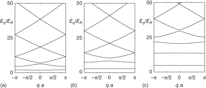
Figure 23.7 Band structure of an optical lattice of the form V 0(x) = V 0 cos2(kx) for different depths of the potential. (a) V 0 = 5ER , (b) V 0 = 10ER , and (c) V 0 = 25ER .
The dynamics of particles moving in the lowest‐lying, well‐separated bands will be described using the Wannier functions. These are complete sets of orthogonal normalized real‐mode functions for each band n. For properly chosen phases of the ![]() (x) the Wannier functions optimally localized at lattice site xj
are defined by (30)
(x) the Wannier functions optimally localized at lattice site xj
are defined by (30)
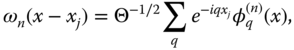
where Θ is a normalization constant. Note that for V
0 → ∞ and fixed k the Wannier function wn
(x) tends toward the wavefunction of the nth excited state of a harmonic oscillator with the ground state size a
0 = ![]() . We will use the Wannier functions to describe particles trapped in the lattice since they allow (i) to attribute a mean position xj
to the particles in a given mode and (ii) to easily account for local interactions between particles because the dominant contribution to the interaction energy arises from particles occupying the same lattice site xj
.
. We will use the Wannier functions to describe particles trapped in the lattice since they allow (i) to attribute a mean position xj
to the particles in a given mode and (ii) to easily account for local interactions between particles because the dominant contribution to the interaction energy arises from particles occupying the same lattice site xj
.
23.3.1.4 Lattice Geometry and Site Offset
The lattice site positions x
j
determine the lattice geometry. For instance, the above arrangement of three pairs of orthogonal laser beams leads to a simple cubic lattice (shown in Figure 23.8a). Since the laser setup is very versatile different lattice geometries can be achieved easily. As an example, consider three laser beams propagating at angles 2π/3 with respect to each other in the xy‐plane and all of them being polarized in the z direction. The resulting lattice potential is given by V(x) ∝ 3 + 4 cos(3kx/2) cos(![]() ky/2) + 2 cos(
ky/2) + 2 cos(![]() ky), which is a triangular lattice in two dimensions. An additional pair of lasers in the z direction can be used to create localized lattice sites (cf. Figure 23.8b). Furthermore, as will be discussed later in Section 23.3.2, the motion of atoms can be restricted to two or even one spatial dimension by large laser intensities. As will be shown, it is thus possible to create truly one‐ and two‐dimensional lattice models as indicated in Figure 23.8b and c respectively. The offset of the lattice sites can be manipulated through a superimposed magnetic trapping field or Stark shifts introduced by additional lasers. In particular, regular patterns are useful for quantum computing as they exploit the inherent scalability of optical lattice setups.
ky), which is a triangular lattice in two dimensions. An additional pair of lasers in the z direction can be used to create localized lattice sites (cf. Figure 23.8b). Furthermore, as will be discussed later in Section 23.3.2, the motion of atoms can be restricted to two or even one spatial dimension by large laser intensities. As will be shown, it is thus possible to create truly one‐ and two‐dimensional lattice models as indicated in Figure 23.8b and c respectively. The offset of the lattice sites can be manipulated through a superimposed magnetic trapping field or Stark shifts introduced by additional lasers. In particular, regular patterns are useful for quantum computing as they exploit the inherent scalability of optical lattice setups.
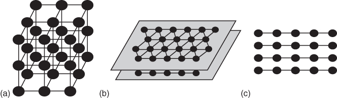
Figure 23.8 (a) Simple three‐dimensional cubic lattice. (b) Sheets of a two‐dimensional triangular lattices. (c) Set of one‐dimensional lattice tubes. In (a)–(c) tunneling of atoms through the optical potential barriers is only possible between sites that are connected by lines.
23.3.1.5 State‐Dependent Lattices
As already mentioned above, the strength of the optical potential crucially depends on the atomic dipole moment between the internal states involved. Thus, we can exploit selection rules for optical transitions to create differing traps for different internal states of the atom (31–33). We will illustrate this by an example that is particularly relevant in what follows. We consider an atom with the fine structure shown in Figure 23.9a, like for example, 23Na or 87Rb, interacting with two circularly polarized laser beams. The right circularly polarized laser σ
+ couples the level S
1/2 with ms
= −1/2 to two excited levels P
1/2 and P
3/2 with ms
= 1/2 and detunings of opposite sign. The respective optical potentials add up. The strength of the resulting AC‐Stark shift is shown in Figure 23.9b as a function of the laser frequency ω. For ω = ωL, the two contributions cancel. The same can be achieved for the σ−
laser acting on the S
1/2 level with ms
= 1/2. Therefore, at ω = ωL
the AC‐Stark shift of the levels S
1/2 with ms
= ±1/2 are purely due to σ±
polarized light that we denote by V±
(x). The corresponding level shifts of the hyperfine states in the S
1/2 manifold (shown in Figure 23.9a) are related to V±
(x) by the Clebsch–Gordan coefficients, for example, ![]() (x) = V
+(x),
(x) = V
+(x), ![]() (x) = 3V
+(x)/4 + V−
(x)/4, and
(x) = 3V
+(x)/4 + V−
(x)/4, and ![]() (x) = V
+(x)/4 + 3V−
(x)/4.
(x) = V
+(x)/4 + 3V−
(x)/4.
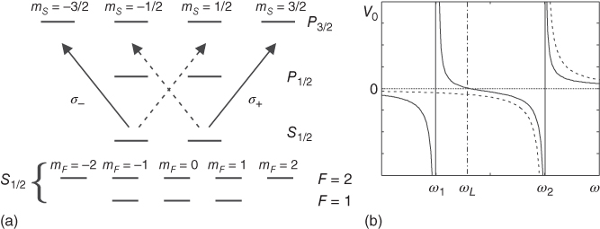
Figure 23.9 (a) Atomic fine and hyperfine structure of the most commonly used alkali atoms 23Na and 87Rb. (b) Schematic AC‐Stark shift of the atomic level S 1/2 with ms = 1/2 (dashed curve) and with ms = −1/2 (solid curve) due to the laser beam σ + as a function of the laser frequency ω. The AC‐Stark shift of the level S 1/2 with ms = −1/2 can be made 0 by choosing the laser frequency ω = ωL .
23.3.1.6 State Selectively Moving the Lattice
The two standing waves σ± can be produced out of two running counter‐propagating waves with the same intensity as shown in Figure 23.10. Moreover, it is possible to move nodes of the resulting standing waves by changing the angle of the polarization between the two running waves (31). Let {e 1, e 2, e 3} be three unit vectors in space pointing along the {x, y, z} direction, respectively. The position‐dependent part of the electric field of the two running waves E 1,2 is given by E 1 ∝ eikx (cos(ϕ)e 3 + sin(ϕ)e 2), E 2 ∝ e−ikx (cos(ϕ)e 3 − sin(ϕ)e 2). The sum of the two electric fields is thus E 1 + E 2 ∝ cos(kx − ϕ)σ− − cos(kx + ϕ)σ +, where σ± = e 2 ± ie 3 and the resulting optical potentials are given by
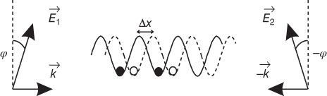
Figure 23.10 Laser configuration for a state selective optical potential. Two standing circular polarized standing waves are produced out of two counter‐propagating running waves with an angle 2ϕ between their polarization axes. The lattice sites for different internal states (indicated by closed and open circles) are shifted by Δx = 2ϕ/k.
By changing the angle ϕ, it is therefore possible to move the nodes of the two standing waves in the opposite directions. Since these two standing waves act as internal state‐dependent potentials for the hyperfine states the optical lattice can be moved in the opposite directions for different internal hyperfine states.
23.3.1.7 Validity
In all of the above calculations, we have only considered the coherent interactions of an atom with laser light. Any incoherent scattering processes that lead to spontaneous emission were neglected. We will now establish the validity of this approximation by estimating the mean rate Γeff of spontaneous photon emission from an atom trapped in the lowest vibrational state of the optical lattice. This rate of spontaneous emission is given by the product of the life time Γ of the excited state and the probability of the atom occupying this state. In the case of a blue detuned optical lattice (dark optical lattice) δ < 0, the potential minima coincide with the points of no light intensity and we find the effective spontaneous emission rate Γeff ≈ −ΓωT /4δ. If the lattice is red detuned (bright optical lattice) δ > 0, the potential minima match the points of maximum light intensity and we find Γeff ≈ ΓV 0/δ. Since V 0 > ωT the spontaneous emission in a red detuned optical lattice will always be more significant than in a blue lattice, however, as long as V 0 ≪ δ spontaneous emission does not play a significant role.
23.3.1.8 Typical Numerical Values
In a typical blue detuned optical lattice, with λ = 514 nm for 23Na atoms (S 1/2 − P 3/2 transition at λ 2 = 589 nm and Γ = 2π × 10 MHz), the recoil energy is ER ≈ 2π × 33 kHz and the detuning from the atomic resonance is δ ≈ −2 .3 × 109 ER . A lattice with depth V 0 = 25ER leads to a trapping frequency of ωT = 10ER yielding a spontaneous emission rate of Γeff ≈ 10 −2 /s while experiments are typically carried out in times shorter than one second. Therefore, spontaneous emission does not play a significant role in such experiments.
23.3.2 The (Bose) Hubbard Hamiltonian
We consider a gas of interacting particles moving in an optical lattice. Starting from the full many body Hamiltonian including local two particle interactions, we first give brief derivation of the BHM (29,34) and present related models that can be realized in an optical lattice. Then, we proceed by discussing adiabatic and irreversible schemes for loading the lattice with ultracold atoms. Throughout, we will concentrate on bosonic atoms. Similar derivations for fermions lead to quantum registers realized by fermions (33,35).
23.3.2.1 The (Bose) Hubbard Model
The Hamiltonian of a weakly interacting gas in an optical lattice is
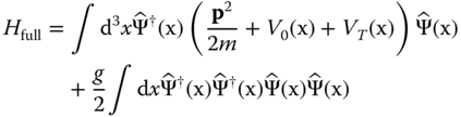
with ![]() the bosonic field operator for atoms in a given internal atomic state |b〉 and VT
(x) a (slowly varying compared to the optical lattice V
0 (x)) external trapping potential, for example, a magnetic trap or a superlattice potential. The parameter g is the interaction strength between two atomic particles. Only if atoms interact via s‐wave scattering, it is given by g = 4πas/m with as
the s‐wave scattering length. We assume all particles to be in the lowest band of the optical lattice and expand the field operator in terms of the Wannier functions
the bosonic field operator for atoms in a given internal atomic state |b〉 and VT
(x) a (slowly varying compared to the optical lattice V
0 (x)) external trapping potential, for example, a magnetic trap or a superlattice potential. The parameter g is the interaction strength between two atomic particles. Only if atoms interact via s‐wave scattering, it is given by g = 4πas/m with as
the s‐wave scattering length. We assume all particles to be in the lowest band of the optical lattice and expand the field operator in terms of the Wannier functions ![]() , where
, where ![]() is the destruction operator for a particle in site x
i
. We find
is the destruction operator for a particle in site x
i
. We find
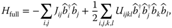
where
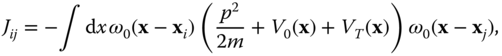
and
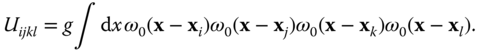
The numerical values for the offsite interaction matrix elements Uijkl involving Wannier functions centered at different lattice sites as well as tunneling matrix elements Jij to sites other than nearest neighbors (note that diagonal tunneling is not allowed in a cubic lattice since the Wannier functions are orthogonal) are small compared to onsite interactions U 0000 ≡ U and nearest neighbor tunneling J 01 ≡ J for reasonably deep lattices V 0 ≳ 5ER . We can therefore neglect them and for an isotropic cubic optical lattice arrive at the standard Bose–Hubbard Hamiltonian
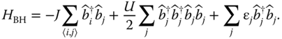
Here 〈i, j〉 denotes the sum over nearest neighbors and the terms ɛj = V T(x j ) arise from the additional trapping potential. The physics described by H BH is schematically shown in Figure 23.11a. Particles gain an energy of J by hopping from one site to the next while two particles occupying the same lattice site provide an interaction energy U. An increase in the lattice depth V 0 leads to higher barriers between the lattice sites decreasing the hopping energy J as shown in Figure 23.11b. At the same time, two particles occupying the same lattice site become more compressed, which increases their repulsive energy U (cf. Figure 23.11b).
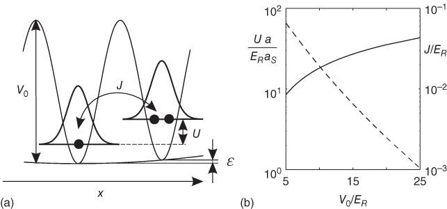
Figure 23.11 (a) Interpretation of the BHM in an optical lattice as discussed in the text. (b) Plot of scaled onsite interaction U/ER multiplied by a/as (≫1) (solid line with axis on left‐hand side of graph) and J/ER (dashed line, with axis on right‐hand side of graph) as a function of V 0 /ER ≡ V x,y,z0/ER (for a cubic 3D lattice).
23.3.2.2 Tunneling Term J
In the case of an ideal gas, where U = 0, the eigenstates of H
BH are easily found for ɛi
= 0 and periodic boundary conditions. From the eigenvalue equation ![]() = −2J cos(qa), we find that 4J is the height of the lowest Bloch band. Furthermore, we see that the energy is minimized for q = 0 and therefore particles in the ground state are delocalized over the whole lattice, that is, the ground state of N particles in the lattice is |Ψ
SF
〉 ∝
= −2J cos(qa), we find that 4J is the height of the lowest Bloch band. Furthermore, we see that the energy is minimized for q = 0 and therefore particles in the ground state are delocalized over the whole lattice, that is, the ground state of N particles in the lattice is |Ψ
SF
〉 ∝ ![]() |vac〉 with |vac〉 the vacuum state. In this limit, the system is SF and possesses first‐order, long‐range, off‐diagonal correlations (29,34).
|vac〉 with |vac〉 the vacuum state. In this limit, the system is SF and possesses first‐order, long‐range, off‐diagonal correlations (29,34).
23.3.2.3 Onsite Interaction U
In the opposite limit, where the interaction U dominates the hopping term J, the situation changes completely. As discussed in detail in (29,34), a quantum phase transition takes place at about U ≈ 5
.8zJ, where z is the number of nearest neighbors of each lattice site. The long‐range correlations cease to exist in the ground state and instead the system becomes Mott insulating (MI). For commensurate filling of one particle per lattice site, this MI state can be written as |Ψ
MI
〉 ∝ ∏
j
![]() |vac〉. Using two internal long‐lived states of atoms in this MI state realizes a scalable quantum register with coherence times of the order of seconds.
|vac〉. Using two internal long‐lived states of atoms in this MI state realizes a scalable quantum register with coherence times of the order of seconds.
23.3.3 Loading Schemes
Only by using atomic BEC it has become possible to achieve large densities corresponding to a few particles per lattice site. A BEC can be loaded from a magnetic trap into a lattice by slowly turning on the lasers and superimposing the lattice potential over the trap. The system adiabatically undergoes the transition from the SF ground state of the BEC to the MI state for a deep optical lattice (29). Experimentally, this loading scheme and the SF to MI transition was realized in several experiments (27,36,37). The number of defects in the created optical crystals were limited to approximately 10% of the sites. For applications in quantum computing, it is essential to decrease these defects even further.
23.3.3.1 Defect Suppressed Optical Lattices
One method to further decrease the number of defects in the lattice was recently described in (38). The proposed setup utilizes two optical lattices for internal states |a〉 and |b〉 with substantially different interaction strengths Ub ≠ Ua and identical lattice site positions x i . Initially, atoms in |a〉 are adiabatically loaded into the lattice and brought into a MI state, where the number of particles per site may vary between n = 1,…, n max because of defects. Then, a Raman laser with a detuning varying slowly in time between δi and δf is used to adiabatically transfer exactly one particle from |a〉 to |b〉 as shown in Figure 23.12a and b. This is done by going through exactly one avoided crossing. During the whole of this process, transfer of further atoms is blocked by interactions. This scheme allows a significant suppression of defects and – with additional site offsets ɛi – can also be used for patterned loading (37) of the |b〉 lattice.
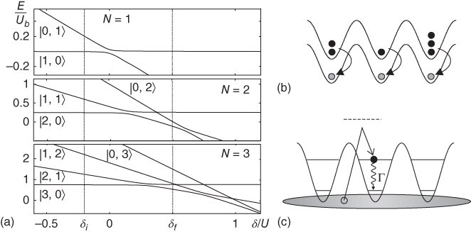
Figure 23.12 (a) Avoided crossings in the energy eigenvalues E for n = 1, 2, 3. (Note the variation in the vertical scale.) For the chosen values of δi and δf (dotted vertical lines), only one avoided crossing is traversed transferring exactly one atom from |a〉 to |b〉 as schematically shown in (b). (c) Loading of an atom into the first Bloch band from a degenerate gas and spontaneous decay to the lowest band via emitting a phonon into the surrounding degenerate gas.
23.3.3.2 Irreversible Loading Schemes
Further improvement could be achieved via irreversible loading schemes. An optical lattice is immersed in an ultracold degenerate gas from which atoms are transferred into the first Bloch band of the lattice. By spontaneous emission of a phonon (39), the atom then decays into the lowest Bloch band as schematically shown in Figure 23.12. By atom–atom repulsion, further atoms are blocked from being loaded into the lattice. This scheme can also be extended to cool atomic patterns in a lattice. In contrast to adiabatic loading schemes, it has the advantage of being repeatable without removing atoms already stored in the lattice.
23.3.4 Quantum Computing in Optical Lattices
The above methods and experiments for creating optical crystals are a very important step toward realizing theoretical ideas for implementing the basic ingredients of a quantum computer. We first discuss how the basic building blocks can be realized, and then turn toward recently developed, more sophisticated setups.
23.3.4.1 Basic Building Blocks of a Quantum Computer
The SF to MI transition is used to initialize the quantum register. In the MI state, each atom has a fixed position and the particle number fluctuations are very small. Using two internal states, each atom can thus be used to realize a qubit. Single‐qubit operations can be realized by laser interactions of atoms and light and controlled entanglement generation is achieved via interactions between atoms trapped in the lattice (31,32,40,41).
23.3.4.2 Single‐Qubit Gates
In principle, it is straightforward to induce single‐qubit gates by using Raman transitions between the two internal states |a〉 and |b〉. Raman transitions with Rabi frequency Ω R and detuning δ are described by the Hamiltonian
which induce rotations of the qubit state on the Bloch sphere. The axis and angle of this rotation depend on the choice of laser parameters and can be chosen freely. The major problem in inducing single qubit operations is addressing of a single atom as it is difficult to focus a laser to spots of order of an optical wave length that is the typical separation between atoms in the lattice. Possible solutions to this difficulty are using schemes for pattern loading (29,42), where only specific lattice sites are filled with atoms or using additional marker atoms that specify the atom the laser is supposed to interact with.
MI atoms in an optical lattice have already experimentally been used as qubits, and it has been shown that they support multiparticle entangled states (43). The robustness of these qubits is, however, limited by stray magnetic fields and spin echo techniques need to be used to perform the experiments successfully. A different approach to obtaining robust quantum memory uses a more sophisticated encoding of the qubits (44). A 1D chain with an even number of atoms encodes a single qubit in the states |0〉 = |abab ⋯ ab〉 and |1〉 = |baba ⋯ ba〉. These states both contain the same number of atoms in internal states |a〉 and |b〉 and therefore interact with magnetic fields in exactly the same way avoiding dephasing of the quantum information stored in the chain. This and the fact that all the atoms have to flip their internal state to get from one logical state to the other make these qubits very robust against the most‐dominant experimental sources of decoherence. However, at the same time, this robustness makes it more difficult to manipulate them. A laser pulse no longer corresponds to a simple rotation on the Bloch sphere spanned by the logical states |0〉 and |1〉 that makes the realization of a single‐qubit gate difficult. We will describe how these problems can be circumvented later and further details can be found in (44).
23.3.4.3 Two‐Qubit Gates
Implementing a two‐qubit gate is more challenging than the single‐qubit gates. The different schemes for two‐qubit gates can be classified in two categories. The first version relies on the concept of a quantum data bus; the qubits are coupled to a collective auxiliary quantum mode, for example, a phonon mode in an ion trap, and entanglement is achieved by swapping the qubits to excitations of the collective mode. The second concept that is the basis for two‐qubit gates between atoms in optical lattices deploys controllable internal‐state dependent two‐body interactions. Examples for different interactions are coherent cold collisions of atoms, optical dipole–dipole interactions (31,32) and the “fast” two‐qubit gate based on large permanent dipole interactions between laser excited Rydberg atoms in static electric fields (40). Besides these dynamical schemes for entanglement creation, it is also possible to generate entanglement by purely geometrical means (45). We will now discuss the different ways to achieve two‐qubit operations in optical lattices.
23.3.4.4 Entanglement via Coherent Ground State Collisions
The interaction terms describing s‐wave collisions between ultracold atoms in one lattice site are analogous to Kerr nonlinearities between photons in quantum optics. For atoms stored in optical lattices these nonlinear atom–atom interactions can be large (31), even for interactions between individual pairs of atoms, thus providing the necessary ingredients to implement two‐qubit gates.
We consider a situation where two atoms in a superposition of internal states |a〉 and |b〉 are trapped in the ground states of two optical lattice sites (see Figure 23.13a). Initially, at time t = −τ, these wells are centered at positions sufficiently far apart so that the particles do not interact. The optical lattice potential is then moved state selectively and for simplicity we assume that only the potential for a particle in internal state |a〉 moves to the right and drags along an atom in state |a〉 while a particle in state |b〉 remains at rest. Thus, the wavefunction of each atom splits up in space according to the internal superposition of states |a〉 and |b〉. When the wavefunction of the left atom in state |a〉 reaches the second atom in state |b〉 as shown in Figure 23.13b, they will interact with each other. However, any other combination of internal states will not interact and therefore this collision is conditional on the internal state. A specific laser configuration achieving this state‐dependent atom transport has been analyzed in Ref. (31) for alkali atoms, based on tuning the laser between the fine structure excited p‐states. The trapping potentials can be moved by changing the laser parameters. Such trapping potentials could also be realized with magnetic and electric microtraps (46).
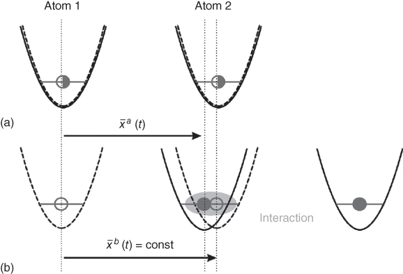
Figure 23.13 We collide one atom in the internal state |a〉 (filled circle, potential indicated by solid curve) with a second atom in state |b〉 (open circle, potential indicated by dashed curve)). In the collision, the wavefunction accumulates a phase according to Eq. 23.25. (a) Configurations at times t = ±τ and (b) at time t.
We therefore only need to consider the situation where atom 1 is in state |a〉 and particle 2 is in state |b〉 to analyze the interactions between the two atoms. The positions of the potentials are moved along the trajectories ![]() and
and ![]() = const
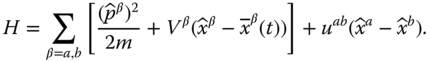
., so that the wavepackets of atoms overlap for a certain time, until they are finally restored to the initial position at the final time t = τ. This situation is described by the Hamiltonian
= const
., so that the wavepackets of atoms overlap for a certain time, until they are finally restored to the initial position at the final time t = τ. This situation is described by the Hamiltonian
Here, ![]() and
and ![]() are the position and momentum operators, Va,b
are the position and momentum operators, Va,b
![]() describe the displaced trap potentials and uab
is the atom–atom interaction term (which leads to the interaction terms in the BHM). Ideally, we want to implement the transformation from before to after the collision,
describe the displaced trap potentials and uab
is the atom–atom interaction term (which leads to the interaction terms in the BHM). Ideally, we want to implement the transformation from before to after the collision,
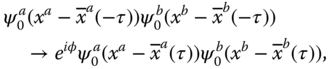
where each atom remains in the ground state ![]() of its trapping potential and preserves its internal state. The phase φ = φa
+ φb
+ φab
will contain a contribution φab
from the interaction (collision) and (trivial) single‐particle kinematic phases φa
and φb
. The transformation Eq. 23.25 can be realized in the adiabatic limit, whereby we move the potentials slowly on the scale given by the trap frequency, so that atoms remain in their motional ground state. In this case, the collisional phase shift is given by φab
=
of its trapping potential and preserves its internal state. The phase φ = φa
+ φb
+ φab
will contain a contribution φab
from the interaction (collision) and (trivial) single‐particle kinematic phases φa
and φb
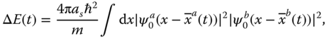
. The transformation Eq. 23.25 can be realized in the adiabatic limit, whereby we move the potentials slowly on the scale given by the trap frequency, so that atoms remain in their motional ground state. In this case, the collisional phase shift is given by φab
= ![]() ΔE(t)/ℏ, where ΔE(t) is the energy shift induced by the atom–atom interactions
ΔE(t)/ℏ, where ΔE(t) is the energy shift induced by the atom–atom interactions
with as the s‐wave scattering length. In addition, we assume that |ΔE(t)| ≪ ℏωT so that no sloshing motion is excited.
The interaction phase thus only applies when atoms are in internal state |a, b〉 but not otherwise. Carrying out the above state‐selective collision with a phase φab = π, we obtain (up to trivial phases) the mapping (as above we identify |a〉 ≡ |0〉 and |b〉 ≡ |1〉)
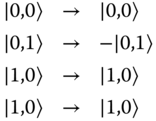
which realizes a two‐qubit phase gate that is universal in combination with single‐qubit rotations.
23.3.4.5 State‐Selective Interaction Potential
An alternative possibility, for a nontrivial logical phase to be obtained, is to rely on a state‐independent trapping potential, while defining a procedure where different logical states couple to each other with different energies. An example is given by the interaction between state‐selectively switched electrical dipoles (40).
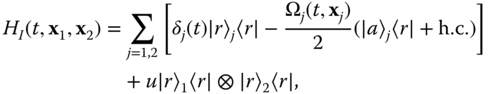
In each qubit, the hyperfine ground states |a〉 ≡ |0〉 is coupled by a laser to a given Stark eigenstate |r〉 that does not correspond to a logical state. The internal dynamics is described by a model Hamiltonian
with Ω
j
(t, x
j
) Rabi frequencies, and δj
(t) detunings of the exciting lasers. Here, u is the dipole–dipole interaction energy between the two particles. We have neglected any loss from the excited states |r〉
j
. We discuss two possible realizations of two‐qubit gates with this dynamics. The most straightforward way to implement a two‐qubit gate is to just switch on the dipole–dipole interaction by exciting each qubit to the auxiliary state |r〉, conditioned on the initial logical state. This can be obtained by two resonant (δ
1 = δ
2 = 0) laser fields of the same intensity, corresponding to a Rabi frequency Ω1 = Ω2 ≫ u. After a time τ = ϕ/u, the gate phase ϕ is accumulated and the particles can be taken again to the initial internal state. However, besides ϕ being sensitive to the atomic distance via the energy shift u, during the gate operation (i.e., when the state |rr〉 is occupied) there are large mechanical effects, due to the dipole–dipole force, which create unwanted entanglement between the internal and the external degrees of freedom. These problems can be overcome by assuming single‐qubit addressability and by moving to the opposite regime of small Rabi frequencies Ω1(t) ≠ Ω2(t) ≪ u. The gate operation is then performed in three steps, by applying: (i) a π‐pulse to the first atom, (ii) a 2π‐pulse (in terms of the unperturbed states) to the second atom, and, finally, (iii) a π‐pulse to the first atom. The state |00〉 is not affected by the laser pulses. If the system is initially in one of the states |01〉 or |10〉, the pulse sequence (i)–(iii) will cause a sign change in the wavefunction. If the system is initially in the state |11〉, the first pulse will bring the system to the state i|r1〉, the second pulse will be detuned from the state |rr〉 by the interaction strength u, and thus accumulate a small phase ![]() ≈ πΩ2/2u ≪ π. The third pulse returns the system to the state
≈ πΩ2/2u ≪ π. The third pulse returns the system to the state ![]() , which realizes a phase gate with ϕ = π −
, which realizes a phase gate with ϕ = π − ![]() ≈ π (up to trivial single‐qubit phases). The time needed to perform the gate operation is of the order τ ≈ 2π/Ω1 + 2π/Ω2. Loss from the excited states |r〉
j
is small provided γΔt ≪ 1, that is, Ω
j
≫ γ. A further improvement is possible by adopting chirped laser pulses with detunings δ
1,2(t) ≡ δ(t) and adiabatic pulses Ω1,2(t) ≡ Ω(t), that is, with a time variation slow on the time scale given by Ω and δ (but still larger than the trap oscillation frequency), so that the system adiabatically follows the dressed states of the Hamiltonian HI
. As found in (40), in this adiabatic scheme the gate phase is
≈ π (up to trivial single‐qubit phases). The time needed to perform the gate operation is of the order τ ≈ 2π/Ω1 + 2π/Ω2. Loss from the excited states |r〉
j
is small provided γΔt ≪ 1, that is, Ω
j
≫ γ. A further improvement is possible by adopting chirped laser pulses with detunings δ
1,2(t) ≡ δ(t) and adiabatic pulses Ω1,2(t) ≡ Ω(t), that is, with a time variation slow on the time scale given by Ω and δ (but still larger than the trap oscillation frequency), so that the system adiabatically follows the dressed states of the Hamiltonian HI
. As found in (40), in this adiabatic scheme the gate phase is
with ![]() = δ − Ω2
/(4δ + 2u) the detuning including a Stark shift. For a specific choice of pulse duration and shape Ω(t) and δ(t), we achieve ϕ(τ) = π. To satisfy the adiabatic condition, the gate operation time τ has to be approximately one order of magnitude longer than in the other scheme discussed above. In the ideal limit Ω
j
≪ u, the dipole–dipole interaction energy shifts the doubly excited state |rr〉 away from resonance. In such a “dipole‐blockade” regime, this state is therefore never populated during gate operation. Hence, the mechanical effects due to atom–atom interaction are greatly suppressed. Furthermore, this version of the gate is only weakly sensitive to the exact distance between atoms, since the distance‐dependent part of the entanglement phase is
= δ − Ω2
/(4δ + 2u) the detuning including a Stark shift. For a specific choice of pulse duration and shape Ω(t) and δ(t), we achieve ϕ(τ) = π. To satisfy the adiabatic condition, the gate operation time τ has to be approximately one order of magnitude longer than in the other scheme discussed above. In the ideal limit Ω
j
≪ u, the dipole–dipole interaction energy shifts the doubly excited state |rr〉 away from resonance. In such a “dipole‐blockade” regime, this state is therefore never populated during gate operation. Hence, the mechanical effects due to atom–atom interaction are greatly suppressed. Furthermore, this version of the gate is only weakly sensitive to the exact distance between atoms, since the distance‐dependent part of the entanglement phase is ![]() ≪ π. For the same reason, possible excitations in the particles' motion do not alter significantly the gate phase, leading to a very weak temperature dependence of the fidelity.
≪ π. For the same reason, possible excitations in the particles' motion do not alter significantly the gate phase, leading to a very weak temperature dependence of the fidelity.
23.3.4.6 Universal Quantum Simulators
Building a general purpose quantum computer, which is able to run, for example, Shor's algorithm, requires quantum resources that will only be available in the long term future. Thus, it is important to identify nontrivial applications for quantum computers with limited resources, which are available in the lab at present. Such an example is provided by Feynman's universal quantum simulator (UQS) (47). A UQS is a controlled device that, operating itself on the quantum level, efficiently reproduces the dynamics of any other many‐particle system that evolves according to short‐range interactions. Consequently, a UQS could be used to efficiently simulate the dynamics of a generic many‐body system, and in this way function as a fundamental tool for research in many‐body physics, for example, to simulate spin systems.
According to Jane et al. (48), the very nature of the Hamiltonian available in quantum optical systems makes them best suited for simulating the evolution of systems whose building blocks are also two‐level atoms, and having a Hamiltonian HN
= ∑
a H
(a) + ∑
a≠b
H(ab) that decomposes into one‐qubit terms H
(a) and two‐qubit terms H
(ab). A starting observation concerning the simulation of quantum dynamics is that if a Hamiltonian ![]() decomposes into terms Kj
acting in a small constant subspace, then by the Trotter formula e−iKτ
= lim
m→∞
decomposes into terms Kj
acting in a small constant subspace, then by the Trotter formula e−iKτ
= lim
m→∞
![]() , we can approximate an evolution according to K by a series of short evolutions according to the pieces Kj
. Therefore, we can simulate the evolution of an N‐qubit system according to the Hamiltonian HN
by composing short one‐qubit and two‐qubit evolutions generated, respectively, by H
(a) and H
(ab). In quantum optics, an evolution according to one‐qubit Hamiltonians H
(a) can be obtained directly by properly shining a laser beam on atoms or ions that host the qubits. Instead, two‐qubit Hamiltonians are achieved by processing some given interaction
, we can approximate an evolution according to K by a series of short evolutions according to the pieces Kj
. Therefore, we can simulate the evolution of an N‐qubit system according to the Hamiltonian HN
by composing short one‐qubit and two‐qubit evolutions generated, respectively, by H
(a) and H
(ab). In quantum optics, an evolution according to one‐qubit Hamiltonians H
(a) can be obtained directly by properly shining a laser beam on atoms or ions that host the qubits. Instead, two‐qubit Hamiltonians are achieved by processing some given interaction ![]() (see the example below) that is externally enforced in the following way. Let us consider two of the N qubits, that we denote by a and b. By alternating evolutions according to some available, switchable two‐qubit interaction
(see the example below) that is externally enforced in the following way. Let us consider two of the N qubits, that we denote by a and b. By alternating evolutions according to some available, switchable two‐qubit interaction ![]() for some time with local unitary transformations, one can achieve an evolution
for some time with local unitary transformations, one can achieve an evolution
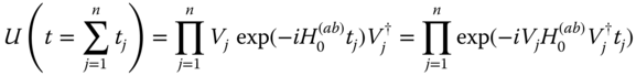
where ![]() with uj
and vj
being one‐qubit unitaries. For a small time interval U(t) ≃ 1 − it
with uj
and vj
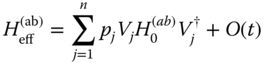
being one‐qubit unitaries. For a small time interval U(t) ≃ 1 − it ![]() with pj
= tj
/t, so that by concatenating several short gates U(t), U(t) = exp
with pj
= tj
/t, so that by concatenating several short gates U(t), U(t) = exp ![]() + O(t
2),we can simulate the Hamiltonian
+ O(t
2),we can simulate the Hamiltonian
for larger times. Note that the systems can be classified according to the availability of homogeneous manipulation, uj = vj , or the availability of local individual addressing of the qubits, uj ≠ vj .
Cold atoms in optical lattices provide an example where single atoms can be loaded with high fidelity into each lattice site, and where cold‐controlled collisions provide a way of entangling these atoms in a highly parallel way. This assumes that atoms have two internal (ground) states |0〉 ≡ |↓〉 and |1〉 ≡ |↑〉 representing a qubit, and that we have two spin‐dependent lattices, one trapping the |0〉 state, and the second supporting the |1〉 state. An interaction between adjacent qubits is achieved by displacing one of the lattices with respect to the other as discussed in the previous subsection. In this way, the |0〉 component of the atom a approaches in space the |1〉 component of the atom a + 1, and these collide in a controlled way. Then, the two components of each atom are brought back together. This provides an example of implementing an Ising ∑
a≠b
![]() = ∑
a
= ∑
a
![]() ⊗ σz
(a+1) interaction between the qubits, where the σ
(a)′s denote Pauli matrices. By a sufficiently large, relative displacement of the two lattices, also interactions between more distant qubits could be achieved. A local unitary transformation can be enforced by shining a laser on the atoms, inducing an arbitrary rotation between |0〉 and |1〉. On the time scale of the collisions requiring a displacement of the lattice (the entanglement operation), these local operations can be assumed instantaneous. In the optical lattice example, it is difficult to achieve an individual addressing of the qubits. Such an addressing would be available in an ion‐trap array as discussed in Ref. (49). These operations provide us with the building blocks to obtain an effective Hamiltonian evolution by time averaging as outlined above.
⊗ σz
(a+1) interaction between the qubits, where the σ
(a)′s denote Pauli matrices. By a sufficiently large, relative displacement of the two lattices, also interactions between more distant qubits could be achieved. A local unitary transformation can be enforced by shining a laser on the atoms, inducing an arbitrary rotation between |0〉 and |1〉. On the time scale of the collisions requiring a displacement of the lattice (the entanglement operation), these local operations can be assumed instantaneous. In the optical lattice example, it is difficult to achieve an individual addressing of the qubits. Such an addressing would be available in an ion‐trap array as discussed in Ref. (49). These operations provide us with the building blocks to obtain an effective Hamiltonian evolution by time averaging as outlined above.
As an example, let us consider the ferromagnetic [antiferromagnetic] Heisenberg Hamiltonian
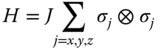
where J > 0 [J < 0]. An evolution can be simulated by short gates with ![]() = γσz
⊗ σz
alternated with local unitary operations
= γσz
⊗ σz
alternated with local unitary operations
without local addressing, as provided by the standard optical lattice setup. The ability to perform independent operations on each of the qubits would translate into the possibility to simulate any bipartite Hamiltonians.
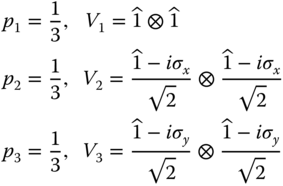
An interesting aspect is the possibility to simulate effectively different lattice configurations: for example, in a 2D pattern a system with nearest neighbor interactions in a triangular configuration can be obtained from a rectangular array configuration. This is achieved by making the subsystems in the rectangular array interact not only with their nearest neighbor but also with two of their next‐to‐nearest neighbors in the same diagonal (see Figure 23.14).
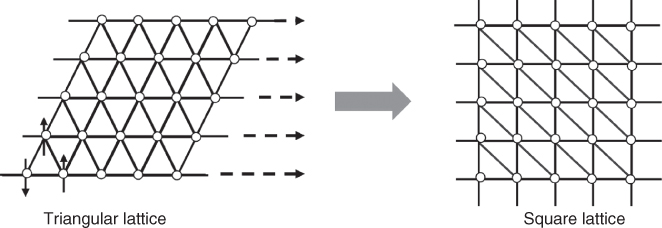
Figure 23.14 Illustrating how triangular configurations of atoms with nearest neighbor interactions may be simulated in a rectangular lattice.
One of the first and most interesting applications of quantum simulations is the study of quantum phase transitions (50). In this case, one would obtain the ground state of a system, adiabatically connecting ground states of systems in different regimes of coupling parameters, allowing to determine its properties.
23.3.4.7 Multiparticle Maximally Entangled States in Optical Lattices
Let us assume that the Rydberg interactions between neighboring atoms are turned on all the time and that atoms are arranged in a 1D chain. Furthermore, we allow each atom to either tunnel between two adjacent wells whose ground states are denoted by |a〉 and |b〉 or to have an additional laser driving Raman transitions between two internal states (again denoted by |a〉 and |b〉). This situation is schematically shown in Figure 23.15.
Figure 23.15 Creation of robust multiparticle entangled states in 1D beam splitter setups. Closed circles indicate an atom; open circles an empty position.
The dynamics of this setup can be understood as follows. Hopping between the two modes |a〉 j and |b〉 j of the jth atom is described by
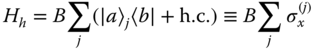
with ![]() the Pauli x‐matrix for the two states (viewed as a spin) of the jth atom and B > 0 the energy associated with this process. The ground state of this Hamiltonian is obtained by putting each atom into an equal superposition of states written in spin notation as |↓x
〉
j
= (|↑z
〉 − |↓z
〉)/
the Pauli x‐matrix for the two states (viewed as a spin) of the jth atom and B > 0 the energy associated with this process. The ground state of this Hamiltonian is obtained by putting each atom into an equal superposition of states written in spin notation as |↓x
〉
j
= (|↑z
〉 − |↓z
〉)/![]() , where |↑z
〉 ≡ |a〉 and |↓z
〉 ≡ |b〉, that is, we find
, where |↑z
〉 ≡ |a〉 and |↓z
〉 ≡ |b〉, that is, we find
Note that this part of the Hamiltonian is identical to a spin chain in a magnetic field B along the x‐axis.
The interaction between two nearest neighbors due to Rydberg interactions is given by
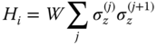
accounting for the energy difference of having two adjacent particles in the same vs. different internal states. In this case, the ground state depends on the sign of the interaction parameter W. For repulsive interactions W > 0, the interaction will be minimized by arranging the particles as
while for attractive interactions the ground state is
Both of these states are maximally entangled multiparticle states, that is, extensions of the well‐known GHz states for three particles.
In the total Hamiltonian H = Hh + Hi , the interaction energy and the hopping energy compete with each other resulting in a quantum phase transition. When the interaction energy is kept constant and the hopping term is switched off adiabatically, as shown in Figure 23.15, the state of the system will dynamically change from |Ψ h 〉, which is a product state to one of the two states |Ψ ir 〉 or |Ψ ia 〉 depending on the sign of the interaction. The exact values of the parameters α and β depend on the details of the dynamics and are discussed in (44). These maximally entangled states can serve different purposes depending on the sign of W. Let us discuss the possible applications of these two kinds of maximally entangled states.
23.3.4.8 Repulsive Interactions
In this case, both parts of the superposition state have the same number of particles in each of the two internal states and thus external stray fields act identically on both, therefore not affecting the parameters α and β. Because of this stability, one can use them for storing quantum information in a robust way. Single‐qubit gates can be performed by dynamically going back and forth through the quantum phase transition in the whole chain changing the parameters α and β in a controlled way.
23.3.4.9 Attractive Interactions
For attractive interactions, the terms in the superposition of |ψia 〉 will respond to external fields very differently. Therefore, the relative phase between the parameters α and β will be very susceptible to these fields, in fact for N particles in the chain, this phase will be N times larger than if there was just a single particle. The two parts of |ψia 〉 can thus be used as two arms of an entanglement enhanced atomic interferometer.
23.3.4.10 A Single‐Atom Transistor in a 1D Optical Lattice
As a second example, we consider a spin‐1/2 atomic impurity that is used to switch the transport of either a 1D BEC or a 1D degenerate Fermi gas initially situated to one side of the impurity (51). In one spin state, the impurity is transparent to the probe atoms, while in the other, it acts as single atom mirror prohibiting transport. Observation of the atomic current passing the impurity can then be used as a quantum nondemolition measurement of its internal state, which can be seen to encode a qubit, |ψq 〉 = α|↑〉 + β|↓〉. If a macroscopic number of atoms pass the impurity, then the system will be in a macroscopic superposition, |ψ(t)〉 = α|↑〉|φ↑ (t)〉 + β|↓〉|φ↓ (t)〉, which can form the basis for a single‐shot readout of the qubit spin. Here, |φσ (t)〉 denotes the state of the probe atoms after evolution to time t, given that the qubit is in state σ (see Figure 23.16). In view of the analogy between state amplification via this type of blocking mechanism and readout with single‐electron transistors (SET) used in solid‐state systems, we refer to this setup as a single‐atom transistor (SAT).
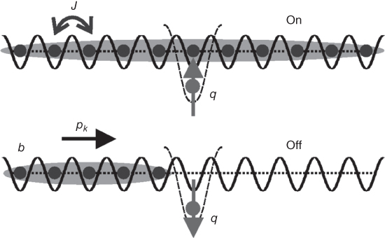
Figure 23.16 A spin 1/2 impurity q used as a switch: in one spin state it is transparent to the probe atoms “on,” but in the other it acts as a single atom mirror “off.” Probe atoms b approaching with momentum pk are either transmitted or reflected at the impurity.
We consider the implementation of a SAT using cold atoms in 1D optical lattices: probe atoms in the state |b〉 are loaded in the lattice to the left of a site containing the impurity atom |q〉, which is trapped by a separate (e.g., spin dependent) potential (cf. Figure 23.16). The passage of |b〉 atoms past the impurity q is then governed by the spin‐dependent effective collisional interaction ![]() . By making use of a quantum interference mechanism, we engineer complete blocking (effectively U
eff → ∞) for one spin state and complete transmission (U
eff → 0) for the other.
. By making use of a quantum interference mechanism, we engineer complete blocking (effectively U
eff → ∞) for one spin state and complete transmission (U
eff → 0) for the other.
The quantum interference mechanism needed to engineer U
eff can be produced using an optical or a magnetic Feshbach resonance (52–54), and we use the present example to illustrate Hamiltonians for impurity interactions involving Feshbach resonances and molecular interactions. For the optical case, a Raman laser drives a transition on the impurity site, 0, from the atomic state ![]() via an off‐resonant excited molecular state to a bound molecular state back in the lowest electronic manifold
via an off‐resonant excited molecular state to a bound molecular state back in the lowest electronic manifold ![]() (Figure 23.17a). We denote the effective two‐photon Rabi frequency and detuning by Ω
σ
and Δ
σ
, respectively. The Hamiltonian for our system is then given by Ĥ = Ĥb
+ Ĥ
0, with
(Figure 23.17a). We denote the effective two‐photon Rabi frequency and detuning by Ω
σ
and Δ
σ
, respectively. The Hamiltonian for our system is then given by Ĥ = Ĥb
+ Ĥ
0, with
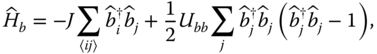
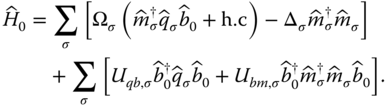
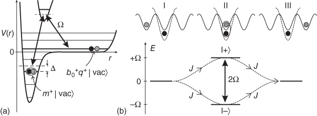
Figure 23.17
(a) The optical Feshbach setup couples the atomic state  (in a particular motional state quantized by the trap) to a molecular bound state of the Born–Oppenheimer potential,
  , with the effective Rabi frequency Ω
σ
and detuning Δ
σ
. (b) A single atom passes the impurity (I → III) via the two dressed states (II), |+〉 =
, with the effective Rabi frequency Ω
σ
and detuning Δ
σ
. (b) A single atom passes the impurity (I → III) via the two dressed states (II), |+〉 =  〉 +
〉 +  and |−〉 =
 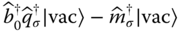 . Quantum interference between the paths gives rise to an effective tunneling rate J
eff,σ
.
. Quantum interference between the paths gives rise to an effective tunneling rate J
eff,σ
.
Here Ĥ b is a familiar Hubbard Hamiltonian for atoms in the state |b〉; Ĥ 0 describes the additional dynamics due to the impurity on site 0, where atoms in the state |b〉 and |q〉 are converted to a molecular state with effective Rabi frequency Ω σ and detuning Δ σ , and the last two terms describe background interactions, Uαβ,σ for two particles α, β ∈ {qσ , b, m}, which are typically weak. This model is valid for Uαβ, J, Ω, Δ ≪ ω T (where ω T is the energy separation between Bloch bands). Because the dynamics for the two spin channels qσ can be treated independently, in the following we will consider a single spin channel, and drop the subscript σ.
To understand the qualitative physics behind the above Hamiltonian, let us consider the molecular couplings and associated effective interactions between the |q〉 and |b〉 atoms for (i) off‐resonant (Ω ≪ |Δ|) and (ii) resonant (Δ = 0) laser driving. In the first case, the effective interaction between |b〉 and |q〉 atoms is U
eff = Uqb
+ Ω2
/Δ, where the second term is an AC‐Stark shift that plays the role of the resonant enhancement of the collisional interactions between |b〉 and |q〉 atoms due to the optical Feshbach resonance. For resonant driving (Δ = 0), the physical mechanism changes. On the impurity site, laser driving mixes the states ![]() and m
†
|vac〉, forming two dressed states with energies ε±
= (Uqb
)/2 ± (
and m
†
|vac〉, forming two dressed states with energies ε±
= (Uqb
)/2 ± (![]() /4 + Ω2)1/2 (Figure 23.17b, II). Thus, we have two interfering quantum paths via the two dressed states for the transport of |b〉 atoms past the impurity. In the simple case of weak tunneling Ω ≫ J and Uqb
= 0 second‐order perturbation theory gives for the effective tunneling
/4 + Ω2)1/2 (Figure 23.17b, II). Thus, we have two interfering quantum paths via the two dressed states for the transport of |b〉 atoms past the impurity. In the simple case of weak tunneling Ω ≫ J and Uqb
= 0 second‐order perturbation theory gives for the effective tunneling ![]() (|ε| ≪ Ω) that shows destructive quantum interference, analogous to the interference effect underlying electromagnetically induced transparency (EIT) (55), and is equivalent to having an effective interaction U
eff → ∞.
(|ε| ≪ Ω) that shows destructive quantum interference, analogous to the interference effect underlying electromagnetically induced transparency (EIT) (55), and is equivalent to having an effective interaction U
eff → ∞.
In Ref. (51) the exact dynamics for scattering of a single |b〉 atom from the impurity is solved exactly, confirming the above qualitative picture of EIT‐type quantum interference. Furthermore, in this reference, a detailed study of the time‐dependent many‐body dynamics based on the 1D Hamiltonian (23.38) is presented for interacting many‐particle systems including a 1D Tonks gas.
References
- 1 Cirac, J.I. and Zoller, P. (1995) Phys. Rev. Lett., 74, 4091–4094.
- 2 Steane, A. (1997) App. Phys. B, 64, 623.
- 3 Cirac, J.I., Duan, L.M., Jaksch, D., and Zoller, P. (2002) Quantum optical implementation of quantum information processing, in Proceedings of the International School of Physics “Enrico Fermi” Course CXLVIII, Experimental Quantum Computation and Information (eds F. De Martini and C. Monroe), IOS Press, Amsterdam.
- 4 Zoller, P., Cirac, J.I., Duan, L., and García‐Ripoll, J.J. (2004) Quantum entanglement and information processing, in Proceedings of the Les Houches Summer School, Session 79 (eds D. Estève, J.M. Raimond, and J. Dalibard), Elsevier, Amsterdam.
- 5 Poyatos, J.F., Cirac, J.I., and Zoler, P. (1998) Phys. Rev. Lett., 81 (6), 1322–1325.
- 6 Molmer, K. and Sorensen, A. (1999) Phys. Rev. Lett., 82 (9), 1835–1838.
- 7 Sorensen, A. and Molmer, K. (1999) Phys. Rev. Lett., 82 (9), 1971–1974.
- 8 Milburn, G.J., Schneider, S., and James, D.F.V. (2000) Fortschr. Phys., 48, 9–11.
- 9 García‐Ripoll, J.J., Zoller, P., and Cirac, J.I. (2003) Phys. Rev. Lett., 91, 157901.
- 10 García‐Ripoll, J.J., Zoller, P., and Cirac, J.I. (2005) Phys. Rev. A, 71, 062309.
- 11 Duan, L.‐M., Cirac, J.I., and Zoller, P. (2001) Science, 292, 1695–1697.
- 12 Gardiner, C.W. and Zoller, P. (1999) Quantum Noise, chapter, Springer, Berlin.
- 13 DeMarco, B., Ben‐KIsh, A., Leibfried, D., Meyer, V., Rowe, M., Jelenkovic, B.M., Itano, W.M., Briton, J., Langer, C., Rosenband, T., and Wineland, D.J. (2002) Phys. Rev. Lett., 89 (26), 267901.
- 14 Leibfried, D., DeMarco, B., Meyer, V., Lucas, D., Barret, M., Britton, J., Itano, W.M., Jelenkovic, B., Langer, C., Rosenband, T., and Wineland, D.J. (2003) Nature, 422, 412.
- 15 Schmidt‐Kaler, F., Häffner, H., Riebe, M., Gulde, S., Lancaster, G.P.T., Deuschle, T., Becher, C., Roos, C.F., Eschner, J., and Blatt, R. (2003) Nature, 422, 408–411.
- 16 Cirac, J.I. and Zoler, P. (2000) Nature, 404 (6), 579–581.
- 17 Kielpinski, D., Monroe, C., and Wineland, D.J. (2002) Nature, 417 (13), 709–711.
- 18 Tian, L. and Zoller, P. (2003) Phys. Rev. A, 68, 042321.
- 19 Stenholm, S. (1986) Rev. Mod. Phys., 58, 699–739.
- 20 Wineland, D.J., Monroe, C., Itano, W.M., Leibfried, D., King, B.E., and Meekhof, D.M. (1998) J. Res. Nat. Inst. Stand. Technol., 103, 259.
- 21 King, B.E., Wood, C.S., Myatt, C.J., Turchette, Q.A., Leibfried, D., Itano, W.M., Monroe, C., and Wineland, D.J. (1998) Phys. Rev. Lett., 81, 1525–1528.
- 22 Roos, C.F., Leibfried, D., Mundt, A., Schmidt‐Kaler, F., Eschner, J., and Blatt, R. (2000) Phys. Rev. Lett., 85, 5547–5550.
- 23 Calarco, T., Cirac, J.I., and Zoller, P. (2001) Phys. Rev. A, 63, 062304.
- 24 Jonathan, D., Plenio, M.B., and Knight, P.L. (2000) Phys. Rev. A, 62, 042307.
- 25 (a) Anderson, B.P. and Kasevich, M.A. (1998) Science, 282, 1686; (b) Orzel, C., Tuchman, A.K., Fenselau, M.L., Yasuda, M., and Kasevich, M.A. (2001) Science, 291, 2386.
- 26 Hensinger, W.K., Häffner, H., Browaeys, A., Heckenberg, N.R., Helmerson, K., McKenzie, C., Milburn, G.J., Phillips, W.D., Rolston, S.L., Rubinsztein‐Dunlop, H., and Upcroft, B. (2001) Nature, 412, 52.
- 27 Greiner, M., Mandel, O., Esslinger, T., Haensch, T.W., and Bloch, I. (2002) Nature, 415, 39.
- 28 Jessen, P.S. and Deutsch, I.H. (1996) Adv. At. Mol. Opt. Phys., 37, 95–138410, 1996.
- 29 Jaksch, D., Bruder, C., Cirac, J.I., Gardiner, C.W., and Zoller, P. (1998) Phys. Rev. Lett., 81, 3108.
- 30 Kohn, W. (1959) Phys. Rev., 115, 809.
- 31 Jaksch, D., Briegel, H., Cirac, J., Gardiner, C., and Zoller, P. (1975) Phys. Rev. Lett., 82, 1999.
- 32 Brennen, G.K., Caves, C.M., Jessen, P.S., and Deutsch, I.H. (1999) Phys. Rev. Lett., 82, 1060.
- 33 Liu, W., Wilczek, F., and Zoller, P. (2004) Phys. Rev. A, 70, 033603.
- 34 Fisher, M., Weichman, P., Grinstein, G., and Fisher, D. (1989) Phys. Rev. B, 40, 546.
- 35 Hofstetter, W., Cirac, J.I., Zoller, P., Demler, E., and Lukin, M. (2002) Phys. Rev. Lett., 89, 220407.
- 36 Stöferle, T., Moritz, H., Schori, C., Köhl, M., and Esslinger, T. (2004) Phys. Rev. Lett., 92, 130403.
- 37 Peil, S., Porto, J., Tolra, B.L., Obrecht, J., King, B., Subbotin, M., Rolston, S., and Phillips, W. (2003) Phys. Rev. A, 67, 051603.
- 38 Rabl, P., Daley, A.J., Fedichev, P.O., Cirac, J.I., and Zoller, P. (2003) Phys. Rev. Lett., 91, 110403.
- 39 Daley, A.J., Fedichev, P.O., and Zoller, P. (2004) Phys. Rev. A, 69, 022306.
- 40 Jaksch, D., Cirac, J.I., Zoller, P., Rolston, S.L., Cote, R., and Lukin, M.D. (2000) Phys. Rev. Lett., 85, 2208.
- 41 Pachos, J.K. and Knight, P.L. (2003) Phys. Rev. Lett., 91, 107902.
- 42 Peil, S., Porto, J.V., Laburthe Tolra, B., Obrecht, J.M., King, B.E., Subbotin, M., Rolston, S.L., and Phillips, W.D. (2003) Phys. Rev. A, 67, 051603(R).
- 43 Mandel, O. et al. (2003) Nature, 425, 937.
- 44 Dorner, U., Fedichev, P., Jaksch, D., Lewenstein, M., and Zoller, P. (2003) Phys. Rev. Lett., 91, 073601.
- 45 Duan, L.‐M., Cirac, J.I., and Zoller, P. (2001) Science, 292, 1695.
- 46 Calarco, T., Briegel, H.‐J., Jaksch, D., Cirac, J.I., and Zoller, P. (2000) J. Mod. Opt., 47, 2137.
- 47 Lloyd, S. (1996) Science, 273, 1073.
- 48 Jane, E., Vidal, G., Dür, W., Zoller, P., and Cirac, J. (2003) Quantum Inf. Comput., 3 (1), 15–37.
- 49 Cirac, J.I. and Zoller, P. (2004) Phys. Today, 38–44, http://www.physicstoday.org/vol‐57/iss‐3/contents.html.
- 50 Sachdev, S. (1999) Quantum Phase Transitions, Cambridge University Press, Cambridge.
- 51 Micheli, A., Daley, A.J., Jaksch, D., and Zoller, P. (2004) Phys. Rev. Lett., 93, 140408.
- 52 Bolda, E., Tiesinga, E., and Julienne, P. (2002) Phys. Rev. A, 013403.
- 53 Theis, M., Thalhammer, G., Winkler, K., Hellwig, M., Ruff, G., Grimm, R., and Denschlag, J.H. (2004) Phys. Rev. Lett., 93, 123001.
- 54 Calarco, T., Dorner, U., Julienne, P., Williams, C., and Zoller, P. (2004) Phys. Rev. A, 70, 012306.
- 55 Lukin, M. (2003) Rev. Mod. Phys., 75, 457.