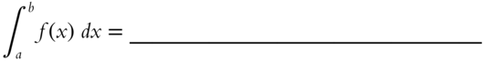
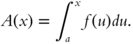
CHAPTER THREE
Integral Calculus
In this chapter you will learn about:
- Antiderivatives and the indefinite integral;
- Integrating a variety of functions;
- Some applications of integral calculus;
- Finding the area under a curve;
- Definite integrals with applications;
- Multiple integrals.
The previous chapter was devoted to the first major branch of calculus—differential calculus. This chapter is devoted to the second major branch—integral calculus. The two branches have different natures: differential calculus has procedures that make it possible to differentiate any continuous function; integral calculus has no such general procedures—every problem presents a fresh puzzle. Nevertheless, integral calculus is essential to all of the sciences, engineering, economics, and in fact to every discipline that deals with quantitative information.
There are two routes to introducing the concepts of integration. Although they start in different directions, they finally meld and create a single entity. If they were marked by road signs, the first would be “Antiderivatives and the indefinite integral” while the second would be “Area under a curve and the definite integral.”
3.1 Antiderivative, Integration, and the Indefinite Integral
306
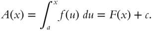
The Antiderivative:
The goal of this section is to learn some techniques for integration, sometimes called antidifferentiation.
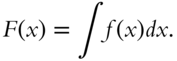
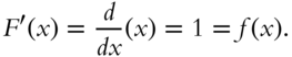
In this section we generally designate a function by ![]() . The concept of the antiderivative is fundamental to the process of integration and is easily explained. When a function
. The concept of the antiderivative is fundamental to the process of integration and is easily explained. When a function ![]() is differentiated to give
is differentiated to give ![]() , then
, then ![]() is an antiderivative of
is an antiderivative of ![]() , that is,
, that is,
This notation describes the defining property of the antiderivative, although only in terms of the derivative ![]() , not
, not ![]() itself.
itself.
The antiderivative is usually written in the form:
The expression ![]() is also called the integral of
is also called the integral of ![]() . The symbol
. The symbol ![]() is known as the integration symbol; it represents the inverse of differentiation.
is known as the integration symbol; it represents the inverse of differentiation.
To summarize the notation, if F′(x) = f(x), then F(x) is the _____________ or _________________________.
Go to 307.
307
Indefinite Integral:
Often one can find the antiderivative simply by guesswork. For instance, if ![]() , then
, then ![]() . To prove this, note that
. To prove this, note that
However, ![]() is not the only antiderivative of
is not the only antiderivative of ![]() ;
; ![]() , where
, where ![]() is a constant, is also an antiderivative because
is a constant, is also an antiderivative because

In fact, a constant can always be added to a function without changing its derivative. If ![]() is an antiderivative of
is an antiderivative of ![]() , then all the antiderivatives of
, then all the antiderivatives of ![]() can be denoted by writing
can be denoted by writing

where ![]() is an arbitrary constant.
is an arbitrary constant.
If it is useful, we can write the defining equation for the antiderivative in terms of a differential: ![]() . (If you need to review differentials, see frame 264.) Then we can describe all the antiderivatives by the notation
. (If you need to review differentials, see frame 264.) Then we can describe all the antiderivatives by the notation
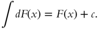
Because of the arbitrary constant, the definition is imprecise. For this reason this integral is called the indefinite integral.
In summary, the integral of the differential of a function is equal to the function plus a constant.
Go to 308.
308
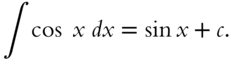
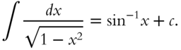
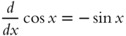
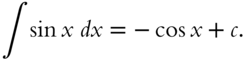
Because this first meaning of integration is the inverse of differentiation, for every differentiation formula in Chapter 2, there is a corresponding integration formula here. Thus from Chapter 2, frame 211,
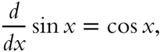
so by the definition of the indefinite integral,
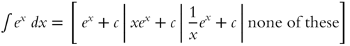
Now you try one. What is ![]() Choose the answer: [cos x + c | −cos x + c | sin x cos x + c | none of these]
Choose the answer: [cos x + c | −cos x + c | sin x cos x + c | none of these]
Make sure you understand the correct answer (you can check the result by differentiation).
Go to 309.
309
Now try to find these integrals:
 ,
,  .
.
If you did both of these correctly, skip to frame 311.
If not, go to frame 310.
310
If you had difficulty with these problems, recall the definition of the indefinite integral. If ![]() then
then ![]()
In order to find ![]() , we must find an expression that when differentiated yields the given function
, we must find an expression that when differentiated yields the given function ![]() . For instance, the derivative of
. For instance, the derivative of ![]() is
is
by the formula for differentiating ![]() in frame 180. Hence,
in frame 180. Hence, ![]() is an integral of
is an integral of ![]() . But the integral is indefinite because we could add any constant to it without changing its defining property:
. But the integral is indefinite because we could add any constant to it without changing its defining property: ![]() . Thus, including the integration constant
. Thus, including the integration constant ![]() , we find
, we find ![]() . (Note that this formula does not work for
. (Note that this formula does not work for ![]() . That case will be discussed later.)
. That case will be discussed later.)
Likewise, by frame 235,
But the integral is indefinite because we could add any constant. Thus
Go to 311.
311
A table with some common integrals is given in the next frame. You can check the truth of any of the equations ![]() by confirming that
by confirming that ![]() We will shortly use this method to verify some of the equations.
We will shortly use this method to verify some of the equations.
Go to 312.
312
Table of Integrals:
The following integral table is a list of antiderivatives of some common functions. The integrals occur in many applications and are worth getting to know. For simplicity, in the integration table the arbitrary integration constants are omitted; ![]() and
and ![]() are constants.
are constants.
Table of Integrals
| 1. | |
| 2. | |
| 3. | |
| 4. |  |
| 5. |  |
| 6. |  |
| 7. | |
| 8. | 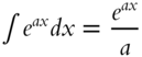 |
| 9. | 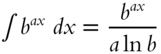 |
| 10. | |
| 11. | |
| 12. | |
| 13. | |
| 14. | |
| 15. | |
| 16. | 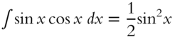 |
| 17. | 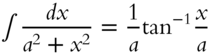 |
| 18. | 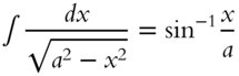 |
| 19. |  |
| 20. | 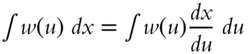 |
| 21. |
For convenience this table is repeated as Table 2: Integrals on page 288.
Go to 313.
313
Let's see if you can check some of the formulas in the table. Show that integral formulas 10 and 16 are correct.
If you have proved the formulas to your satisfaction, go to 315.
If you want to see proofs of the formulas, go to 314.
314
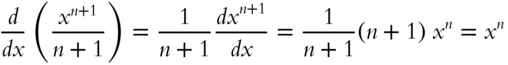
To prove that ![]() , we must show that
, we must show that ![]() .
.
- 10.
 ,
,  .
.

- 16.
 ,
,  .
.

Go to 315.
3.2 Some Techniques of Integration
315
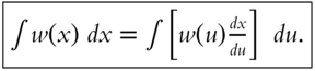
Change of Variable:
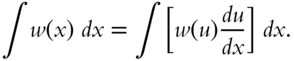
Often an unfamiliar function can be converted into a familiar function having a known integral by using a technique called change of variable. The method applies to integrating a “function of a function.” (Differentiation of such a function was discussed in frame 198. It is differentiated using the chain rule.) For example, ![]() can be written
can be written ![]() , where
, where ![]() . With the following rule, the integral with respect to the variable
. With the following rule, the integral with respect to the variable ![]() can be converted into another integral, often simpler, depending on the variable
can be converted into another integral, often simpler, depending on the variable ![]() .
.
Let's see how this works by applying it to a few problems.
Go to 316.
316
Consider the problem of evaluating the integral

Let ![]() , or
, or ![]() , and
, and ![]() . Hence
. Hence ![]() . Using the rule for change of variable,
. Using the rule for change of variable, 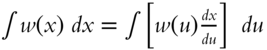 , the integral becomes
To prove that this result is correct, note that
as required.
Try the following somewhat tricky problem. If you need a hint, see frame 317. Evaluate
To check your answer, go to 317.
317
Let ![]() . Then
. Then ![]() , and by the rule for change of variable,
, and by the rule for change of variable,

The integral becomes

Go to 318.
318
Here is an example of a simple change of variable. The problem is to calculate ![]() . If we let
. If we let ![]() , then the integral is
, then the integral is ![]() , which is easy to integrate. Using
, which is easy to integrate. Using ![]() , we have
, we have

To see whether you have caught on, evaluate ![]() (You may find the integral table in frame 312 helpful.)
(You may find the integral table in frame 312 helpful.)

To check your answer, go to 319.
319
Here is the answer:

If you obtained this result, go right on to 320. Otherwise, continue. If we let ![]() , then
, then ![]() and
and

From formula 16 of frame 312 we have

Hence

Let's check this result:

as required. (We have used the chain rule here.)
Go to 320.
320
Try to evaluate ![]() , where a and b are constants. The integral table in frame 312 may be helpful.
, where a and b are constants. The integral table in frame 312 may be helpful.

Go to 321 for the solution.
321
If we let ![]() , then
, then ![]() and
and

Go to 322.
322
We have seen how to evaluate an integral by changing the variable from ![]() to
to ![]() , where
, where ![]() is some constant. Often it is possible to simplify an integral by substituting still other quantities for the variable.
is some constant. Often it is possible to simplify an integral by substituting still other quantities for the variable.
Here is an example. Evaluate:

Suppose we let ![]() . Then
. Then ![]() , and
, and

Try to use this method for evaluating the integral: ![]()
![]()
Go to 323 to check your answer.
323
Taking ![]() , then
, then ![]() and
and

Go to 324.
324
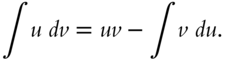
Integration by Parts:
A technique known as integration by parts is sometimes helpful. Let ![]() and
and ![]() be any two functions of
be any two functions of ![]() . Then the rule for integration by parts is
. Then the rule for integration by parts is
Here is the proof: using the product rule for differentiation,

Now integrate both sides of the equation with respect to ![]() .
.

But ![]() , and after transposing, we have
, and after transposing, we have ![]()
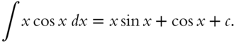
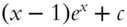
Here is an example: Find ![]() .
.
Let ![]() ,
, ![]() . Then it is easy to see that
. Then it is easy to see that ![]() , and
, and ![]() . Note we have dropped the constant for simplicity. Thus
. Note we have dropped the constant for simplicity. Thus
Go to 325.
325
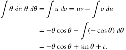
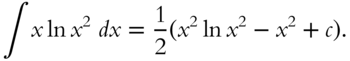
Try to use integration by parts to find ![]() .
.
If right, go to 327.
If you missed this, or want to see how to solve the problem, go to 326.
326
To find ![]() use the formula for integration by parts. Because we now know that
use the formula for integration by parts. Because we now know that ![]() (frame 312, formula 7), we let
(frame 312, formula 7), we let ![]() ,
, ![]() , so that
, so that ![]() ,
, ![]() . Then,
. Then,

Go to 327.
327
Use the method of integration by parts to find the integral: ![]()

Check your answer in 328.
328
Here is the answer:
If you want to see how this is derived, continue here. Otherwise, go on to 329.
Let us make the following substitution ![]() and
and ![]() , and integrate by parts. Thus
, and integrate by parts. Thus ![]() ,
, ![]() , and the integral is
, and the integral is

Go to 329.
329
In integration problems it is often necessary to use a number of different integration “tricks of the trade” in a single problem.
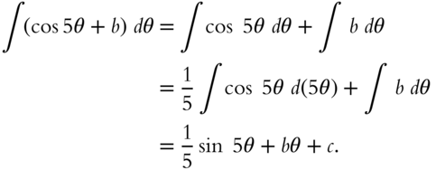
Try the following (b is a constant):
Go to 330 for the answers.
330
The answers are
If you did both of these correctly, you are doing fine—jump ahead to frame 332. If you missed either problem, go to frame 331.
331
If you missed (a), you may have been confused by the change in notation from ![]() to
to ![]() . Remember
. Remember ![]() is merely a symbol for some variable. All the integration formulas could be written replacing the
is merely a symbol for some variable. All the integration formulas could be written replacing the ![]() with
with ![]() or
or ![]() or whatever you wish. Now for (a) in detail:
or whatever you wish. Now for (a) in detail:
For problem (b), let ![]() ,
, ![]() :
:

(The last step uses formula 10, frame 312.) Therefore,
You could also have solved this problem using integration by parts.
Go to 332.
332
Method of Partial Fractions:
A useful manipulation from elementary algebra is to combine two simple fractions into one function. The method of partial fractions involves reversing this process in which you split a function into a sum of fractions with simpler denominators.
To illustrate this method, here is a simple example. Consider the function

Because ![]() , we can write
, we can write
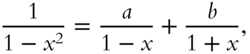
where ![]() and
and ![]() , which are yet to be defined, are called undetermined coefficients. Combining terms yields
, which are yet to be defined, are called undetermined coefficients. Combining terms yields

Equate coefficient of like powers (this is comparable to solving a system of linear equations). Therefore ![]() and
and ![]() . Thus
. Thus ![]() .
.
Now integrate ![]() in terms of simpler integrals that you already know how to evaluate see using formula 6, frame 312.
in terms of simpler integrals that you already know how to evaluate see using formula 6, frame 312.
Go to 333.
333
Now try this problem. Use the method of partial fractions to evaluate the integral ![]() .
.
Go to 334.
334
First note that ![]() . Then write
. Then write

Next, compare coefficients: ![]() and
and ![]() . Solve these two equations with the result that
. Solve these two equations with the result that ![]() . Therefore
. Therefore

Hence the integral is
(The last step uses formula 6, frame 312.)
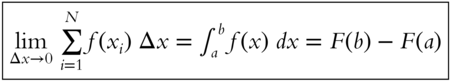
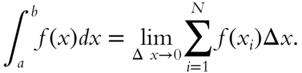
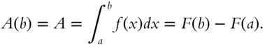
3.3 Area Under a Curve and the Definite Integral
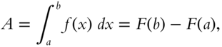
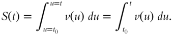
The first section of this chapter focused on the techniques of integration, i.e. finding antiderivatives, all of which are embodied in the term “indefinite integral.” Just as differentiation is useful for many applications besides finding slopes of curves—for instance, calculating rates of growth or finding maxima and minima—so integral calculus has many applications such as finding the volumes of solids or finding the distance traveled by a body moving with a velocity ![]() . These applications all rely on the second type of integration, called the definite integral. This originated in the geometric problem of finding the area under a curve. We start by explaining what “area under a curve” means.
. These applications all rely on the second type of integration, called the definite integral. This originated in the geometric problem of finding the area under a curve. We start by explaining what “area under a curve” means.
Go to 335.
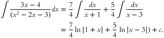
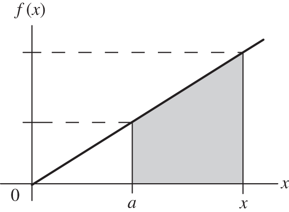
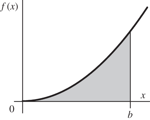
335
Area under a Curve:
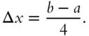
To illustrate what is meant by “the area under a curve,” here is a graph of the simplest of all curves—a straight line given by ![]() .
.
What is the area ![]() between the line
between the line ![]() , and the
, and the ![]() ‐axis between the interval
‐axis between the interval ![]() and
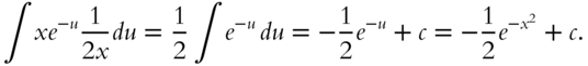
and ![]() ?
?
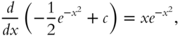
To check your answer, go to 336.
336
The area in the rectangle is the product of the base, ![]() , and the height, 3. Thus the area is
, and the height, 3. Thus the area is ![]() .
.
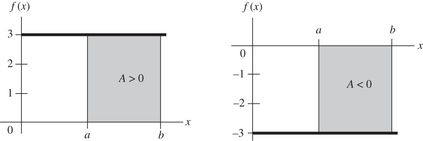
There is an important convention in the sign of the area. In the drawing at the left, because ![]() is positive, the area is positive. However, the area under the graph at the right is negative because the height is
is positive, the area is positive. However, the area under the graph at the right is negative because the height is ![]() , which is negative. Thus, areas can be positive or negative.
, which is negative. Thus, areas can be positive or negative.
Go to 337.
337
A key operation in integral calculus is to find the area under the graph of an arbitrary function ![]() bordered by the
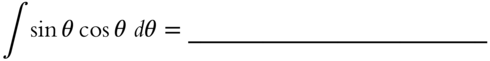
bordered by the ![]() ‐axis between
‐axis between ![]() and
and ![]() , and
, and ![]() and
and ![]() . Our procedure will be to divide the interval
. Our procedure will be to divide the interval ![]() into
into ![]() slices of width
slices of width ![]() , and then watch what happens as
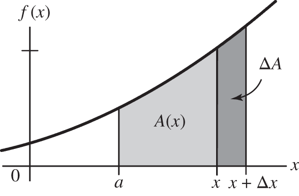
, and then watch what happens as ![]() increases and the width decreases.
increases and the width decreases.
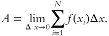
Let's approximate the area under a curve shown in the figure below left using the above procedure.

First we divide the area into a number of strips of equal widths by drawing lines parallel to the vertical axis. The figure shows four such strips. Each strip has an irregular top: but we can divide each strip's area into two sections: a rectangular shape and an approximately triangular shape. Suppose we label the strips 1, 2, 3, 4. The width of each strip is
The height of the first rectangular shape is ![]() , where
, where ![]() is the value of
is the value of ![]() at the beginning of the first strip. Similarly, the height of the second rectangular shape is
at the beginning of the first strip. Similarly, the height of the second rectangular shape is ![]() where
where ![]() . The third and fourth rectangular shapes have heights
. The third and fourth rectangular shapes have heights ![]() and
and ![]() , respectively, where
, respectively, where ![]() and
and ![]() .
.
The height of the first triangular shape is ![]() , where
, where ![]() is the slope of
is the slope of ![]() evaluated at
evaluated at ![]() . The heights of the other triangles are similarly described.
. The heights of the other triangles are similarly described.
You should be able to write an approximate expression for the area of any of the strips. Below write the approximate expression for the area of strip number 3, ΔA3,
The symbol ≈ means “approximately equal to.”
For the correct answer, go to 338.
338
The area of rectangular shape in strip number 3 is ![]() . The triangular shape has area
. The triangular shape has area ![]() . The approximate area of strip 3 is then
. The approximate area of strip 3 is then
Now try to write an approximate expression for A, the total area of all four strips.
Try this, and then see 339 for the correct answer.
339
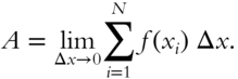
An approximate expression for the total area is simply the sum of the areas of all the strips. In symbols, because A = ΔA1 + ΔA2 + ΔA3 + ΔA4, we have

We could also write this as

∑ is the Greek letter Sigma, which corresponds to the English letter S and stands here for the sum. The symbol  means
means
where ![]() is an index and the counting goes from
is an index and the counting goes from ![]() to
to ![]() .
.
Go to 340.
340
Suppose we divide the area into more strips each of which is narrower, as shown in the drawings. Evidently our approximation gets better and better.

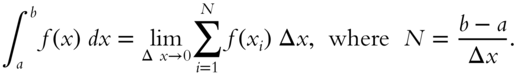
If we divide the area into N strips, then
where ![]() . Now, if we take the limit where Δx → 0, the approximation becomes an equality. Thus,
. Now, if we take the limit where Δx → 0, the approximation becomes an equality. Thus,
Such a limit is so important that it is given a special name and symbol. It is called the definite integral and is written ![]() . This expression looks similar to the antiderivative
. This expression looks similar to the antiderivative ![]() , from frame 327, and as we shall see in the next frame, it is related. However, it is important to remember that the definite integral is defined by the limit described above:
, from frame 327, and as we shall see in the next frame, it is related. However, it is important to remember that the definite integral is defined by the limit described above:

(Incidentally, the integral symbol ![]() also evolved from the letter S and, like sigma, it was chosen to stand for sum.)
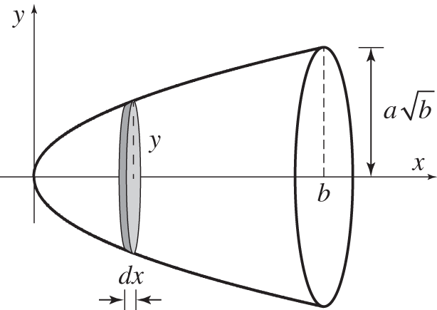
also evolved from the letter S and, like sigma, it was chosen to stand for sum.)
Go to 341.
341
With this definition for the definite integral, the discussion in the last frame shows that the area ![]() under the curve between
under the curve between ![]() and
and ![]() is equal to the definite integral.
is equal to the definite integral.

The function ![]() is called the integrand. The points
is called the integrand. The points ![]() and
and ![]() are called the limits of the integral. This usage has nothing to do with
are called the limits of the integral. This usage has nothing to do with ![]() ; here “limit” simply means the boundary.
; here “limit” simply means the boundary.

The process of evaluating ![]() is often spoken of as “integrating
is often spoken of as “integrating ![]() from
from ![]() to
to ![]() ,” and the expression is called the “integral of
,” and the expression is called the “integral of ![]() from
from ![]() to
to ![]() .” Caution: the indefinite and definite integral both employ the integral symbol
.” Caution: the indefinite and definite integral both employ the integral symbol ![]() , and so they can easily be confused. They are entirely different: the definite integral is a number and is equal to the area under the curve between limits a and b. In contrast the indefinite integral is a function — the antiderivative of the integrand.
, and so they can easily be confused. They are entirely different: the definite integral is a number and is equal to the area under the curve between limits a and b. In contrast the indefinite integral is a function — the antiderivative of the integrand.
Go to 342.
342
The Area Function:
For a given function ![]() , we can introduce a new area function
, we can introduce a new area function ![]() by introducing a variable
by introducing a variable ![]() for the upper limit of the definite integral in frame 341, and to avoid confusion we are renaming the integration variable
for the upper limit of the definite integral in frame 341, and to avoid confusion we are renaming the integration variable ![]()
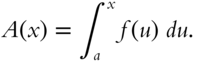
The area function ![]() and the function
and the function ![]() are closely related; the derivative of the area is simply
are closely related; the derivative of the area is simply ![]() . Hence
. Hence
Recall from frame 306 that this means that ![]() is an antiderivative of the function
is an antiderivative of the function ![]() as we will now show.
as we will now show.
Go to 343.
343
To illustrate that ![]() let's look at some simple areas that one can calculate directly.
let's look at some simple areas that one can calculate directly.

The area under the curve ![]() , where
, where ![]() is a constant, is
is a constant, is ![]() Differentiating,
Differentiating, ![]()
Find the area ![]() under
under ![]() between
between ![]() and
and ![]() .
.
Prove to yourself that ![]()
If you want to check your result, go to 344.
Otherwise, skip to 345.
344
One way to calculate the area above is to think of it as the difference of the area of two right triangles. Using area = ½ base × height, we have
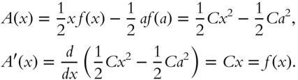
Go to 345.
345
To see why ![]() , consider how the area
, consider how the area ![]() changes as
changes as ![]() increases by an amount
increases by an amount ![]() .
. ![]() , where
, where ![]() is the narrow strip shown.
is the narrow strip shown.
Can you find an approximate expression for ΔA?
This represents a major step in the development of integral calculus, so don't be disappointed if the result eludes you.
Go to 346.
346
The answer we want is
If you wrote this, go on to 347. If you would like a more detailed discussion, read on.
The following argument may appear similar to our definition of the definite integral (frame 340), but here we are proving that the area function is an antiderivative.
Let's take a close look at the area ![]() . As you can see, the area is a long narrow strip, which we divided into a rectangle and a triangle with a small piece remaining. In the figure above we just show the rectangle and triangle. As before (frame 338) the area of the strip is then
. As you can see, the area is a long narrow strip, which we divided into a rectangle and a triangle with a small piece remaining. In the figure above we just show the rectangle and triangle. As before (frame 338) the area of the strip is then
where the small term in the above expression represents the part of the area not included in the triangle or rectangle. For a sufficiently small value of ![]() , the two last terms can be ignored compared to the first term. Therefore in the limit as
, the two last terms can be ignored compared to the first term. Therefore in the limit as ![]()

This supports the conjecture in frame 342 that the area function is an antiderivative, ![]()
Go to 347.
347
To summarize this section, we have found an expression for the area ![]() under a curve defined by
under a curve defined by ![]() that satisfies the equation
that satisfies the equation ![]() Thus, if we can find a function whose derivative is
Thus, if we can find a function whose derivative is ![]() , we can find the area
, we can find the area ![]() up to a constant that remains to be determined to find the exact area.
up to a constant that remains to be determined to find the exact area.
Go to 348.
348
The second meaning of integration, the definite integral, was introduced by the problem of finding the area ![]() under a curve,
under a curve, ![]() , from
, from ![]() to
to ![]() ; this involved finding the limit of an infinite sum. (Recall that this area is a number and not a function.)
; this involved finding the limit of an infinite sum. (Recall that this area is a number and not a function.)
Finding the limit of an infinite sum requires a tedious calculation. Fortunately, we can calculate a definite integral by a far simpler method using the techniques of integration for indefinite integrals. The result is that the area is
where ![]() is any antiderivative of
is any antiderivative of ![]() , i.e.
, i.e. ![]() . What makes this possible is explicitly calculating the constant
. What makes this possible is explicitly calculating the constant ![]() . Instead of calculating a limit, we are now evaluating an antiderivative at the endpoints of the interval.
. Instead of calculating a limit, we are now evaluating an antiderivative at the endpoints of the interval.
Let's begin with the area function associated with a function ![]() from
from ![]() to
to ![]() ,
,

Note that our area function is a function of the variable ![]() , which is the upper limit of the integral. That's why, to avoid confusion with the variable
, which is the upper limit of the integral. That's why, to avoid confusion with the variable ![]() , we chose a different variable,
, we chose a different variable, ![]() , for integration. In frame 346 we showed that
, for integration. In frame 346 we showed that ![]() .
.

When ![]() , the area is zero
, the area is zero
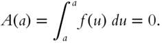
Let ![]() be any antiderivative of
be any antiderivative of ![]() . Then the area function is equal to
. Then the area function is equal to
where ![]() is an arbitrary constant. Set
is an arbitrary constant. Set ![]() . Then
. Then

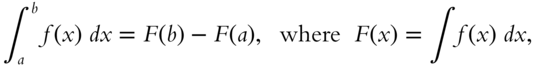
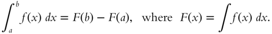
Therefore ![]() . Hence the area under the curve
. Hence the area under the curve ![]() is equal to
is equal to
Now set ![]() . Then the definite integral
. Then the definite integral ![]() corresponds to the area under the curve of the function
corresponds to the area under the curve of the function ![]() for
for ![]() . This can be determined by calculating the value of any antiderivative
. This can be determined by calculating the value of any antiderivative ![]() of
of ![]() at
at ![]() and subtracting the value of
and subtracting the value of ![]() at
at ![]() .
.
The definite integral is commonly written as

Go to 349.
349
Fundamental Theorem of Calculus:
The significance of the result in the last frame is that determining the area does not require calculating the limit of the summation in the definition of the definite integral (which can be a difficult calculation) but merely evaluating any antiderivative at the endpoints of the interval.
In frame 336, we discussed the convention for determining the sign for the area. Note that a definite interval can be positive or negative for some interval. If a function ![]() is negative in some interval, then the definite integral evaluated in that interval will be negative.
is negative in some interval, then the definite integral evaluated in that interval will be negative.
Summary: We have shown that for any continuous function ![]() ,
,
where ![]() .
.
This relation is so extraordinary that it is called the fundamental theorem of calculus.
Go to 350.
350
To see how all this works, we will find the area under the curve ![]() between
between ![]() and
and ![]() .
.
In this example an antiderivative is ![]() because
because ![]() . Therefore
. Therefore

Note that the definite integral yields a number. Furthermore, we no longer need to introduce an undetermined constant ![]() whenever we evaluate an expression such as
whenever we evaluate an expression such as ![]() .
.
Go to 351.
351
Can you find the area under the curve ![]() , between the points
, between the points ![]() and
and ![]() ?
?
If right, go to 353.
Otherwise, go to 352.
352
The solution is straightforward. An antiderivative for the function ![]() is
is ![]() . Therefore
. Therefore
Go to 353.
353
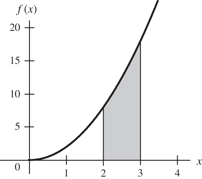
Find the area under the curve ![]() between
between ![]() and
and ![]() .
.
Go to 354.
354
An antiderivative for the function ![]() is
is ![]() . Therefore
. Therefore
Let's introduce a little labor‐saving notation. Frequently we have to find the difference of an expression evaluated at two points, as ![]() . This is often denoted by
. This is often denoted by
For example, ![]() . Using this notation, the solution to this problem is written
. Using this notation, the solution to this problem is written
Note that this area is negative.
Go to 355.
355
Here is another practice problem:
The graph shows a plot of ![]() . Find the area between the curve and the
. Find the area between the curve and the ![]() ‐axis from
‐axis from ![]() and
and ![]() .
.
- Answer: [5 | ¼ | 4 |
 |
|  | none of these]
If right, go to 357.
Otherwise, go to 356.
356
Here is how to do the problem: one antiderivative is ![]() . You can check that
. You can check that ![]() . Therefore
. Therefore

Go to 357.
357
To help remember the definition of definite integral, try writing it yourself. Write an expression defining the definite integral of ![]() between the limits
between the limits ![]() and
and ![]() .
.
To check your answer, go to 358.
358
The answer is
Congratulations if you wrote this or an equivalent expression. If you wrote
your statement is true, but it is not the definition of a definite integral. The result is true because both sides represent the same thing—the area under the curve of ![]() between
between ![]() and
and ![]() . It is an important result because without it the definite integral would be much more difficult to calculate; however, it is not true by definition.
. It is an important result because without it the definite integral would be much more difficult to calculate; however, it is not true by definition.
The definite integral appears merely to provide a second way to find the area under a curve. To compute the area, we were led back to the indefinite integral, but we could have found the area directly from the indefinite integral. The importance of the definite integral arises from its definition as the limit of a sum. The process of dividing a system into small elements and then adding them together is a powerful technique that is applicable to more problems than finding the area under a curve. These invariably lead to definite integrals, which we can evaluate in terms of indefinite integrals by using the fundamental theorem of calculus (frame 349).
Go on to 359.
359
Can you prove that

After you have tried to prove this result, go to 360.
360
The proof that ![]() is as follows:
is as follows:
Reversing the limits of the integral yield,
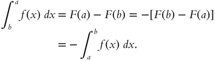
Go to 361.
361
Which of the following expressions correctly gives ![]() ?
?
Go to 362.
362
The answer is

It is easy to see why this result is true by inspecting the figure.

The integral yields the total area under the curve, from 0 to ![]() , which is the sum of the area
, which is the sum of the area ![]() between 0 to
between 0 to ![]() , and
, and ![]() between
between ![]() and
and ![]() . But
. But ![]() is negative, because
is negative, because ![]() is negative in that region. By symmetry, the two areas just add to 0. However, you should be able to find
is negative in that region. By symmetry, the two areas just add to 0. However, you should be able to find ![]() or
or ![]() separately. Try this problem:
separately. Try this problem:

If right, go to 364.
Otherwise, go to 363.
363
The answer is
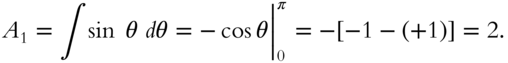
If you forgot the integral, you can find it in frame 312. In evaluating ![]() at the limits,
at the limits, ![]() , and
, and ![]() .
.
Go to 364.
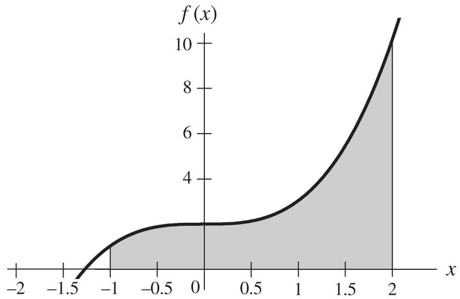
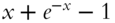
364
Here is a graph of the function ![]() .
.
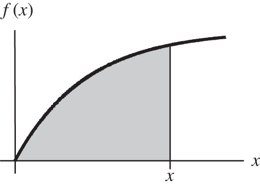
Can you find the shaded area under the curve between the origin and ![]() ?
?
- Answer: [e−x | 1 − e−x | x + e−x | x + e−x − 1]
Go to 366 if you did this correctly.
See 365 for the solution.
365
Here is the solution to 364.
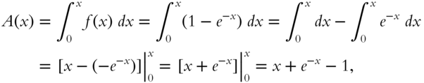
The area is bounded by a vertical line through ![]() . Our result gives
. Our result gives ![]() as a variable that depends on
as a variable that depends on ![]() . If we choose a specific value for
. If we choose a specific value for ![]() , we can substitute it into the above formula for
, we can substitute it into the above formula for ![]() and obtain a specific value for
and obtain a specific value for ![]() . We have obtained a definite integral in which one of the boundary points is left as a variable.
. We have obtained a definite integral in which one of the boundary points is left as a variable.
Go to 366.
366
Let's evaluate one more definite integral before going on. Find:

(If you need to, use the integral tables, frame 312.)
- Answer: [0 | 1 | ∞ | π | π/2 | none of these]
If you got the right answer, go to 368.
If you got the wrong answer, or no answer at all, go to 367.
367
From the integral table, frame 312, we see that
Therefore,
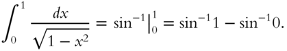
Because ![]() , we have that
, we have that ![]() . Similarly, sin−1 0 = 0. Thus, the integral has the value
. Similarly, sin−1 0 = 0. Thus, the integral has the value ![]() .
.
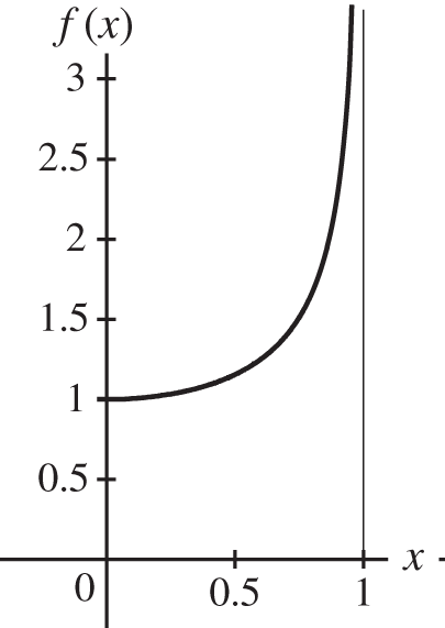
A graph of ![]() is shown above. Although the function is discontinuous at x = 1, the area under the curve is perfectly well defined.
is shown above. Although the function is discontinuous at x = 1, the area under the curve is perfectly well defined.
Go to 368.
3.4 Some Applications of Integration
368
In this section we are going to apply integral calculus to a few problems.
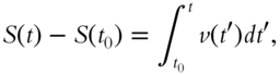
In Chapter 2 we learned how to find the velocity of a particle if we know its position in terms of time. Now we can reverse the procedure and find the position from the velocity. For instance, we are in an automobile driving along a straight road through thick fog. To make matters worse, our mileage indicator is broken. Instead of watching the road all the time, let's keep an eye on the speedometer. We have a good watch along, and we make a continuous record of the speed starting from the time when we were at rest. The problem is to find how far we have gone. More specifically, given ![]() , how do we find the change in position of the automobile
, how do we find the change in position of the automobile ![]() , called the displacement, when we were at rest? Because the automobile is traveling in the same direction, the change of position is equal to the distance traveled.
, called the displacement, when we were at rest? Because the automobile is traveling in the same direction, the change of position is equal to the distance traveled.
Try to work out a method.
To check your result, go to 369.
369
Because ![]() , we must have
, we must have ![]() (as was shown in frame 275). Now let us integrate both sides from the initial point
(as was shown in frame 275). Now let us integrate both sides from the initial point ![]() to the final point in order to find the change in position of the automobile
to the final point in order to find the change in position of the automobile

where we have replaced the integration variable by ![]() .
.
If you did not get this result, or would like to see more explanation, go to 370.
Otherwise, go to 371.
370
Another way to understand this problem is to look at it graphically. Here is a plot of ![]() as a function of
as a function of ![]() .
.
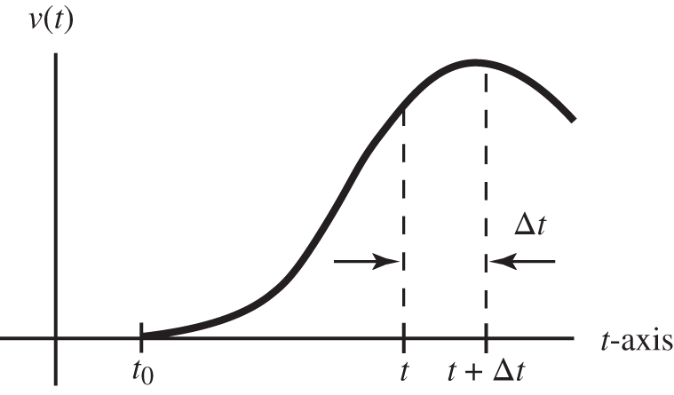
In time ![]() the distance traveled is
the distance traveled is ![]() . The total distance traveled is thus equal to the area under the curve between the initial time and the time of interest, and this is
. The total distance traveled is thus equal to the area under the curve between the initial time and the time of interest, and this is ![]() . There may be some confusion because the same symbol
. There may be some confusion because the same symbol ![]() , which is the dependent variable of the function, appears both as an endpoint of the integral and as the integration variable in the integrand
, which is the dependent variable of the function, appears both as an endpoint of the integral and as the integration variable in the integrand ![]() . The integration variable is what we call a dummy variable and we can denote it by any symbol, for example,
. The integration variable is what we call a dummy variable and we can denote it by any symbol, for example, ![]() . Thus the integral is written as
. Thus the integral is written as
Often this distinction between the dependent variable of the function and the integration variable is not explicit but implicit, and the symbol ![]() is used in both places, as we will do in a few frames.
is used in both places, as we will do in a few frames.
Go to 371.
371
Suppose an object moves with a velocity that continually decreases in the following way, ![]() (
( ![]() and
and ![]() are positive constants).
are positive constants).

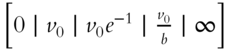
At ![]() the object is at the origin;
the object is at the origin; ![]() . Which of the following is the distance,
. Which of the following is the distance, ![]() , the object will have moved after an infinite time (or, if you prefer, after a very long time)?
, the object will have moved after an infinite time (or, if you prefer, after a very long time)?
- Answer:
If correct, go to 373.
Otherwise, go to 372.
372
Here is the solution to the problem of frame 371.
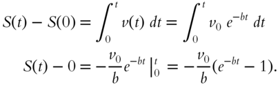
We are interested in the ![]() . Because e−bt → 0 as t → ∞, we have
. Because e−bt → 0 as t → ∞, we have

Although the object never comes completely to rest, its velocity gets so small that the total distance traveled is finite.
Go to 373.
373
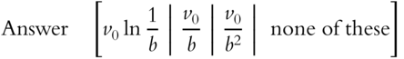
Not all integrals give finite results. For example, try this problem.
A particle starts from the origin at ![]() with a velocity
with a velocity ![]() , where
, where ![]() and
and ![]() are constants. How far does it travel as
are constants. How far does it travel as ![]() ?
?
Go to 374.
374
It is easy to see that problem 373 leads to an infinite integral.

(The last step uses formula 6, frame 312.)
Because ![]() as
as ![]() , we see that
, we see that ![]() as
as ![]() . In this case, the particle is always moving fast enough so that its motion is unlimited. Or, alternatively, the area under the curve
. In this case, the particle is always moving fast enough so that its motion is unlimited. Or, alternatively, the area under the curve ![]() increases without limit as
increases without limit as ![]() .
.
Go to 375.
375
The Method of Slices:
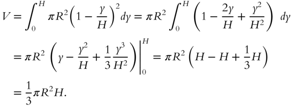
Integration can be used for many tasks besides calculating the area under a curve. For example, it can be used to find the volumes of solids of known geometry. A general method for this is explained in frame 395. However, one can calculate the volume of symmetric solids by a simple extension of methods we have learned already. In the next few frames we are going to find the volume of a right circular cone.
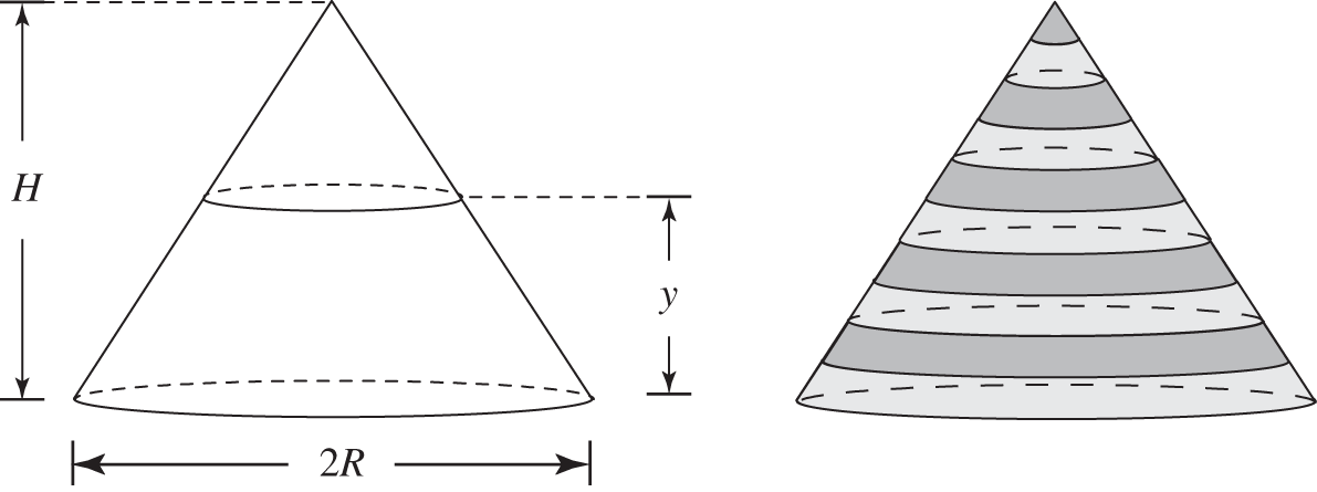
The height of the cone is ![]() , and the radius of the base is
, and the radius of the base is ![]() . We will let
. We will let ![]() represent distance vertically from the base.
represent distance vertically from the base.
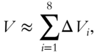
Our method of attack, called the method of slices, is similar to that used in frame 378 to find the area under a curve. We will slice the body into a number of discs whose volume is approximately that of the cone in the figure (the cone has been approximated by ten circular discs). Then we have
where ![]() is the volume of one of the discs. In the limit where the height of each disc (and hence the volume) goes to 0, we have
is the volume of one of the discs. In the limit where the height of each disc (and hence the volume) goes to 0, we have

In order to evaluate this, we need an expression for ![]() .
.
Go to frame 376.
376
Because we are going to take the limit where ![]() , we will represent the volume element by
, we will represent the volume element by ![]() from the start.
from the start.
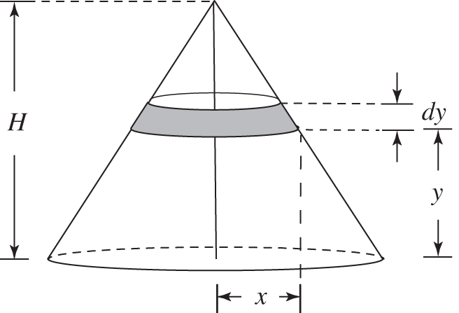
A section of the cone is shown in the figure, which for our purposes is represented by a disc. The radius of the disc is ![]() and its height is
and its height is ![]() . Try to find an expression for
. Try to find an expression for ![]() in terms of
in terms of ![]() . (You will have to find
. (You will have to find ![]() in terms of
in terms of ![]() .)
.)
To check your result, or to see how to obtain it, go to 377.
377
The answer is:
If you got this answer, go on to 378. If you want to see how to derive it, read on.
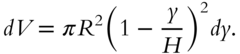
The volume of this disc is the product of the area and height. Thus, ![]() . Our remaining task is to express
. Our remaining task is to express ![]() in terms of
in terms of ![]() . The diagram shows a cross-section of the cone.
. The diagram shows a cross-section of the cone.

Because ![]() and
and ![]() are corresponding edges of similar triangles, it should be clear that
are corresponding edges of similar triangles, it should be clear that

Thus,

Go to 378.
378
We now have an integral for V.

Try to evaluate this.
To check your answer, go to 379.
379
The result is ![]() Congratulations, if you obtained the correct answer. Go on to 380.
Congratulations, if you obtained the correct answer. Go on to 380.
Otherwise, read below:
Go to 380.
380
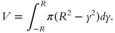
Let's find the volume of a sphere. Can you write an integral that will give the volume of the hemisphere?

(The slice of the hemisphere shown in the drawing may help you in this.)
Go to 381 to check your formula.
381
The answer is
If you wrote this, go ahead to frame 382. Otherwise, read on.
In order to calculate the volume of the sphere, consider a disk of thickness ![]() and radius
and radius ![]() , located at a distance
, located at a distance ![]() from the center of the sphere as shown in the drawing in frame 280. The differential volume
from the center of the sphere as shown in the drawing in frame 280. The differential volume ![]() of the disk between
of the disk between ![]() and
and ![]() is
is ![]() . By the Pythagorean theorem
. By the Pythagorean theorem ![]() , therefore
, therefore ![]() .
.
As you add up the disks, the limits of the variable ![]() are
are ![]() to
to ![]() . The volume integral is
. The volume integral is

Go to 382.
382
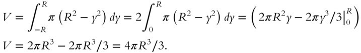
Now go ahead and evaluate the integral

To see the correct answer, go to 383.
383
The answer is
Go to 384.
384
Here's a problem that involves finding the area under a curve and the volume of a solid of revolution generated by the curve.

What is the area under the curve ![]() , for the range
, for the range ![]() to
to ![]() ?
?
![]()
Go to 385.
385
Here is how to solve the problem. The area under the curve is the integral
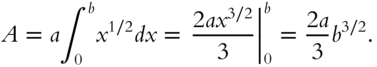
Go to 386.
386
Now rotate that area about the ![]() ‐axis to generate the volume shown in the diagram.
‐axis to generate the volume shown in the diagram.
Can you use the method of slices to write an integral that will give the volume? (The slice in the drawing may help you visualize this.)
Go to 387 to check your formula.
387
The answer is ![]() . If you wrote this, go ahead to frame 388. Otherwise, read on.
. If you wrote this, go ahead to frame 388. Otherwise, read on.
Consider a disk of thickness ![]() and radius
and radius ![]() , located at a distance
, located at a distance ![]() from the origin as shown in the diagram. The differential volume
from the origin as shown in the diagram. The differential volume ![]() for the disk is
for the disk is
The limits of the variable ![]() are
are ![]() to
to ![]() . Now you can set up the volume integral
. Now you can set up the volume integral
Go to 388.
388
Now go ahead and evaluate the integral.
To see the answer, go to 389.
389
The answer is

Go to 390.
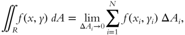
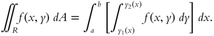
3.5 Multiple Integrals
390
The subject of this section—multiple integrals—introduces some new concepts and enables us to apply calculus to a world of problems that involve multiple variable calculus, in contrast to single variable calculus.
The integrals we have discussed so far, of the form ![]() , have had a single independent variable, usually called
, have had a single independent variable, usually called ![]() . Double integrals are similarly defined for two independent variables,
. Double integrals are similarly defined for two independent variables, ![]() and
and ![]() . In general, multiple integrals are defined for an arbitrary number of independent variables, but we will only consider two. Note that up to now
. In general, multiple integrals are defined for an arbitrary number of independent variables, but we will only consider two. Note that up to now ![]() has often been the dependent variable:
has often been the dependent variable: ![]() . In this section, however,
. In this section, however, ![]() along with
along with ![]() will always be independent variables, and
will always be independent variables, and ![]() will be the dependent variable. Thus,
will be the dependent variable. Thus, ![]() is a function of two variables.
is a function of two variables.
In frame 349 the definite integral of ![]() between
between ![]() and
and ![]() was defined by
was defined by

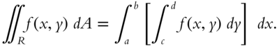
The double integral is similarly defined, but with two independent variables. There are, however, some important differences. For a single definite integral the integration takes place over a closed interval between ![]() and
and ![]() on the
on the ![]() ‐axis. In contrast, the integration of
‐axis. In contrast, the integration of ![]() takes place over a closed region
takes place over a closed region ![]() in the
in the ![]() plane.
plane.
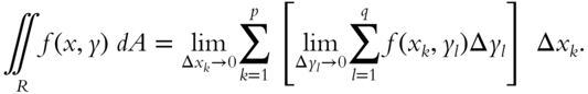
To define the double integral, divide the region ![]() into
into ![]() smaller regions each of area
smaller regions each of area ![]() .
.

Let ![]() be an arbitrary point inside the region
be an arbitrary point inside the region ![]() . Then in analogy to the integral of a single variable, the double integral is defined as
. Then in analogy to the integral of a single variable, the double integral is defined as

Go to 391.
391
The double integral is often evaluated by taking ![]() to be a small rectangle with sides parallel to the
to be a small rectangle with sides parallel to the ![]() and
and ![]() axes. The procedure is first evaluate the sum and limit along one direction and then along the other. Consider the upper portion of the region
axes. The procedure is first evaluate the sum and limit along one direction and then along the other. Consider the upper portion of the region ![]() in the
in the ![]() plane to be bounded by the curve
plane to be bounded by the curve ![]() , while the lower portion is bounded by
, while the lower portion is bounded by ![]() , as in the diagram.
, as in the diagram.
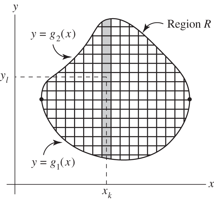
If we let ![]() , then
, then

This is a complicated expression, but it can be simplified by carrying it out in two separate steps. Let us insert some brackets to clarify the separate steps.
The first step is to carry out the operation within the brackets. Note that ![]() is not altered as we sum over
is not altered as we sum over ![]() in the brackets. This corresponds to summing over the crosshatched strip in the diagram with
in the brackets. This corresponds to summing over the crosshatched strip in the diagram with ![]() treated as approximately a constant. The quantity in square brackets is then merely a definite integral of the variable
treated as approximately a constant. The quantity in square brackets is then merely a definite integral of the variable ![]() , with
, with ![]() treated as a constant. Note that although the limits of integration,
treated as a constant. Note that although the limits of integration, ![]() and
and ![]() , are constants for a particular value of
, are constants for a particular value of ![]() , they are in general non‐constant functions of
, they are in general non‐constant functions of ![]() . The quantity in square brackets can then be written as
. The quantity in square brackets can then be written as
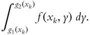
This quantity will no longer depend on ![]() , but it will depend on
, but it will depend on ![]() both through the integrand
both through the integrand ![]() and the limits
and the limits ![]() ,
, ![]() . Consequently,
. Consequently,

In calculations it is essential that one first evaluate the integral in the square brackets while treating ![]() as a constant. The result is some function, which depends only on
as a constant. The result is some function, which depends only on ![]() . The next step is to calculate the integral of this function with respect to
. The next step is to calculate the integral of this function with respect to ![]() , treating
, treating ![]() now as a variable.
now as a variable.
Go to 392.
392
Multiple integrals are most easily evaluated if the region ![]() is a rectangle whose sides are parallel to the
is a rectangle whose sides are parallel to the ![]() and
and ![]() coordinate axes, as shown in the drawing.
coordinate axes, as shown in the drawing.
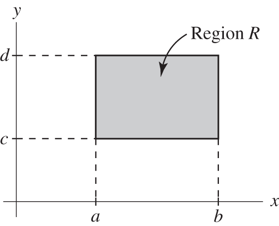
The double integral is
As an exercise to test your understanding, how would the above expression be written if the integration over ![]() were to be carried over before the integration over
were to be carried over before the integration over ![]() ?
?
Go to 393.
393
When ![]() is chosen to be integrated first, the double integral becomes
is chosen to be integrated first, the double integral becomes

This can be found merely by interchanging the ![]() and
and ![]() operations in evaluating the double integral. (Note that the integration limits must also be interchanged.)
operations in evaluating the double integral. (Note that the integration limits must also be interchanged.)
To see how this works, let us evaluate the double integral of ![]() over the rectangle in the
over the rectangle in the ![]() plane bounded by the lines
plane bounded by the lines ![]() ,
, ![]() ,
, ![]() , and
, and ![]() . The double integral is equal to the iterated integral.
. The double integral is equal to the iterated integral.

Alternatively we could have written
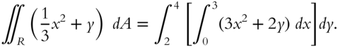
Evaluate each of the above expressions. The answers should be the same.
If you made an error or want more explanation, go to 394.
Otherwise, go to 395.
394
Integrating first over ![]() and then over
and then over ![]() yields
yields
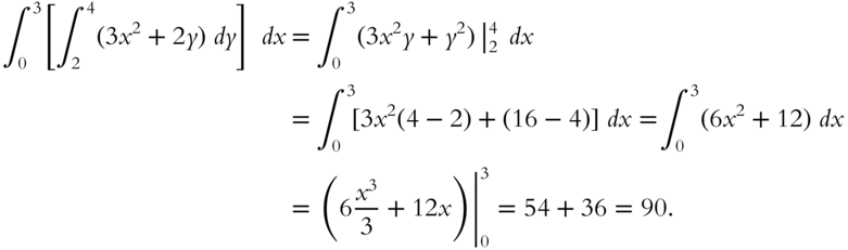
Integrating first over ![]() and then over
and then over ![]() yields
yields
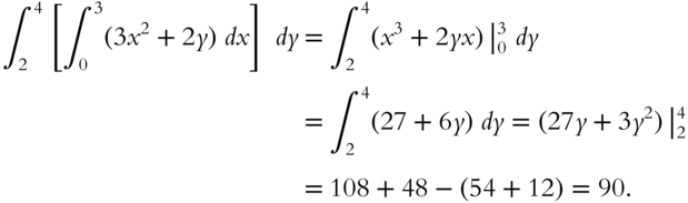
Go to 395.
395
Just as the equation ![]() defines a curve in the two‐dimensional
defines a curve in the two‐dimensional ![]() plane, the equation
plane, the equation ![]() defines a surface in the three‐dimensional space because that equation determines the value of
defines a surface in the three‐dimensional space because that equation determines the value of ![]() for any values assigned independently to
for any values assigned independently to ![]() and
and ![]() .
.

We can easily see from the above definition of the double integral that ![]() is equal to the volume
is equal to the volume ![]() of space under the surface
of space under the surface ![]() and above the region
and above the region ![]() . In this case
. In this case ![]() is the height of column above
is the height of column above ![]() . Therefore,
. Therefore, ![]() is approximately equal to the volume of that column. The sum of all these columns is then approximately equal to the volume under the surface. In the limit as
is approximately equal to the volume of that column. The sum of all these columns is then approximately equal to the volume under the surface. In the limit as ![]() , the sum defining the double integral becomes equal to the volume under the surface and above
, the sum defining the double integral becomes equal to the volume under the surface and above ![]() , so
, so
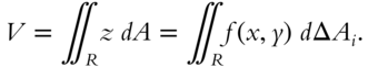
Calculate the volume under the surface defined by ![]() and above the rectangle whose sides are determined by the lines
and above the rectangle whose sides are determined by the lines ![]() ,
, ![]() ,
, ![]() , and
, and ![]() .
.
![]()
Go to 396.
396
The answer is 36. If you obtained this result, go to frame 397. If not, study the following.
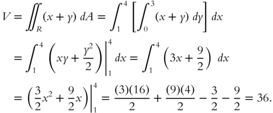
The iterated integral could just as well have been evaluated in the opposite order.
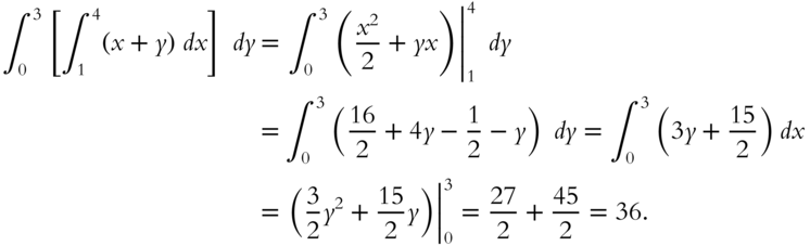
Go to 397.
397

The bottom of this plow‐shaped solid is in the form of an isosceles triangle with base ![]() and height
and height ![]() . When oriented along the
. When oriented along the ![]() axes as shown, its thickness is given by
axes as shown, its thickness is given by ![]() , where
, where ![]() is a constant. The problem is to find an expression for the volume.
is a constant. The problem is to find an expression for the volume.
To check your answer, go to 398.
398
The volume is ![]() . Read on if you want an explanation; otherwise go to 399.
. Read on if you want an explanation; otherwise go to 399.

The base of the object forms a triangle, as shown. The integral can be carried out with respect to ![]() and
and ![]() in either order. We shall integrate first over
in either order. We shall integrate first over ![]() .
.

From the drawing, 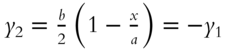 , so that
 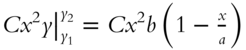 , and
, and
The integral can also be evaluated in reverse order. The calculation is simplified by making use of symmetry; the volume is twice the volume over the upper triangle. Thus

where  . The answer is the same,
 ![]() .
.
Go to 399.
Conclusion to Chapter 3
399
Well, here you are at the last frame of Chapter 3. At this point you should understand the principles of integration and be able to do some integrals. With practice your repertoire will increase. Don't be afraid to use integral tables—everyone does. You can find them online, for instance, https://en.wikipedia.org/wiki/Lists_of_integrals.
Summary of Chapter 3
3.1 Antiderivative, Integration, and the Indefinite Integral (frames 306–314)
When a function ![]() is differentiated to give
is differentiated to give ![]() , then
, then ![]() is an antiderivative of
is an antiderivative of ![]() , that is,
, that is, ![]() If
If ![]() is an antiderivative of
is an antiderivative of ![]() , then all the antiderivatives of
, then all the antiderivatives of ![]() can be denoted by writing
can be denoted by writing

where ![]() is arbitrary constant. The expression
is arbitrary constant. The expression ![]() is also called the integral of
is also called the integral of ![]() . The symbol
. The symbol ![]() is known as the integration symbol, and represents the inverse of differentiation. It is important not to omit this constant. Otherwise the answer is incomplete.
is known as the integration symbol, and represents the inverse of differentiation. It is important not to omit this constant. Otherwise the answer is incomplete.
Indefinite integrals are often found by hunting for an expression that when differentiated gives the integrand ![]() . Thus from the earlier result that
. Thus from the earlier result that
we have that
By starting with known derivatives as in Table 1, a useful list of integrals can be found. Such a list is given in frame 312 and for convenience is repeated in Table 2. You can reconstruct the most important of these formulas from the differentiation expressions in Table 1. More complicated integrals can often be found in large integral tables.
3.2 Some Techniques of Integration (frames 315–334)
Often an unfamiliar function can be converted into a familiar function having a known integral by using a technique called change of variable which is related to the chain rule of differentiation and uses the relation
Another valuable technique is integration by parts, as described by the relation proved in frame 324.
Frequently a number of different integration procedures are used in a single problem as illustrated in frames 329–331.
The method of partial fractions (frame 332) involves splitting a function into a sum of fractions with simpler denominators that can be integrated by other methods.
3.3 Area under a Curve and Definite Integrals (frames 335–367)
The area ![]() under the curve of a function
under the curve of a function ![]() between
between ![]() and
and ![]() can be found by dividing the area into N narrow strips parallel to the y‐axis, each of area
can be found by dividing the area into N narrow strips parallel to the y‐axis, each of area ![]() , and summing the strips. In the limit as the width of each strip approaches zero, the limit of the sum approaches the area under the curve.
, and summing the strips. In the limit as the width of each strip approaches zero, the limit of the sum approaches the area under the curve.
This infinite sum is called a definite integral and is denoted by
The area function ![]() has the variable
has the variable ![]() for the upper limit of the definite integral in frame 341, and the integration variable is renamed
for the upper limit of the definite integral in frame 341, and the integration variable is renamed ![]() .
.
The area function ![]() is an antiderivative of the function
is an antiderivative of the function ![]() (frame 346),
(frame 346), ![]() . Therefore, it is an indefinite integral.
. Therefore, it is an indefinite integral.

where ![]() is any particular antiderivative of
is any particular antiderivative of ![]() , and
, and ![]() is an arbitrary constant. If we want to know the area bounded by
is an arbitrary constant. If we want to know the area bounded by ![]() and some value
and some value ![]() , the constant
, the constant ![]() can be evaluated by noting that if
can be evaluated by noting that if ![]() , then the area is zero, so
, then the area is zero, so ![]() and
and ![]() . Therefore,
. Therefore, ![]() The area under the curve between
The area under the curve between ![]() and
and ![]() is then
is then
This result is called the fundamental theorem of integral calculus (frame 349). The significance of the result in the last frame is that determining the area does not require calculating the limit of the summation in the definition of the definite integral but merely evaluating any antiderivative at the endpoints of the interval.
3.4 Some Applications of Integration (frames 368–389)
If we know v(t), the velocity of a particle as a function of t, we can obtain the position of the particle as a function of time by integration. We saw earlier that ![]() , so
, so ![]() , and if we integrate both sides of the equation from the initial point
, and if we integrate both sides of the equation from the initial point ![]() to the final point
to the final point ![]() , we have the change of position of the particle, called the displacement,
, we have the change of position of the particle, called the displacement,
where we have replaced the integration variable by ![]() .
.
Applications of integration in finding volumes of symmetric solids are given in frames 375–389.
3.5 Multiple Integrals (frames 390–399)
Multiple integrals may be defined for an arbitrary number of independent variables. We discuss two variables because the procedures for an arbitrary number are merely generalizations of those that apply to two independent variables. The double integral over a region ![]() in the
in the ![]() plane of the function
plane of the function ![]() is defined as
is defined as
as discussed in frames 390–391. The double integral can be evaluated by integrating over one variable while holding the other variable constant, in either order.
Continue to Chapter 4.
Notes
- Answers: Frame 306: antiderivative, or
- Frame 308: − cos x + c
- Answer: Frame 325:
- Answers: Frame 351:

- Frame 353: −15
- Answer: Frame 355:

- Answers: Frame 361: 0
- Frame 362: 2
- Frame 364:
- Answer: Frame 366:

- Answer: Frame 371:

- Answer: Frame 373: none of these
- Answer: Frame 393: 90