![]()
Importing and Creating Data
When you are loading data into R, you have a number of options. For external files, there are several functions that read specific kinds of files or data. R also comes with a number of data sets that can be loaded. Sometimes the user wants to create data. R has a multitude of random number generators for data creation. Data can be entered manually using c() or by using various other functions to create data with certain patterns.
The first section of this chapter covers reading data into R and loading R data sets. The second section covers probability distributions, including random number generators and the function sample(). The third section covers manual data entry and creating data with patterns.
Reading Data into R, Including R Data Sets
There are a number of R functions that read data into R. The most common ones are scan() to read data of a given mode, and read.table() and read.csv() to read data from a matrix structured table. Some of the more exotic ones are read.fortran() to read data coded in FORTRAN format, read.fwf() for reading tables in fixed width format, read.xls() for Excel spreadsheets (the creators of R recommend against reading a Excel file directly but provide some functions to do so), and read.delim() for tab delineated columns. For a complete listing, see http://cran.r-project.org/doc/manuals/r-release/R-data.html.
The Function scan()
The function scan() imports data from a file row-by-row, either from the values to the argument text or directly from the console. For importing a file, the rows do not have to be of the same length. The function reads data of the modes logical, numeric, complex, character, raw, and list. For all of the modes except list, all of the data must be readable as the mode.
The function scan() is most often used to read an external file. The reference to the file comes first in the call and must be contained within quotes. The reference may be relative to the location of the workspace or an absolute location—including URLs. An example is
> scan("test.txt")
Read 7 items
[1] 1 3 5 7 1 4 6
where test.txt is a file containing the seven digits in two rows. To browse for a file, enter file.choose() for the quoted file reference, that is scan(file.choose()).
The function can also be used to read in data at the console, which is done by setting the data equal to an argument called text, where the data is in quotation marks. For example:
> scan(text = "1 2 3 4")
Read 4 items
[1] 1 2 3 4
Data can also be read in directly from the console by setting the file equal to “ ”. For example:
> scan("")
1: 1
2: 4
3: 9
4: 3
5:
Read 4 items
[1] 1 4 9 3
Here R cues for a data point with the point number followed by a colon. To stop entering data, use control-z in Windows and control-d in Linux, or enter a blank line by pressing the return(enter) key.
If the mode of the data being entered is not numeric, the argument what must be included in the call to scan(). The argument what is set equal to mode(), where mode is the mode of the data. For example:
> scan("test.txt", what=complex())
Read 7 items
[1] 1+0i 3+0i 5+0i 7+0i 1+0i 4+0i 6+0i
which reads complex data from the external file test.txt. If the data in the file is not readable as the mode, scan() returns an error.
The function scan() also has the argument sep, which tells scan() the separator between values in either an external file or in the value of text. By default, the separator is white space. The argument sep can be set to any one-byte value that R can read. In the call to scan(), the value for sep is placed within quotation marks. For example:
> scan(text = "1, 2, 3, 4", sep=",")
Read 4 items
[1] 1 2 3 4
Here a comma is used as the separator between data values.
If two separating symbols in the call to scan() do not have a value between the two, then by default the value is set to NA. For example:
> scan(text = "1, 2, 3,, 4", sep=",")
Read 5 items
[1]  1  2  3 NA  4
For data with header lines, the argument skip tells scan() to skip lines before reading data. The value of skip tells scan() how many lines to skip and can be of any atomic mode. The value is coerced to an integer if possible or else interpreted as zero. If skip equals zero, no lines are skipped.
To read a header line, the argument nlines tells scan() to read lines up to and including the value of nlines. Like skip, nlines can be of any atomic mode and scan() coerces the value to integer. If nlines is set to zero, all lines are read.
The function scan() returns a vector. To create a matrix or array, the call to scan() can be part of a call to matrix() or array(). For example:
> matrix(scan( text="1 2 3 4 5 6 7 8 9 10" ), 2, 5, byrow=T)
Read 10 items
     [,1] [,2] [,3] [,4] [,5]
[1,]    1    2    3    4    5
[2,]    6    7    8    9   10
There are several other arguments for scan() that do things such as limit the number of data points to be read, fill out lines of incomplete data, or tell scan() the style of the decimal point in the data. More information can be found by entering ?scan at the R prompt.
The Functions read.table(), read.csv(), and read.delim()
The three functions read.table(), read.csv(), and read.delim() are essentially the same function, differing only in the default values of the argument sep and the argument header. As with the function scan(), the argument sep gives the symbol used to separate values of the data in the file and can be any one byte value. The argument header takes on logical values and tells the function whether to read a header from the first line or not.
The three functions import data from a file, where the file is in the form of a matrix, or from values of the argument text. If the data is from a file, the location of the file is entered first in the call within quotation marks. The location of the file can be relative to the workspace or absolute, including URLs. To browse for a file, enter file.choose() for the quoted name, for example, read.table(file.choose()). An example with a quoted name follows:
> read.table("test2.txt")
   V1 V2 V3 V4
1 one  3  5  7
2 two  4  6  8
Note that the columns do not have to be of the same mode. Here the file test2.txt contains both character and numeric data and is in the same folder as the R workspace.
If the rows in the file are not all of the same length, by default the function will return an error. The argument fill is a logical argument and tells R to fill out rows that have fewer elements than other rows. For example:
> read.table("test4.txt", fill=T)
   V1 V2 V3 V4
1 one  3  5  7
2 two  4  6 NA
Here test4.txt is missing the last element of the second row. R fills in the element with NA.
If the argument text is used to enter a table, the end of a row is indicated by . For example:
> read.table(text="1 2 3 4
 2 3 4 5")
  V1 V2 V3 V4
1  1  2  3  4
2  2  3  4  5
For read.table(), the default value for sep is white space and the default value for header is FALSE. For read.csv(), the default value for sep is a comma and the default value for header is TRUE. For read.delim(), the default value for sep is a tab—which in R is entered as —and the default value for header is TRUE. (There are two other related functions, read.csv2() and read.delim2(), which are for European use and have dec, the style of the decimal point, set equal to ‘ , ’, and, for read.csv2(), sep set equal to ;.)
The three functions create a data.frame out of the data, so the modes of the elements only need to be consistent down the columns. If a column contains character data, then by default the column is converted to a factor. By setting the argument as.is to TRUE, the conversion is to character. For example:
> read.table("test3.txt", sep=",")
   V1    V2 V3 V4
1 one     1  3  4
2   1  four  3  2

> class(read.table("test3.txt", sep=",")[,1])
[1] "factor"

> class(read.table("test3.txt", sep=",")[,3])
[1] "integer"

> read.table("test3.txt", sep=",", as.is=T)
   V1    V2 V3 V4
1 one     1  3  4
2   1  four  3  2

> class(read.table("test.txt3", sep=",", as.is=T)[,1])
[1] "character"

> class(read.table("test.txt3", sep=",", as.is=T)[,3])
[1] "integer"
You can see the difference between not setting as.is and setting as.is to TRUE. The file test3.txt is a file in the same folder as the workspace, is in matrix form, and contains both character and integer data.
The three functions can read some types of atomic data: logical, numeric, complex, and character. From the R help page for the three functions, R reads in the data as character data and then converts from character to one of the classes logical, integer, numeric, complex, or factor.
As noted above, if as.is is set to TRUE, columns containing character data are not converted to factors but retain the class character. The argument as.is can also be entered as a logical vector with a value for each column. A shorter vector can be entered also, with the values cycling across the columns.
The argument colClasses manually sets the class of each column and can be used in place of as.is to keep a column in character mode. The possible values for the column classes are NA, NULL, logical, integer, numeric, complex, raw, character, factor, Date or POSIXct. The values are quoted, except for NA and NULL, and are entered as a vector. The values will cycle.
If the value is NA, the normal conversion will take place. Otherwise, if possible, the column elements are coerced to the class listed for the column. For example:
> read.table("test2.txt", colClasses=c("character","factor",NA,NA))
   V1 V2 V3 V4
1 one  3  5  7
2 two  4  6  8

> class(read.table("test2.txt", colClasses=c("character","factor",NA,NA))[,1])
[1] "character"

> class(read.table("test2.txt", colClasses=c("character","factor",NA,NA))[,2])
[1] "factor"

> class(read.table("test2.txt", colClasses=c("character","factor",NA,NA))[,3])
[1] "integer"
The arguments row.names and col.names are used to give names to the rows and columns of the data.frame. For row.names, the argument can be a character vector of length equal to the number of rows in the data.frame; the argument can be an integer specifying which column in the data.frame to use as row names; or the argument can be a character value containing the name of the column to be used as the row names. The row names do not cycle.
For col.names, the argument is a character vector of names for the columns. The vector must be of the same length as the number of columns. If col.names is not specified and header is FALSE, then the columns are named V1, V2,…, Vn, where n is the number of the last column.
If header is TRUE and the first column does not have a name, while the rest of the columns do, then R sets the first column as the row names.
Some examples are the following:
For the matrix
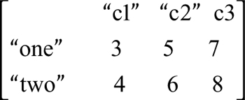
which is the file test5.txt, the example is
> read.table("test5.txt", header=T)
    c1 c2 c3
one  3  5  7
two  4  6  8
Note that header is TRUE, and there is one less row in the first column.
For a matrix consisting of the second two rows of test5.txt, called test6.txt, an example follows:
> read.table("test6.txt", col.names=c("c1","c2","c3","c4"), row.names=2)
   c1 c3 c4
3 one  5  7
4 two  6  8
The four names are assigned to the four columns and then column two is used for the names of the rows while the other columns retain the assigned names.
There are several other arguments for the functions read.table(), read.csv(), and read.delim(). A full description of the functions can be found by entering ?read.table at the R prompt.
R comes with a number of data sets. Some of these data sets are found in the package datasets, which is one of the packages installed by default in R. To load data sets from the package datasets, enter library(datasets) at the R prompt. To see the data sets in datasets, enter library(help=datasets) at the R prompt. Once the library is loaded, the data sets in datasets are accessible by entering the name of the data set.
For any library, once the library is loaded, the data sets in the library are accessible like any other object in the workspace. The packaged data sets are not necessarily data.frames, but many are.
Other Functions to Import Files
Other functions for importing files will not be covered here. A search on read, done by entering ??read at the R prompt, gives many of the functions that read into the R workspace.
For Excel spreadsheets, the R writers recommend exporting an Excel spreadsheet to a .csv (comma separated values) file and reading the .csv file into R. There are a few functions to read Excel spreadsheets, but the R writers say the conversion is full of pitfalls.
Probability Distributions and the Function sample()
R has a wealth of random number generators. The random number generators are one of four functions associated with the probability distributions, all of which are covered here. The functions associated with probability distributions mostly have the same form. Many of the distributions can be found by entering ??distributions at the R prompt. Entering ?distribution at the R prompt gives the distributions—and generators—in the package stats.
Probability Distributions
For the probability distributions in the package stats, there are four functions associated with a distribution: ddist(), pdist(), qdist(), and rdist(), where dist describes the distribution. For example, for the normal distribution, dist equals norm. Not all distributions have all four.
The first function is the function for the density. The function, ddist(), gives the heights of the probability density function at specified values of a vector of numbers. The second function is for the cumulative probability. The function, pdist(), by default gives the areas under the probability density function to the left of the specified values of a vector of numbers.
The third function is for quantiles. The function, qdist(), by default gives the values on the real line for which the areas to the left of the values are equal to the values of a specified vector of probabilities. The fourth function is the random number generator. The function, rdist(), generates pseudorandom variables from the distribution. For all of the functions, the vectors can be vectors of length one.
The four functions have arguments to specify the standard parameters of the given distribution, for many of which there are defaults. For example, for the normal distribution the arguments are mean and sd and are set equal to 0 and 1 by default. Both the variables mean and sd can be entered as vectors and will cycle. The vectors must be numeric or logical. Logical vectors are coerced to numeric. The distributions in the package stats are given in Table 9-1 along with the parameter arguments for the distributions.
Table 9-1. Probability Distributions in Package Stats
Distribution Name in R |
Parameters of the Distribution |
|---|---|
beta |
shape1=1, shape2=2, npc=0 |
binom |
size, prob |
birthday |
classes=365, coincident=2 |
cauchy |
location=0, scale=1 |
chisq |
df, npc=0 |
exp |
rate=1 |
f |
df1, df2, npc |
gamma |
shape, rate=1, scale=1/rate |
geom |
prob |
hyper |
m, n, k |
lnorm |
meanlog=0, sdlog=1 |
multinom |
size, prob |
nbinom |
size, prob, mu |
norm |
mean=0, sd=1 |
pois |
lambda |
signrank |
n |
t |
df, ncp |
tukey |
nmeans, df, nranges=1 |
unif |
min=0, max=1 |
weibull |
shape, scale=1 |
wilcox |
m, n |
The prefixes are d, p, q, r. The multinom function only has d and r. The tukey function only has p and q. The birthday function only has p and q and does not have a log.p argument. From the CRAN help page for distribution.
For all of the four functions, the first argument is required and does not have a default. For the density functions, the first argument x is a vector of real numbers or values that can be coerced to real numbers. For the cumulative probability functions, the first argument q is also a vector of real numbers or values that can be coerced to real numbers. For the quantile functions, the first argument p is a vector of probabilities or values that can be coerced to a value between zero and one inclusive. For the random number generators, the first argument n (nn for the hypergeometric, sign rank, and wilcox distributions) is a positive integer, or a value that can be coerced to integer, that tells R how many numbers to generate.
In general, for the density functions, if the values of the first argument are to be considered as logs of the values of interest, the logical argument log is set to TRUE. For the probability and quantile functions, the logical argument log.p is set to true if the values that are for the probabilities are entered or output as logs of the probabilities.
In general, for the cumulative probability and quantile functions, whether to use the upper tail or the lower tail of the distribution can be set using the logical argument lower.tail. The lower tail is set by default. Lower tails are the area under the distribution function for values less than or equal to the values of the first argument, and upper tails are the area under the distribution function for values greater than the values of the first argument.
Also, in general, parameters can be entered as vectors and will cycle. If an illegal value for a parameter is entered, the function will give an error.
More information about a given probability distribution can be found by entering ?ddist at the R prompt, where dist is the name of the distribution from Table 9-1, except for the tukey and birthday distributions for which ?pdist works.
The Function sample()
Sometimes a random sample is needed rather than random numbers. The function sample() takes a random sample of atomic objects, list objects, or any other mode object for which length is defined.
The function sample() takes four arguments. The first argument, x, is the object to be sampled. If x is a single positive real number greater than one, sample() samples from the sequence from 1 to the real number rounded down to an integer. If x is an object that can be coerced to a vector or a single positive number and no other arguments are given, sample() returns a permutation of the object or the sequence from one to the number rounded down to an integer.
The second argument size is the number of items to be sampled. The argument size can be a nonnegative integer or a real number that can be rounded down to a nonnegative integer.
The third argument is the logical argument replace, which tells sample() whether to sample with replacement. The default value is FALSE, that is to sample without replacement. If size is larger than the length of x and replace is FALSE, then sample() will give an error.
The fourth argument is prob and gives a list of weights for the sampling. The argument prob must be of the same length as x, must have elements that can be coerced to non-negative numeric elements and for which at least half of the coerced elements are nonzero. The coerced elements of prob do not have to sum to one.
For example:
> sample(10)
 [1]  8 10  6  4  7  5  3  9  1  2

> sample(10, 5)
[1] 3 1 6 8 9

> sample(c("a1", "a2", "a3"), 6, replace=T)
[1] "a1" "a1" "a1" "a3" "a3" "a1"

> sample(11:21, prob=1:11)
 [1] 18 20 14 21 19 17 12 16 15 13 11
More information about sample() can be found by entering ?sample at the R prompt.
Manually Entering Data and Generating Data with Patterns
Data can be entered manually using the function c(), where the c stands for collect. Sometimes data with a certain pattern is needed, for example, in setting up indices for matrix or array manipulation or as input to functions. There are a number of functions in R that give patterned results, which can be useful. Sometimes indexed names are needed for dimensions in a vector, matrix, or array. The function paste() can be used to create indexed names.
The Function c()
The function c() collects objects together into a single object. The objects to be collected are separated by commas within the call to c(). The objects can be NULL, raw, logical, integer, double, character strings (which must be quoted), named objects (which must be atomic objects, lists, or expressions), lists, and/or expressions. Objects can also be functional calls that return any of the above classes.
If all of the objects in the call are atomic objects, the function c() collects the objects into a vector of the elements making up the objects. The class of the resulting vector is the highest level class within the elements of the vector, where the levels of the classes increase in the order NULL, raw, logical, integer, double, complex, and character.
An example of the hierarchy follows:
> rw = as.raw(c(36, 37, 38, 39))

> rw
[1] 24 25 26 27

> c(rw, rw)
[1] 24 25 26 27 24 25 26 27

> c(rw, TRUE)
[1] TRUE TRUE TRUE TRUE TRUE

> c(rw, 40)
[1] 36 37 38 39 40

> c(rw, 40.5)
[1] 36.0 37.0 38.0 39.0 40.5

> c(rw, 1+1i)
[1] 36+0i 37+0i 38+0i 39+0i  1+1i

> c(rw, "six")
[1] "24"  "25"  "26"  "27"  "six"
The conversion from raw is automatic except for the conversion to character, which maintains the raw values.
The function c() has one possible named argument, the logical argument recursive. The default value of recursive is FALSE. If recursive is set to TRUE and the collection contains a list but not an expression, then the list is taken apart to the lowest level of the individual elements in the list and a vector of atomic elements is returned. The object takes on the class of the highest level of class in the object. If recursive is FALSE, the resulting object becomes a list.
In the hierarchy of classes, list is above the atomic classes but below expression. If an expression is included in the call to c(), then the result has class expression.
An example for objects of class list and expression follows:
> a.list
[[1]]
     cl1 cl2
[1,]   1   3
[2,]   2   4

[[2]]
[1] "abc" "cde"

> c(a.list, 1:2)
[[1]]
     cl1 cl2
[1,]   1   3
[2,]   2   4

[[2]]
[1] "abc" "cde"

[[3]]
[1] 1

[[4]]
[1] 2

> c(a.list, 1:2, recursive=T)
[1] "1"   "2"   "3"   "4"   "abc" "cde" "1"   "2"

> a.expr = expression(y ~ x, `1`)

> c(a.list, a.expr)
expression(1:4, c("abc", "cde"), y ~ x, `1`)
In the first call to c(), an object of class list is returned. In the second call, an object of class character is returned. In the third call, an object of class expression is returned.
Names can be assigned to the elements of the object created by c() by setting the elements equal to a name in the listing—for example:
> c(a=1,b=2,3)
a b
1 2 3
Here the first two elements are assigned the names a and b while the third element is not assigned a name.
More information about c() can be found by entering ?c at the R prompt.
The Functions seq() and rep()
The functions seq() and rep() are used for sequences and repeated patterns. In the simplest form, using seq() is the same as using the colon operator to create a sequence. However, seq() can create more sophisticated sequences than the colon operator. The function rep() repeats the first argument to the function a specified number of times, where there are two possible ways to do the repetition.
The function seq() has six arguments. The first two arguments are the starting and ending values of the sequence and are named from and to. The arguments from and to can take on logical, numeric, or complex values. For logical values, TRUE is coerced to one and FALSE is coerced to zero. For complex values, the imaginary part is dropped. Both to and from are set to one by default.
The third argument is by. The argument by gives the value by which to increment the sequence. The argument can also take on logical, numeric, and complex values; however, it cannot equal FALSE since FALSE coerces to zero and by cannot equal zero. The argument does not have to divide into the difference between to and from evenly. The sequence will stop at the largest value less than or equal to to if to is greater than from. If to is less than from, then by must be negative and the sequence stops at the smallest value greater than or equal to to.
The fourth argument is length.out. By default, length.out is set to NULL. The argument length.out can be used in place of by. The argument gives the length of the sequence to be output. If length.out is specified, by defaults to (to - from) / (length.out-1).
The fifth argument is along.with. The argument along.with is also used in place of by. The length of the sequence to be output is given by the length of along.with. The sixth argument is the argument … for any arguments to or from lower-level functions used by seq(). Some examples follow:
> seq(3)
[1] 1 2 3
Entering just one value without a name gives a sequence from one to the largest integer less than or equal to the value for positive values or the smallest integer greater than or equal to the value if the value is negative.
> seq(3, 10)
[1]  3  4  5  6  7  8  9 10
When two values are entered without names, the first is interpreted as the from value, the second is interpreted as the to value, and by is set equal to one.
> seq(3, 10, 2)
[1] 3 5 7 9
When three values are entered without names, the first is interpreted as the from value, the second is interpreted as the to value, and the third is interpreted as the by value.
> seq(3, 10, len=4)
[1]  3.000000  5.333333  7.666667 10.000000
Here, length.out is shortened to len.
 > seq(3, 10, along=c(1,2,1,2))
[1]  3.000000  5.333333  7.666667 10.000000
Here, along.with is shortened to along.
> seq(c(1,2,1,2))
[1] 1 2 3 4
If a vector with more than one element is entered as the only argument, a sequence starting with one is created, with by equal to one, and of length equal to the length of the vector.
> seq(len=4)
[1] 1 2 3 4

> seq(7,along=c(1,2,1,2))
[1]  7  8  9 10

> seq(7,len=4)
[1]  7  8  9 10
Entering length.out or along.with alone or with a value for from returns a vector staring with the value of from, with by equal to 1, and of the correct length. For long sequences, there are lower level functions that are faster. See the help page for seq(). More information about seq() can be found by entering ?seq at the R prompt.
The function rep() repeats the first argument in a pattern determined by the other the arguments. The first argument can be any type of object that can be coerced to a vector. The other three arguments are times, each, and length.out. The default values for times, each, and length.out in the S3 system are 1, 1, and NA, respectively.
The argument times is a vector of values that can be coerced to integer. The argument must be either a single value or of the same length as the first argument. If the argument takes a single value, the first argument is repeated the number of times of the single value.
If the argument times is of length equal to the length of the first argument, then each element of the first argument is repeated the number of times indicated by the corresponding element of the argument times. The argument times is the second argument to rep(). For example:
> rep(0,5)
[1] 0 0 0 0 0

> rep(1:3, 5)
 [1] 1 2 3 1 2 3 1 2 3 1 2 3 1 2 3

> rep(1:3, 2:4)
[1] 1 1 2 2 2 3 3 3 3
Here, the second argument is not explicitly called times, but times implicitly takes on the value.
The argument each can be any object that can be coerced to a vector of integers, where the first element is non-negative. Only the first element of the object is used. The argument tells rep() to repeat each element of the first argument each times. For example:
> rep(1:3, each=3)
[1] 1 1 1 2 2 2 3 3 3
>
> rep(1:3, each=3, times=2)
 [1] 1 1 1 2 2 2 3 3 3 1 1 1 2 2 2 3 3 3
>
> rep( rep(1:3, times=2:4), each=2)
 [1] 1 1 1 1 2 2 2 2 2 2 3 3 3 3 3 3 3 3
>
> rep( rep(1:3, times=2:4), times=2)
 [1] 1 1 2 2 2 3 3 3 3 1 1 2 2 2 3 3 3 3
The last argument is length.out. The argument can take on any value that can be coerced to an integer vector and for which the first element is non-negative. Only the first element is used. If length.out is set to a value, only the number of elements given by the value of the argument is returned. For example:
> rep( rep(1:3, times=2:4), times=2, len=8)
[1] 1 1 2 2 2 3 3 3
Here, length.out is shortened to len.
More information about rep() can be found by entering ?rep at the R prompt.
Combinatorics and Grid Expansion
Combinatorics is a subject about the combinations that can be made from a set of discrete values. Combinations are all of the combinations that are possible from a discrete set of values for a given number of elements in each combination, where no element is repeated. Permutations are the set of all possible permutations of a given size from a discrete set of elements. Grid expansion is about the expansion of different sets of elements so that each element of each set is linked with every element of the other sets. Probably the easiest way to see what the combinations, permutations, and grid expansion involve is by showing some examples.
Three functions that are relevant are combn(), permsn()—which is in library prob—and expand.grid. The function combn() takes the arguments x, m, FUN, simplify, and … . The argument x is any object that can be coerced to a vector and is the discrete set from which the combinations are formed. The argument m is the number of elements to include in each combination. The argument FUN is an optional function to operate on the elements of x. The argument simplify is logical. If TRUE, an array or matrix is returned. If FALSE, a list is returned. The default value is TRUE. The argument … contains any arguments for FUN. For example:
> combn(1:3,2)
     [,1] [,2] [,3]
[1,]    1    1    2
[2,]    2    3    3
Note that the combinations are down the rows.
The function permsn() is in the package prob. Since the package is not one of the packages installed by default, the package may need to be installed. (See Chapter 1.) If the package is installed, the package must be loaded with
library(prob)
The function permsn() takes just two arguments, x and m, which are as described for combn(). Following is an example for permsn():
> permsn(1:3,2)
     [,1] [,2] [,3] [,4] [,5] [,6]
[1,]    1    2    1    3    2    3
[2,]    2    1    3    1    3    2
Note that the permutations are down the rows. Also note that while combn() just has the combination (1,2), permsn() includes both (1,2) and (2,1) and so forth. The function permsn() returns a matrix.
The function expand.grid() takes objects as arguments. The objects are separated by commas and must be able to be coerced to a vector. The function returns the vectors crossed with each other in a data frame. For example:
> expand.grid(1:2,3:4,5:6)
  Var1 Var2 Var3
1    1    3    5
2    2    3    5
3    1    4    5
4    2    4    5
5    1    3    6
6    2    3    6
7    1    4    6
8    2    4    6
Here, the combinations are across the rows.
More information about combn(), permsn(), and expand.grid() can be found by entering ?combn, ?prob::permsn, and ?expand.grid at the R prompt. Note that if prob is not installed, the second command will not work.
The Function Paste
This chapter ends with the function paste(). The function is used to create character strings out of any type of object. Other than the objects to be strung together, which are separated by commas, paste takes two arguments, sep and collapse. The argument sep gives the value of what is to separate the individual terms and is by default a white space. The argument sep must be a character string or character object. To set the value to nothing, set sep equal to “”.
The argument collapse is also a character string or object and is used to separate results.
One of the useful applications of paste()is the creation of dimension names. Here is an example of three simple applications of paste(). The second example would be appropriate for creating dimension labels.
> paste("a", 1:3)
[1] "a 1" "a 2" "a 3"
>
> paste("a", 1:3, sep="")
[1] "a1" "a2" "a3"
>
> paste("a", 1:3, sep="", collapse="+")
[1] "a1+a2+a3"
You can find more information about paste() by entering ?paste at the R prompt.