This book would not be complete without advice on some tricky parts of R. When it seems that everything is set up right, but things still do not do what you expect and you do not know why, this chapter can help. This chapter also describes some not-so-obvious parts of R.

Value Substitution: NA, NaN, Inf, and -Inf

This section has to do with missing data (NA) or illegal elements (NaN, Inf, or -Inf). Say you want to substitute a value, for example 0, for missing values. The intuitive approach would be to enter something like the following:

mat[ mat==NA ] = 0

This does not work. What does work is to enter the following:

mat [ is.na(mat) ] = 0

For example:

> mat = matrix(c(1,NA,3,4),2,2)
> mat
     [,1] [,2]
[1,]    1    3
[2,]   NA    4
  
> mat[ mat==NA ]=2
> mat
     [,1] [,2]
[1,]    1    3
[2,]   NA    4
  
> mat[ is.na(mat) ]=2
> mat
     [,1] [,2]
[1,]    1    3
[2,]    2    4

The same method works for illegal values. The values NaN, Inf, and -Inf are defined in R for illegal operations. For example:

> 1/0
[1] Inf
  
> -1/0
[1] -Inf
 
> 0/0
[1] NaN
  
> log(-1)
[1] NaN
Warning message:
In log(-1) : NaNs produced

In this example, dividing a positive number by zero results in plus infinity; dividing a negative number by zero gives negative infinity; dividing zero by zero is not defined, so NaN is returned. Trying to find the logarithm of minus one returns NaN with a warning since the logarithm of minus one is not defined.

The functions is.finite(), is.infinite(), and is.nan() take the place of is.na() in tests for finite, Inf and -Inf, and NaN elements. For example:

> mat = matrix(c(1,NaN,Inf,-Inf),2,2)
> mat
     [,1] [,2]
[1,]    1  Inf
[2,]  NaN -Inf
 
> mat[is.finite(mat)]=2
> mat
     [,1] [,2]
[1,]    2  Inf
[2,]  NaN -Inf
  
> mat[is.infinite(mat)]=3
> mat
     [,1] [,2]
[1,]    2    3
[2,]  NaN    3
  
> mat[is.nan(mat)]=4
> mat
     [,1] [,2]
[1,]    2    3
[2,]    4    3

Note that is.infinite() treats Inf and -Inf the same.

The function sign() returns -1 for an argument equal to -Inf. As a result, a simple way to handle the sign problem is to take the sign of the object first, and then multiply the absolute value of the object resulting from the substitution by the sign object after assigning a number to -Inf. For example:

> mat=matrix(c(1,2,Inf,-Inf),2,2)
> mat
     [,1] [,2]
[1,]    1  Inf
[2,]    2 -Inf
  
> sg.mat = sign(mat)
> sg.mat
     [,1] [,2]
[1,]    1    1
[2,]    1   -1
  
> mat[is.infinite(mat)] = 4
> mat
     [,1] [,2]
[1,]    1    4
[2,]    2    4
  
> mat = sg.mat*abs(mat)
> mat
     [,1] [,2]
[1,]    1    4
[2,]    2   -4

You can find more information about NA and is.na() by entering ?is.na at the R prompt. You can find more information about NaN, Inf, -Inf, is.nan(), is.finite(), and is.infinite()by entering ?is.finite at the R prompt.

If Statements and Logical Vectors

Often when a logical test is done, the objects being tested are of length greater than one. R does not like this and gives a warning that only the first logical element is used. Suppose you want to test whether any element of a logical object is TRUE. Then the function any() is useful. The function any() returns TRUE if there are any TRUEs in the object, and FALSE otherwise. For example:

> a.logical=c(T,T,F,T)
> a.logical
[1]  TRUE  TRUE FALSE  TRUE
> test=8
> test
[1] 8
  
> if (a.logical==T) test=1
Warning message:
In if (a.logical == T) test = 1 :
  the condition has length > 1 and only the first element will be used
> test
[1] 1
  
> if (any(a.logical)) test=2
> test
[1] 2
 
> if (any(!a.logical)) test=3
> test
[1] 3
  
> if (any(!a.logical[1:2])) test=4
> test
[1] 3

Note that in the third and fourth tests, the test is for FALSEs. The ! is used to logically negate the object as.logical in the test for FALSEs.

You can find more information about any()by entering ?any at the R prompt.

Lists and the Functions list() and c()

Adding to lists can be confusing. Do you use list() or c()? When creating a list, the elements to be entered into the list are separated by commas. But say you want to add some elements. Then you will usually want to use c(). For example:

> a.list = list(1:4, paste("a",1:7,sep=""))
> a.list
[[1]]
[1] 1 2 3 4
 
[[2]]
[1] "a1" "a2" "a3" "a4" "a5" "a6" "a7"
 
> b.list = list(a.list,1:3)
> b.list
[[1]]
[[1]][[1]]
[1] 1 2 3 4
 
[[1]][[2]]
[1] "a1" "a2" "a3" "a4" "a5" "a6" "a7"
 
[[2]]
[1] 1 2 3
 
> c.list = c(a.list,1:3)
> c.list
[[1]]
[1] 1 2 3 4
 
[[2]]
[1] "a1" "a2" "a3" "a4" "a5" "a6" "a7"
 
[[3]]
[1] 1
 
[[4]]
[1] 2
 
[[5]]
[1] 3
 
> d.list = c(a.list,list(1:3))
> d.list
[[1]]
[1] 1 2 3 4
 
[[2]]
[1] "a1" "a2" "a3" "a4" "a5" "a6" "a7"
 
[[3]]
[1] 1 2 3

The object d.list is probably what you wanted as a result. (Another method to get the same results is to use append() instead of c() in the above expressions.)

Getting Data out of Functions

When you are writing functions, sometimes the purpose of the function is to print results to the console; sometimes the purpose is to export an object—which will be written to the console if not assigned to an object; and sometimes both types of output are needed. The functions print() and cat() write to the console. To output an object, the object must be the last statement in the function. For example:

> a.function = function() {
  print(1:3)
  print(5:6)
  }
 
> a.function()
[1] 1 2 3
[1] 5 6
 
> a.result = a.function()
[1] 1 2 3
[1] 5 6
 
> a.result
[1] 5 6

Since the two sequences are in print functions in the example, the sequences are printed out whether an assignment takes place or not. Note that only the second sequence is assigned to the object a.result, since the print statement for the second sequence is the last statement in the function before the close bracket. For another example, the print() function is removed:

> a.function = function() {
  1:3
  5:6
  }
 
> a.function()
[1] 5 6
 
> a.result = a.function()
 
> a.result
[1] 5 6

In this example, since there is no print() function, the sequences are not printed. The second sequence, being the last statement, is returned by the function.

Recursive Functions

R functions can be applied recursively. A recursive function is a function that calls itself until a condition is met. We use the series that defines the exponential distribution to illustrate the workings of a recursive function.

Recall that.

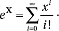
So, we want a function that adds at each step for i equal to 0, 1, …, n for some stopping point n. Since decreases at each step and gets arbitrarily small, we used the size of to set the stopping point.

The function follows:

> r.exp =
function(x,i=0) {
 if (abs( x^i/factorial(i) ) > 1.0e-8) {
 
  r.exp(x,i+1) + x^i/factorial(i)
 
 }
 else {
  0
 }
}

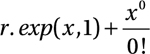
At the first step of the recursion, i equals zero, so the value of r.exp() is

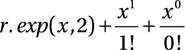
At the second step, the value is

If i equal to n is the last step before is less than our stopping point of 1.0e-8, then for i equal to n, the value of r.exp() equals

But

so the recursion stops. Since the expression in the if section of the function is the last statement executed in the function, the function returns the result.

To see how the function works, we let x equal one:

> r.exp(1)
[1] 2.718282
 
> exp(1)
[1] 2.718282

Note that for x equal to one, the function gives the same value as the function exp().

Some Final Comments

R is a great program. In this last section, we give some final comments.

First, there is a class that we should have included earlier, the class formula. Formulas such as y~x are of class formula and can be assigned a name. Formulas are used in many of the modeling functions or as a way of grouping the object on the left by the values of the objects on the right, for example in boxplot(). In boxplot(), a box plot is created for the values on the left of the tilde for each combination of the values on the right of the tilde.

On the left of the tilde is one object that can be a vector or a matrix and that is the dependent variable(s). On the right of the tilde are the independent variables separated by plus or minus signs. See the help page for formula for information about crossing and nesting variables as well as not including various variables—such as the intercept term or a specific interaction. You can open the help page by entering ?formula at the R prompt.

R takes some determination to use. If you get stuck on a problem and cannot find an answer, do not be afraid to experiment. You cannot break R. If you are creating functions, remember to try to figure out a way to use indices rather than loops. Take the process in small steps. And remember that data frames are lists, not matrices.