7
SEARCHING FOR ANSWERS

For all the problems we have encountered so far, there was a direct method to compute the solution. But this is not always the case. For many problems, we have to search for the solution using some type of algorithm, such as when solving a Sudoku puzzle or the n-queens problem. In these cases, the process involves trying a series of steps until either we find the solution or we have to back up to a previous step to try an alternative route. In this chapter we’ll explore a number of algorithms that allow us to efficiently select a path that leads to a solution. Such an approach is known as a heuristic. In general, a heuristic isn’t guaranteed to find a solution, but the algorithms we explore here (thankfully) are.
Graph Theory
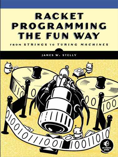
It’s often the case that a problem we’re trying to solve can be modeled with a graph. Intuitively, a graph is just a set of points (or nodes) and connecting lines, as illustrated in Figure 7-1. Each node represents some state of the problem-solving process, and the lines extending from one node to other nodes represent possible alternative steps. We’ll first give some basic graph definitions as background before delving into the actual problem-solving algorithms.
The Basics
Formally, a graph is a finite set V of vertices (or nodes) and a set E of edges joining different pairs of distinct vertices (see Figure 7-1).

Figure 7-1: Graph
In Figure 7-1 above, V = {a, b, c, d, e} are the vertices and E = {(a, b), (a, c), (b, c), (c, d), (b, e), (e, d)} are the edges.
A sequence of graph vertices (v1, v2, …, vn), such that there’s an edge connecting vi and vi+1, is called a walk. If all the vertices are distinct, a walk is called a path. A walk where all the vertices are distinct except that v1 = vn is called a cycle or circuit. In Figure 7-1, the sequence (a, b, c, b) is a walk, the sequence (a, b, c, d) is a path, and the sequence (a, b, c, a) is a cycle.
A graph with a path from each vertex to every other vertex is said to be connected. A connected graph without any cycles is called a tree. In a tree, any path is assumed to flow from upper nodes to lower nodes. Such a structure (where there are no cycles and there is only one way to get from one node to another) is known as a directed acyclic graph (DAG). It’s possible to convert the graph above to a tree by removing some of its edges, as shown in Figure 7-2.
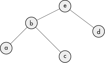
Figure 7-2: Tree
If nodes x and y are connected in such a way that it’s possible to go from x to y, then y is said to be a child node of x. Nodes without child nodes (such as a, c, and d) are known as terminal (or leaf) nodes. Problems that have solutions modeled by a tree structure lend themselves to simpler search strategies since a tree doesn’t have circuits. Searching a graph with circuits requires keeping track of nodes already visited so that the same nodes aren’t re-explored.
It’s possible to label each edge of the graph with a numerical value called a weight, as shown in Figure 7-3. This type of graph is called a weighted graph.
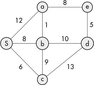
Figure 7-3: Weighted graph
If e is an edge, the weight of the edge is designated by w(e). Weights can be used to represent any number of measurements such as time, cost, or distance, which may affect the choice of edge when searching a graph.
A number of interesting questions arise when exploring the properties of graphs. One such question is this: “Given any two nodes, what’s the shortest path between them?” Another is the famous traveling salesman problem: “Given a list of cities and the distances between them, what’s the shortest possible route that visits each city exactly once and returns to the original city?” This last question, where each node is visited exactly once and returns to the original node, involves what is called a Hamiltonian circuit.
Graph Search
There are two broad categories of strategies for searching graphs: breadth-first search (BFS) and depth-first search (DFS). To illustrate these concepts, we’ll use the tree in Figure 7-2.
Breadth-First Search
Breadth-first search involves searching a graph by fully exploring each level (or depth) before moving on to the next level. In the tree diagram (shown in Figure 7-2), the e (root) node is on the first level, nodes b and d are on the next level, and nodes a and c are on the third level. This typically involves using a queue to stage the nodes to be examined. The process begins by pushing the root node onto the queue, as shown in Figure 7-4:
Figure 7-4: A queue containing the root node
We then pop the first node in the queue (e) and test it to see if it’s a goal node; if not, we push its child nodes onto the queue, as shown in Figure 7-5:
Figure 7-5: The queue after node e was explored
Again we pop the first node in the queue (this time b) and test it to see if it’s a goal node; if not, we push its child nodes onto the queue, as shown in Figure 7-6:

Figure 7-6: The queue after node b was explored
We continue in this fashion until a goal node has been found, or the queue is empty, in which case there’s no solution.
Depth-First Search
Depth-first search works by continuing to walk down a branch of the tree until a goal node is found or a terminal node is reached. For example, starting at the root node of the tree, nodes e, b, and a would be examined in order. If none of those node are goal nodes, we back up to node b and examine its next child node, c. If c is also not a goal node, we back all the way up to e and examine its next child node, d. The n-queens problem in the next section provides a simple example of using depth-first search.
The N-Queens Problem
The n-queens problem is a classic problem often used to illustrate depth-first search. The problem goes like this: position n queens on an n-by-n chess-board such that no queen is attacked by any other queen. In case you aren’t familiar with chess, a queen can attack any square on the same row, column, or diagonal that the queen lies on, as illustrated in Figure 7-7.

Figure 7-7: A queen’s possible moves
The smallest value of n for which a solution exists is 4. The two possible solutions are shown in Figure 7-8.
Figure 7-8: Solutions to the 4-queens problem
One reason for the popularity of this problem is that the search graph is a tree, meaning that with a depth-first search, there’s no possibility that a state previously seen will be reached again (that is, once a queen is placed, it’s not possible to get to a state with fewer queens in subsequent steps). This avoids the annoying need to keep track of previous states to ensure they aren’t explored again.
A simple approach to this problem is to go column by column, testing each square in a column and continuing until a solution has been reached (backtracking as required). For example, if we begin with Figure 7-9, we can’t place a queen at b1 or b2, because it would be attacked by the queen at a1.
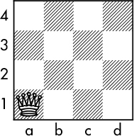
Figure 7-9: First queen at a1
The next available square that’s not attacked is b3, resulting in Figure 7-10:

Figure 7-10: Second queen at b3
But now when we get to column c, we’re stuck since every square in that column is attacked by one of the other queens. So we backtrack and move the queen in column b to b4 in Figure 7-11:
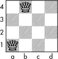
Figure 7-11: Second queen at b4
So now we can place a queen on c2 in Figure 7-12:
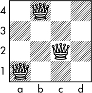
Figure 7-12: Third queen at c2
Alas, now there’s no spot for a queen on column d. So we backtrack all the way to column a and start over in Figure 7-13.

Figure 7-13: Backtrack to first queen at a2
The process continues in this manner until a solution is found.
A Racket Solution
We define the chessboard as an n-by-n array constructed from a mutable vector with n elements, each of which is also an n-element vector, where each element is either a 1 or a 0 (0 means the square is unoccupied; 1 means the square has a queen):
(define (make-chessboard n)
  (let loop ([v n] [l '()])
    (if (zero? v)
        (list->vector l)
        (loop (sub1 v) (cons (make-vector n 0) l)))))
To allow accessing elements of the chessboard cb by a row (r) and column (c) number, we define the following accessor forms, where v is the value being set or retrieved.
(define (cb-set! cb r c v)
  (vector-set! (vector-ref cb c) r v))

(define (cb-ref cb r c)
  (vector-ref (vector-ref cb c) r))
Since we’re using a mutable data structure for the chessboard, we’ll need a mechanism to copy the board whenever a solution is found, to preserve the state of the board.
(define (cb-copy cb)
  (for/vector ([v cb]) (vector-copy v)))
We’ll of course need to be able to see the solutions, so we provide a print procedure:
(define (cb-print cb)
  (let ([n (vector-length cb)])
    (for* ([r n]
           [c n])
      (when (zero? c) (newline))
      (let ([v (cb-ref cb r c)])
        (if (zero? v)
            (display " .")
            (display " Q")
            ))))
  (newline))
The actual code to solve the problem, dfs, is a straightforward depth-first search. As solutions are found, they’re compiled into a list called sols, which is the return value of the function. In the code below, recall that in the let loop form, we’re employing a named let (which we described in Chapter 3) where we’re defining a function (loop) that we’ll call recursively.
(define (dfs n)
  (let ([sols '()]
        [cb (make-chessboard n)])
    (let loop([r 0][c 0])
      (when (< c n)
     ➊ (let ([valid (not (attacked cb r c))])
          (when valid
         ➋ (cb-set! cb r c 1)
         ➌ (if (= c (sub1 n))
              (let ([copy (cb-copy cb)])
             ➍ (set! sols (cons copy sols)))
           ➎ (loop 0 (add1 c)))
         ➏ (cb-set! cb r c 0))
       ➐ (when (< (add1 r) n) (loop (add1 r) c)))))
 ➑ sols))
The code first tests each position to see whether the current cell is being attacked by any of the queens that have already been placed on the board ➊ (the code for attacked will be described shortly); if not, then that cell is marked as valid, and a queen (the number 1) is placed on that square ➋. Next we test whether the current square is in the final column of the board ➌; if it is, we’ve found a solution, so a copy of the board is placed in sols ➍. If we’re not on the last column, we then nest down to the next level (that is, the next column) ➎. Finally, the valid square is cleared ➏ so that additional rows in the column can be tested ➐. Once all the solutions have been found, they’re returned ➑.
Where the DFS backtracking occurs in this process is a bit subtle. Suppose we’re at a position that is under attack by the previously placed queens, so valid ➊ is false and execution falls through ➐. Now suppose we’re also on the last row. In that case, the test fails ➐, so no further looping occurs and the recursive call returns. Either there are no following statements, in which case the entire loops exits, or there there additional statements to execute after returning from the recursive call. This can only occur where the current position is cleared and we’re at a previous location ➏. This is the backtrack point. Execution then resumes at the last when statement ➐.
The following function tests whether a square is under attack by any of the previously placed queens. It only checks the columns prior to the current column since the other columns of the chessboard haven’t yet been populated.
(define (attacked cb r c)
  (let ([n (vector-length cb)])
    (let loop ([ac (sub1 c)])
      (if (< ac 0) #f
          (let ([r1 (+ r (- c ac))]
                [r2 (+ r (- ac c))])
            (if (or (= 1 (cb-ref cb r ac))
                    (and (< r1 n) (= 1 (cb-ref cb r1 ac)))
                    (and (>= r2 0) (= 1 (cb-ref cb r2 ac))))
                #t
                (loop (sub1 ac))))))))
To output the solutions, we define a simple routine to iterate through and print each solution returned by dfs.
(define (solve n)
  (for ([cb (dfs n)]) (cb-print cb)))
Here are a couple of test runs.
> (solve 4)

 . Q . .
 . . . Q
 Q . . .
 . . Q .
 . . Q .
 Q . . .
 . . . Q
 . Q . .

> (solve 5)

 . . Q . .   . . . Q .  . . . . Q   . Q . . .   . . . . Q
 . . . . Q   . Q . . .  . Q . . .   . . . . Q   . . Q . .
 . Q . . .   . . . . Q  . . . Q .   . . Q . .   Q . . . .
 . . . Q .   . . Q . .  Q . . . .   Q . . . .   . . . Q .
 Q . . . .   Q . . . .  . . Q . .   . . . Q .   . Q . . .

 . Q . . .   . . . Q .   . . Q . .   Q . . . .  Q . . . .
 . . . Q .   Q . . . .   Q . . . .   . . Q . .  . . . Q .
 Q . . . .   . . Q . .   . . . Q .   . . . . Q  . Q . . .
 . . Q . .   . . . . Q   . Q . . .   . Q . . .  . . . . Q
 . . . . Q   . Q . . .   . . . . Q   . . . Q .  . . Q . .

> (solve 8)

 . . Q . . . . .
 . . . . . Q . .
 . . . Q . . . .
 . Q . . . . . .
 . . . . . . . Q
 . . . . Q . . .
 . . . . . . Q .
 Q . . . . . . .

<intermediate solutions omitted>

 Q . . . . . . .
 . . . . . . Q .
 . . . . Q . . .
 . . . . . . . Q
 . Q . . . . . .
 . . . Q . . . .
 . . . . . Q . .
 . . Q . . . . .
Dijkstra’s Shortest Path Algorithm
Given a graph with a node designated as the start node, Edsger Dijkstra’s algorithm finds the shortest path to any other node. The algorithm works by first assigning all the nodes (except the start node, which has distance zero) an infinite distance. As the algorithm progresses, the node distances are refined until their true distance can be determined.
We’ll use the weighted graph introduced in Figure 7-3 earlier to illustrate Dijkstra’s algorithm (where S is the starting node). The algorithm we describe will employ something called a priority queue. A priority queue is similar to a regular queue, but in a priority queue, each item has an associated value, called its priority, that controls its order in the queue. Instead of following a first-in, first-out sequence, items with a higher priority are ordered ahead of other items. Since we’re interested in finding the shortest path, shorter distances will be given a higher priority than longer ones.
The following diagram in Figure 7-14 illustrates the starting conditions of the algorithm.
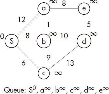
Figure 7-14: Starting conditions for finding the shortest paths from S
Node distances from the start node are given just outside the node circle. Nodes that haven’t been visited are assigned a tentative distance value of infinity (except for the start node, which has a value of zero). The queue shows the nodes with distance values indicated by exponents.
The first step is to pop the first node in the queue (which will always have a known distance) and color it with a light background as shown here in Figure 7-15. Set this node as the current node, u (in this case u = S with a distance value of zero).

Figure 7-15: Step 1 of Dijkstra’s algorithm
The neighbors of u are given in a darker color. We then perform the following tentative distance calculation, t, for each neighbor (designated v) of u that’s still in the queue, where d(u) is the known distance from the start node to u, and l(u, v) is the distance value of the edge from u to v:
If t is less than the prior distance value (initially ∞), the queue is updated with the new node distance.
With the queue updated, we repeat the process, this time popping c off the queue, making it the current node (in other words, u = c), and updating the queue and neighbor distances as before. The state of the graph is then as follows in Figure 7-16:

Figure 7-16: Step 2 of Dijkstra’s algorithm
We show the path from S to c in a thicker gray line to indicate a known shortest path in Figure 7-16. The sequence of diagrams in Figure 7-17 illustrates the remainder of the process. Notice that in Figure 7-17a the original distance of node a has been updated from 12 to 9 based on the path now being from S through b to a. The thick lines in 7-17d, the final graph, form a tree structure reflecting all the shortest paths originating from node S to the remaining nodes.

Figure 7-17: The rest of Dijkstra’s algorithm
We’re usually interested in how efficiently an algorithm performs. This is generally specified by a complexity value. There are a number of ways this can be done, but a popular formulation is called Big O notation (the O stands for “order of"). This notation aims to give a gross approximation of how efficiently an algorithm performs (in terms of running time or memory usage) based on the size of its inputs. Dijkstra’s algorithm has a running time complexity of O(N2), where N is the number of nodes in the graph. This means the running time increases as the square of the number of inputs. In other words, if we double the number of nodes, the algorithm will take about four times as long to run. This is taken to be an upper-bound or worst-case scenario, and depending on the nature of the graph, the runtime could be less.
The Priority Queue
As we’ve seen in the analysis above, a priority queue plays a key role in Dijkstra’s algorithm. Priority queues can be implemented in a number of ways, but one popular approach is to use something called a binary heap. A binary heap is a binary tree structure (meaning each node has a maximum of two children) where each node’s value is greater than or equal to its child nodes. This type of heap is called a max-heap. It’s also possible for each parent node to be less than or equal to its child nodes. This type of heap is called a min-heap. An example of such a heap is shown in Figure 7-18. The top or root node is always the first to be removed since it’s considered to have the highest priority. After nodes are added to or removed from the heap, the remaining nodes are rearranged to maintain the proper priority order. While it’s not terribly difficult to build a binary heap object, Racket already has one available in the data/heap library.
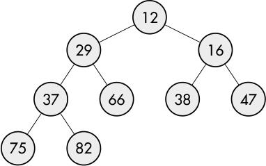
Figure 7-18: Min-heap
Our heap entries won’t be just numbers: we’ll need to track the node and its current distance value (which determines its priority). So each heap entry will consist of a pair where the first element is the node and the second element is the current distance. When a Racket heap is constructed, it must be supplied with a function that will do the proper comparison when given two node entries. We accomplish this with the following code. The comp function only compares the second element of each pair since that’s what determines the priority.
#lang racket
(require data/heap)

(define (comp n1 n2)
  (let ([d1 (cdr n1)]
        [d2 (cdr n2)])
    (<= d1 d2)))

(define queue (make-heap comp))
To save a bit of typing, we create a few simple helper functions.
(define (enqueue n) (heap-add! queue n))

(define (dequeue)
  (let ([n (heap-min queue)])
    (heap-remove-min! queue)
    n))

(define (update-priority s p)
  (let ([q (for/first ([x (in-heap queue)] #:when (equal? s (car x))) x)])
    (heap-remove! queue q)
    (enqueue (cons s p))))

(define (peek-queue) (heap-min queue))

(define (queue->list) (for/list ([n (in-heap queue)]) n))

(define (in-queue? s)
  (for/or ([x (in-heap queue)]) (equal? (car x) s)))
The update-priority procedure takes a symbol and a new priority to update the queue. It does this by removing (dequeuing) the old value and adding (enqueuing) a new value. The heap-remove! function performs very efficiently, but it needs the exact value (pair with symbol and priority) to work. Unfortunately, without knowing the priority, we have to resort to a linear search through the entire queue to find the symbol via the in-heap sequence. This can be optimized by storing (in another data structure like a hash table) the symbol and current priority. We leave it to the reader to perform this added step if desired.
Here are some examples of the priority queue in action.
> (enqueue '(a . 12))
> (enqueue '(b . 8))
> (enqueue '(c . 6))
> (queue->list)
'((c . 6) (b . 8) (a . 12))

> (in-queue? 'b)
#t

> (in-queue? 'x)
#f

> (update-priority 'a 9)
> (queue->list)
'((c . 6) (b . 8) (a . 9))

> (dequeue)
'(c . 6)

> (queue->list)
'((b . 8) (a . 9))

> (peek-queue)
'(b . 8)
Regardless of the order the values were added to the queue, they’re stored and removed in priority order.
The Implementation
We define our graph as a list of edges. Each edge in the list consists of the end nodes along with the distance between nodes.
(define edge-list
  '((S a 12)
    (S b 8)
    (S c 6)
    (a b 1)
    (b c 9)
    (a e 8)
    (e d 5)
    (b d 10)
    (c d 13)))
As we progress through the algorithm, we want to to keep track of the current parent of each node so that when the algorithm completes, we’ll be able to reproduce the shortest path to each node. A hash table will be used to maintain this information. The key is a node name and the value is the name of the parent node.
(define parent (make-hash))
We need to take care in our coding to be mindful of the fact that our graph is bi-directional, and an edge defined by (a, b) is equivalent to one defined by (b, a). We’ll account for this by supplementing the original edge list with a list consisting of the nodes reversed. We’ll also use a hash table (lengths) to maintain the lengths of each edge and an additional hash table (dist) to record the shortest distance to each node as it’s discovered. To pull all this together, we define init-graph, which takes an edge list and returns the original list appended with the swapped node list. It will also be used to initialize the priority queue and the various hash tables.
(define lengths (make-hash))
(define dist (make-hash))

(define (init-graph start-node edges)
  (let* ([INFINITY 9999]
         [swapped (map (λ (e) (list (second e) (first e) (third e))) edges)]
         [all-edges (append edges swapped)]
         [nodes (list->set (map (λ (e) (first e)) all-edges))])
    (hash-clear! lengths)
    (for ([e all-edges]) (hash-set! lengths (cons (first e) (second e)) (third e)))
    (set! queue (make-heap comp))
    (hash-clear! parent)
    (hash-clear! dist)
    (for ([n nodes])
      (hash-set! parent n null)
      (hash-set! dist n INFINITY)
      (if (equal? n start-node)
          (enqueue (cons start-node 0))
          (enqueue (cons n INFINITY))))
    (hash-set! dist start-node 0)
    all-edges))
Here’s the code, dijkstra, that actually computes the shortest paths for each node.
(define (dijkstra start-node edges)
  (let ([graph (init-graph start-node edges)])
 ➊ (define (neighbors n)
      (filter
       (λ (e) (and (equal? n (first e)) (in-queue? (second e))))
       graph))
 ➋ (let loop ()
      (let* ([u (car (dequeue))])
        (for ([n (neighbors u)])
       ➌ (let* ([v (second n)]
              ➍ [t (+ (hash-ref dist u) (hash-ref lengths (cons u v)))])
    ➎ (when (< t (hash-ref dist v))
           ➏ (hash-set! dist v t)
           ➐ (hash-set! parent v u)
           ➑ (update-priority v t)))))
   ➒ (when (> (heap-count queue) 0) (loop)))))
The dijkstra code takes the starting node symbol and edge list as arguments. It then defines graph, which is the original list of edges appended with a list of the edges with the nodes swapped. As mentioned, the init-graph procedure also initializes all the other data structures required for the algorithm to work. A local neighbors function is defined ➊ that takes a node and returns the list of nodes that are adjacent to the node and still in the queue. The main loop starts ➋ and the first step is to pop the first node in the queue and assign its symbol to u. Next, each of its neighbors (v) is processed ➌. For each neighbor, we compute t = d(u) + l(u, v) ➍ (recall that d(u) is the most current distance estimate from the start symbol to u, and l(u, v) is the length of the edge from u to v). We then test whether t < d(v) ➎, and if it passes the test, we do the following:
- Assign d(v) = t ➏.
- Assign u as the parent of v ➐.
- Update the queue with t as the new priority of v ➑.
Finally, we test whether any values remain on the heap, and if so, repeat the process ➒. Once the algorithm completes, parent will contain the parent of each node. All that remains is to chase the chain of parents to the start symbol to determine the shortest path to the node. This is done by the following get-path function:
(define (get-path n)
  (define (loop n)
    (if (equal? null n)
        null
        (let ([p (hash-ref parent n)])
          (cons n (loop p)))))
  (reverse (loop n)))
The show-paths procedure will print out paths for all the nodes.
(define (show-paths)
  (for ([n (hash-keys parent)])
    (printf "  ~a: ~a
" n (get-path n))))
For convenience we define solve, which takes a starting symbol and edge list, calls dijkstra to compute the shortest paths, and prints out the shortest path to each node.
(define (solve start-node edges)
  (dijkstra start-node edges)
  (displayln "Shortest path listing:")
  (show-paths))
Given our original graph where we defined the edges in edge-list above, and starting symbol S, we generate the solutions as follows:
> (solve 'S edge-list)
Shortest path listing:
  S: (S)
  e: (S b a e)
  a: (S b a)
  d: (S b d)
  c: (S c)
  b: (S b)
Let’s try this slightly more ambitious example in Figure 7-19 (see [4]).
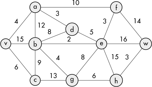
Figure 7-19: Another graph to test Dijkstra’s algorithm on
The edge list for this graph is . . .
> (define edges '((v a 4) (v b 15) (v c 6) (a b 12) (b c 9) (b d 8) (a f 10) (
     c v 6) (c g 13) (g h 6) (h w 3) (a d 3) (d e 5) (b e 2) (e w 16) (b g 4)
     (g e 8) (e h 16) (e f 3) (f w 14)))
So, solving for the shortest path, we have . . .
> (solve 'v edges)
Shortest path listing:
  d: (v a d)
  w: (v a d e b g h w)
  f: (v a f)
  c: (v c)
  v: (v)
  a: (v a)
  e: (v a d e)
  g: (v a d e b g)
  h: (v a d e b g h)
  b: (v a d e b)
We’ve highlighted the tree of shortest paths in the resulting graph (see Figure 7-20).

Figure 7-20: Shortest paths found
Now that we’ve thoroughly examined Dijkstra’s shortest-path algorithm, we’ll next take a look at the A* algorithm via Sam Loyd’s (in)famous 14–15 puzzle.
The 15 Puzzle
The 15 puzzle consists of 15 sequentially numbered sliding tiles in a square frame that are randomly scrambled, with the goal of getting them back into their proper numerical sequence. In the late 1800’s Sam Loyd created a bit of buzz over this puzzle by offering a $1,000 prize for anyone who could demonstrate a way to start with a puzzle with all the tiles in order, except with the 14 and 15 tiles reversed (as shown in Figure 7-21, Loyd called this arrangement the “14-15 Puzzle”), and get them back in their proper order (without removing the tiles from the case, of course). As we’ll see shortly, this is mathematically impossible, so Loyd knew his money was safe.
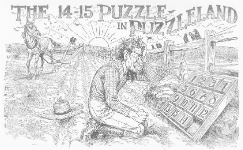
Figure 7-21: Sam Loyd’s 14–15 puzzle illustration
Why Swapping Just Two Tiles Is Impossible
To get an idea of why Loyd’s money was safe (that is, why it’s not possible to exchange two and only two tiles), consider the puzzle in its solved state as shown in Figure 7-22.

Figure 7-22: Solved 15 puzzle
Any sequence of moves that would reverse the 14 and 15 tiles would produce the arrangement in Loyd’s puzzle. Simply reproducing this sequence would get the tiles back in order. We’ll see that this is impossible. Now consider the arrangement in Figure 7-23.

Figure 7-23: 15 puzzle with inversions
If we arrange these tiles linearly, we have 2, 3, 1, 4, 5, 6, . . . In particular, the values of tile-2 and tile-3 are larger than tile-1, which follows them. Each such situation, where the value of a tile is larger than one that follows it, is called an inversion (two inversions in this case).
Related to the idea of inversion is that of transposition. A transposition is simply the exchange of two values in a sequence. A given arrangement can be arrived at by any number of transpositions. For example, one way to get to the sequence 2, 3, 1, 4, 5, 6, . . . would be as follows.
- Starting arrangement: 1, 2, 3, 4, 5, 6, . . .
- Transpose 1 and 3: 3, 2, 1, 4, 5, 6, . . .
- Transpose 2 and 3: 2, 3, 1, 4, 5, 6, . . .
The key idea is that an arrangement consisting of an even number of inversions will always be generated by an even number of transpositions, and an arrangement with an odd number of inversions will always be generated by an odd number of transpositions. For reference purposes, the empty slot will be treated as a tile and designated with the number 16. Any single movement by tile-16 is a transposition. If tile-16 leaves from the lower right corner and arrives at a particular spot using an odd number of transpositions, it will require an odd number of transpositions to get back to the starting location, or a net even number of transpositions. This leaves the puzzle with an even number of inversions.
The arrangement Sam Loyd proposes is impossible to solve since it involves a single odd inversion. It’s also true, but trickier to prove, that any puzzle with an even number of inversions is solvable.
Having resolved this historical issue with Sam Loyd’s puzzle, we now turn our attention to finding solutions for puzzles that are in fact solvable. In this regard we’ll now explore the A* search algorithm (we mostly abbreviate this to simply the “A* algorithm” hereafter).
The A* Search Algorithm
We’ll of course assume that the computer is presented with a solvable puzzle (that is, it has an even number of inversions). The computer should provide a solution that’s as efficient as possible—that is, a solution that requires the smallest number of moves to get to the goal state. One method that generally provides good results is called the A* search algorithm. An advantage of the A* algorithm over a simple breadth-first or depth-first search is that it uses a heuristic1 to reduce the search space. It does this by computing an estimated cost of taking any given branch in the search tree. It iteratively improves this estimate until it determines the best solution or it determines no solution can be found. Estimates are stored in a priority queue where the least cost state is at the head of the list.
We’ll begin our analysis by looking at a smaller variant of the 15 puzzle, called the 8 puzzle. The 8 puzzle in its solved state is shown in Figure 7-24.

Figure 7-24: Solved 8 puzzle
The search tree of the 8 puzzle can be modeled as shown in Figure 7-25, where each node of the tree is a state of the puzzle, and the child nodes are the possible states that can arise from a valid move.
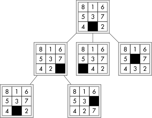
Figure 7-25: Partial 8 puzzle game tree
At each iteration of the A* algorithm, it computes an estimate of the cost (that is, the number of moves) to get to the goal state. Formally, it attempts to minimize the following estimated cost function, where n is the node under consideration, g(n) is the cost of the path from the start node to n, and h(n) is a heuristic that estimates the cost of the cheapest path from n to the goal:
f(n) = g(n) + h(n)
Designing a good heuristic function is something of an art. To get the best performance from the A* algorithm, an important characteristic of the heuristic is that it satisfies the following condition for every edge in the graph, where h*(n) is the actual (but unknown) cost to reach the goal state:
If a heuristic meets this condition, it’s said to be admissible, and the A* algorithm is guaranteed to find the optimal solution.
One possible heuristic for the 8 puzzle uses something called the Manhattan distance (as opposed to the familiar straight-line distance). For example, to get the tile-2 in Figure 7-25 to its home location (the cell it would occupy in the solved state), the tile would have to move up two squares and one square to the left for a total of three moves—this is the Manhattan distance. The heuristic value for a puzzle state would be the sum of the Manhattan distances for each tile. Table 7-1 shows the computation of this value for the root node of Figure 7-25.
Table 7-1: Computing Manhattan Distance
Tile |
Rows |
Cols. |
Total |
|---|---|---|---|
1 |
0 |
1 |
1 |
2 |
2 |
1 |
3 |
3 |
1 |
1 |
2 |
4 |
1 |
0 |
1 |
5 |
0 |
1 |
1 |
6 |
1 |
0 |
1 |
7 |
1 |
2 |
3 |
8 |
2 |
1 |
3 |
Distance: |
15 |
||
The Manhattan distance will always be less than or equal to the actual number of moves, so it satisfies the admissibility condition.
A slightly weaker heuristic is the Hamming distance, which is just the number of misplaced tiles. The Hamming distance for the puzzle shown in Figure 7-25 is eight: none of the tiles are in their home location.
In Figure 7-26 we’ve annotated each node with three values. The first value is the depth of the game tree (this value is incremented by one for each level and constitutes the value of g(n) in the cost formula), the second value is the heuristic value, h(n), for the node (the Manhattan distance in this case), and the third value is the sum of the two giving the overall cost score for the node.

Figure 7-26: 8 puzzle with node costs
The A* algorithm uses a priority queue called open. This queue orders the puzzle states that have been examined but whose child nodes have not been expanded, according to the estimated cost to reach the goal. The algorithm also relies on a dictionary, called closed, that uses the puzzle state as a key and maintains the most recent cost value for the node. Figure 7-27 reflects the current state of the analysis, where the first node in the open queue is the root node of Figure 7-26.

Figure 7-27: Closed and open
The values shown at the top of the closed nodes are the latest estimated costs. The values at the top of the open nodes are the same three cost values described above. With this introduction we walk through an iteration of how the A* algorithm processes the game tree.
The first step is to pop the lowest-priority value off the open queue. This node is then added to the closed dictionary. The next step is to compute the costs for the child nodes, which are shown on the second level of Figure 7-26. If any of these nodes are not on the closed list, they are simply queued to open with no further analysis. Notice that the first child node is on the closed list. Since its current estimated cost is less than the cost on the closed list, it’s removed from the closed list and the node is added back to the queue with its new value. In the situation where a child node is on the closed list, but its estimated value is larger than the value on the closed list, no change is made, and it’s not added to the queue. Once this phase is complete, the open and closed structures will appear as shown in Figure 7-28.
Since the first child node in Figure 7-26 has a lower cost than the other nodes in the open queue, it moves to the head of the queue and becomes the next item to be popped off. Notice that its first child is already in the closed list, but its newly computed cost is higher than the cost in the closed list, so it’s ignored. The remaining child node would be processed as before.

Figure 7-28: Closed and open, updated
The process continues until one of two things happens: either a node is popped off the open queue that’s in the solved state, in which case the algorithm completes and prints the answer (details on how this is accomplished are described in the next section), or the open queue becomes empty, which indicates that the puzzle was not solvable.
The 8-Puzzle in Racket
We’ll begin by implementing a solution to the smaller 3-by-3 version of the puzzle before we move on the full 4-by-4 version.
As with Dijkstra’s algorithm, we’ll use Racket’s heap object for the open priority queue:
#lang racket
(require data/heap)

(define (comp n1 n2)
  (let ([d1 (cdr n1)]
        [d2 (cdr n2)])
    (<= d1 d2)))

(define queue (make-heap comp))

(define (enqueue n) (heap-add! queue n))

(define (dequeue)
  (let ([n (heap-min queue)])
    (heap-remove-min! queue)
    n))
A SIZE constant will specify the number of rows and columns in the puzzle. In addition we’ll define a number of utility functions to work with the puzzle structure. For efficiency, the puzzle state will be stored internally as a Racket vector of size SIZE*SIZE+2. The last two elements of the vector will contain the row and column of the empty cell. The empty cell will have the numerical value specified by (define empty (sqr SIZE)). To this end, we have the following:
(define SIZE 3)
(define empty (sqr SIZE))

(define (ref puzzle r c)
  (let ([i (+ c (* r SIZE))])
    (vector-ref puzzle i)))

(define (empty-loc puzzle)
  (values
   (vector-ref puzzle empty)
   (vector-ref puzzle (add1 empty))))
The ref function will take a puzzle along with and a row and column number as arguments. It returns the tile number at that location. The empty-loc function will return two values that give the row and column respectively of the empty cell.
The following functions are used to compute the Manhattan distance. The first creates a hash table used to look up the home location of a tile given the tile number. The second function computes the sum of the Manhattan distances for each tile in the puzzle. This will be used in the computation of the cost of a puzzle node.
(define tile-homes
  (let ([hash (make-hash)])
    (for ([n (in-range (sqr SIZE))])
      (hash-set! hash (add1 n) (cons (quotient n SIZE) (remainder n SIZE))))
    hash))

(define (manhattan puzzle)
  (let ([dist 0])
    (for* ([r SIZE] [c SIZE])
      (when (not (= empty (ref puzzle r c)))
        (let* ([t (hash-ref tile-homes (ref puzzle r c))]
               [tr (car t)]
               [tc (cdr t)])
          (set! dist (+ dist
                        (abs (- tr r))
                        (abs (- tc c)))))))
    dist))
The next functions are used to generate a new puzzle state given a move specifier. A move specifier is a number from zero to three that determines which of the four directions a tile can be moved into the empty space from.
(define (move-offset i)
  (case i
    [(0) (values  0 -1)]
    [(1) (values  0  1)]
    [(2) (values -1  0)]
    [(3) (values  1  0)]))

(define (make-move puzzle i)
  (let*-values ([(ro co) (move-offset i)]
                [(re ce) (empty-loc puzzle)]
                [(rt ct) (values (+ re ro) (+ ce co))]
                [(t) (ref puzzle rt ct)])
    (for/vector ([i (in-range (+ 2 (sqr SIZE)))])
      (cond [(< i empty)
             (let-values ([(r c) (quotient/remainder i SIZE)])
               (cond [(and (= r re) (= c ce)) t]
                     [(and (= r rt) (= c ct)) empty]
                     [else (vector-ref puzzle i)]))]
            [(= i empty) rt]
            [else ct]))))
The move-offset function takes a move specifier and returns two values specifying the row and column deltas needed to make the move. The make-move function takes a move specifier and returns a new vector representing the puzzle after the move has been made.
The following function will take a puzzle and return a list consisting of all the valid puzzle states that can be reached from a particular puzzle state. The local legal function determines whether a move specifier will result in a valid move for the current puzzle state by checking whether a move in a certain direction will extend beyond the boundaries of the puzzle.
(define (next-states puzzle)
  (let-values ([(re ce) (empty-loc puzzle)])
    (define (legal i)
      (let*-values ([(ro co) (move-offset i)]
                    [(rt ct) (values (+ re ro) (+ ce co))])
        (and (>= rt 0) (>= ct 0) (< rt SIZE) (< ct SIZE))))
    (for/list ([i (in-range 4)] #:when (legal i))
      (make-move puzzle i))))
It will of course be useful to actually see a visual representation of the puzzle. That functionality is provided by the following routine.
(define (print puzzle)
  (for* ([r SIZE] [c SIZE])
    (when (= 0 c) (printf "
"))
    (let ([t (ref puzzle r c)])
      (if (= t empty)
          (printf "  ")
          (printf " ~a" t))))
  (printf "
"))
Next we define a helper function to process closed nodes.
(define closed (make-hash))

(define (process-closed node-parent node node-depth score)
  (begin
 ➊ (hash-set! closed node (list node-parent score))
    (for ([child (next-states node)])
   ➋ (let* ([depth (add1 node-depth)]
          ➌ [next-score (+ depth (manhattan child))]
          ➍ [next (cons (list child depth node) next-score)])
        (if (hash-has-key? closed child)
         ➎ (let* ([prior-score (second (hash-ref closed child))])
           ➏ (when (< next-score prior-score)
                (hash-remove! closed child)
                (enqueue next)))
         ➐ (enqueue next))))))
We begin by placing the node, its parent, and its estimated cost in the closed table ➊. Next, we generate a list of the possible child puzzle states and loop through them. For each child node, we generate the new node depth ➋ and estimated score ➌. Then we compile the information that we’d need to push that node to the open queue ➍, which happens automatically ➐ if the node is not in the closed table. If the node is in the closed table, we extract its prior cost score ➎ and compare with its current score ➏. If the current score is less than the prior score, we remove the node from the closed table and place it in the open queue.
We finally get to the algorithm proper.
(define (a-star puzzle)
  (let [(solved #f)]
    (hash-clear! closed)
 ➊ (set! queue (make-heap comp))  ; open
 ➋ (enqueue (cons (list puzzle 0 null) (manhattan puzzle)))
 ➌ (let loop ()
   ➍ (unless solved
        (let* ([node-info (dequeue)])
       ➎ (match node-info
            [(cons (list node node-depth node-parent) score)
          ➏ (if (= 0 (manhattan node))
                 (begin
                   (set! solved #t)
                   (print-solution (solution-list node-parent (list node))))
             ➐ (process-closed node-parent node node-depth score)
                 )])
       ➑ (if (> (heap-count queue) 0)
              (loop)
           ➒ (unless solved(printf "No solution found
"))))))))
First we define the closed hash table described above. The open queue is initialized ➊, and the scrambled puzzle provided to the a-star procedure is pushed onto the open queue ➋. The items in the queue consist of a Racket pair. The cdr of the pair is the estimated score, and the car consists of the puzzle state, the depth of the tree, and the parent puzzle state. After this initialization, the main loop starts ➌.
The loop repeats until the solved variable is set to true. The first step of the loop is to pop the highest-priority item (lowest cost score) from the open queue and assign it to the node-info variable. A match form is used to parse the values contained in node-info ➎. The puzzle state (in node) is first tested to see if it’s in the solved state ➏, and if so, the function prints out the move sequence and terminates the process. Otherwise, the processing continues where we process the closed node by placing the node, its parent, and estimated cost in the closed table ➐.
Once each iteration completes, the queue is checked ➑ to see if it contains any nodes that needs processing. If it does, then the next iteration resumes ➍; otherwise, no solution exists and the process terminates ➒.
Here are the print functions that show the solution. The solution-list procedure chases the parent nodes in closed to create a list of the puzzle states all the way back to the starting puzzle; print-solution takes the solution list and prints out the puzzle states it contains.
(define (solution-list n l)
  (if (equal? n null)
      l
      (let* ([parent (first (hash-ref closed n))])
        (solution-list parent (cons n l)))))

(define (print-solution l)
  (for ([p l]) (print p)))
Here’s a test run on the puzzle presented in Figure 7-25 (to save space, the output puzzles are displayed horizontally).
> (a-star #(8 1 6 5 3 7 4 9 2 2 1))

 8 1 6  8 1 6  8 1 6    1 6  1   6  1 3 6  1 3 6
 5 3 7  5 3 7    3 7  8 3 7  8 3 7  8   7    8 7
 4   2    4 2  5 4 2  5 4 2  5 4 2  5 4 2  5 4 2

 1 3 6  1 3 6  1 3 6  1 3 6  1 3 6  1 3 6  1 3 6
 5 8 7  5 8 7  5 8 7  5 8    5   8  5 2 8  5 2 8
   4 2  4   2  4 2    4 2 7  4 2 7  4   7  4 7

 1 3 6  1 3    1   3  1 2 3  1 2 3  1 2 3  1 2 3
 5 2    5 2 6  5 2 6  5   6    5 6  4 5 6  4 5 6
 4 7 8  4 7 8  4 7 8  4 7 8  4 7 8    7 8  7   8

 1 2 3
 4 5 6
 7 8
Moving Up to the 15 Puzzle
Having laid the groundwork with the 8 puzzle, the 15 puzzle requires this tricky modification: change the value of SIZE from 3 to 4. Okay, maybe that’s not too tricky, but before you get too excited, it’s really not quite that simple either. Observe Figure 7-29. The first two puzzles are from [9], and our test computer sailed through solving these. But the third puzzle was randomly generated and caused the test computer to fall to the floor, giggling to itself that we would attempt to have it solve such a problem—no solution was forthcoming.

Figure 7-29: Some 15 puzzle examples
The issue is that some puzzles may result in the A* algorithm having to explore too many paths, so the computer runs out of resources (or the user runs out of patience waiting for an answer). Our solution is to settle for a slightly less elegant approach by breaking the problem into three subproblems. We will trade off a fully optimized solution for a solution that we don’t have to wait forever to get.
To break the problem into subproblems, we’re going to divide the puzzle into three zones as shown below in Figure 7-30. The zones are chosen to take advantage of the fact that the A* algorithm was pretty zippy with the 8 puzzle.

Figure 7-30: 15 puzzle divided into zones
The medium gray section, which we designate zone 1, represents one subproblem, the white section (zone 2) will be the second subproblem, and the dark gray section (zone 3) represents another subproblem (which is equivalent to the 8 puzzle, which we know can be solved quickly). The idea is to provide different scoring functions to the a-star algorithm depending on which zone is being addressed. These functions will still use the Manhattan distance, but with certain restrictions applied. Once zone 1 and zone 2 have been solved, we can just call manhattan as before since the edge tiles in zones 1 and 2 will already be in place and the remaining tiles would be equivalent to an 8 puzzle.
Zone 1
Before we dive into solving zone 1, we’re going to create a helper function that’s quite similar to the code we saw in the manhattan function:
(define (cost puzzle guard)
  (let ([dist 0])
    (for* ([r SIZE] [c SIZE])
      (let ([t (ref puzzle r c)])
        (when (guard r c t)
          (let* ([th (hash-ref tile-homes t)]
                 [hr (car th)]
                 [hc (cdr th)]
                 [d (+ (abs (- hr r)) (abs (- hc c)))])
            (set! dist (+ dist d))))))
    dist))
The main difference is that instead of embedding the test for the empty square directly in the cost function, we’ll pass in a function for the guard parameter that will do the test for us. Given this, we can redefine manhattan as follows:
(define (manhattan puzzle)
  (cost puzzle (λ (r c t)
                 (not (= t empty)))))
We’ll attack zone 1 in two phases: first we nudge tiles 1 through 4 into the first two rows of the puzzle; then we get them into the proper order in the first row.
To get tiles 1 through 4 into the first two rows, we define zone1a.
(define (zone1a puzzle)
  (cost puzzle (λ (r c t)
                 (or (and (<= t 4) (> r 1))))))
In this case, we only update the distance for tiles 1 through 4, and we only update the distance if these tiles are not already in the first two rows.
The second phase is just slightly different. This time we always update the distance for tiles 1 through 4 to ensure they land in the proper locations.
(define (zone1b puzzle)
  (cost puzzle (λ (r c t)
                 (<= t 4))))
It might appear that this could have been done in a single function, but trying to position the tiles all at once would result in a large search space and the consequent increase needed in time and computer resources (like memory). Our first phase, where we just get the tiles into the proximity of their proper location, reduces the search space by half, without requiring an enormous amount of resources. The sorting in phase two will normally only have to deal with the tiles in the top half of the puzzles since the remaining tiles will have a score of zero.
Zone 2
At this point, we’ve reduced the search space by 25 percent. This modest reduction is sufficient to allow us to get tiles 5, 9, and 13 into zone 2 and in their proper order in a single procedure, which we provide here as zone2:
(define zone2-tiles (set 5 9 13))

(define (zone2 puzzle)
  (cost puzzle (λ (r c t)
                 (and (>= r 1)
                      (set-member? zone2-tiles t)))))
At this point, we no longer need to bother with row 1, as reflected in the code >= r 1. Aside from this, the code is nearly identical to the others, except that this time, we use the values defined in zone2-tiles for scoring.
Putting It All Together
Once a zone has been solved, we won’t want to disturb the tiles that are already in place. To accomplish this, a slight tweak is made to the function (next-states) that generates the list of permissible states. Before, we simply checked to ensure we weren’t moving beyond the first row or column. Now we define global variables min-r and min-c, which are set to 0 or 1 depending on which zone we’re currently working in.
(define min-r 0)
(define min-c 0)

(define (next-states puzzle)
  (let-values ([(re ce) (empty-loc puzzle)])
    (define (legal i)
      (let*-values ([(ro co) (move-offset i)]
                    [(rt ct) (values (+ re ro) (+ ce co))])
        (and (>= rt min-r) (>= ct min-c) (< rt SIZE) (< ct SIZE))))
    (for/list ([i (in-range 4)] #:when (legal i))
      (make-move puzzle i))))
The final solver will update the values of min-r and min-c once zones 1 and 2 have been populated.
We now need to make a few crucial modifications to the code for a-star and process-closed.
(define (process-closed node-parent node node-depth score fscore)
  (begin
    (hash-set! closed node (list node-parent score))
    (for ([child (next-states node)])
      (let* ([depth (add1 node-depth)]
          ➊ [next-score (+ depth (fscore child))]
             [next (cons (list child depth node) next-score)])
        (if (hash-has-key? closed child)
            (let* ([prior-score (second (hash-ref closed child))])
              (when (< next-score prior-score)
                (hash-remove! closed child)
                (enqueue next)))
            (enqueue next))))))
The most significant change is that instead of always using manhattan for our scoring estimate, we now use the function fscore ➊, which is passed to process-closed as an additional parameter. This function will be different depending on which zone of the puzzle is being solved.
(define (a-star puzzle fscore)
  (let ([solution null]
        [goal null])
    (hash-clear! closed)
    (set! queue (make-heap comp))  ; open
    (enqueue (cons (list puzzle 0 null) (fscore puzzle)))
    (let loop ()
      (when (equal? solution null)
        (let* ([node-info (dequeue)])
          (match node-info
            [(cons (list node node-depth node-parent) score)
             (if (= 0 (fscore node))
                 (begin
                ➊ (set! goal node)
                ➋ (set! solution (solution-list node-parent (list node))))
                 (process-closed node-parent node node-depth score fscore))])
          (if (> (heap-count queue) 0)
              (loop)
              (when (equal? solution null) (printf "No solution found
"))))))
 ➌ (values goal solution)))
Here we also include fscore as an additional parameter. Now, instead of immediately printing a solution once the goal state is reached, we return two values at the end ➌: the current goal, given in the first set! ➊ and the solution list, given in the second set! ➋. The remaining code should align closely with the original version.
Instead of calling a-star directly as we did before, we now provide a solve function that steps through the process of providing a-star with the proper scoring function, which is either one of the zone-specific functions or manhattan.
(define (solve puzzle)
  (set! min-r 0)
  (set! min-c 0)
  (let*-values ([(goal sol-z1a) (a-star puzzle zone1a)])
    (let*-values  ([(goal sol2) (a-star goal zone1b)]
                   [(sol-z1b) (cdr sol2)])
      (set! min-r 1)
      (let*-values  ([(goal sol3) (a-star goal zone2)]
                     [(sol-z2) (cdr sol3)])
        (set! min-c 1)
        (let*-values  ([(goal sol4) (a-star goal manhattan)]
                       [(sol-man) (cdr sol4)])
          (print-solution (append sol-z1a sol-z1b sol-z2 sol-man)))))))
As the code executes, it stores the solution list for each step of the process and finally prints the entire solution in the last line of the code. The reason we take the cdr of the solution list at each step (except the first) is because the last item in the solution from the previous step is the goal of the next step; this state would be repeated if we left it in the list.
Finally, we resolve a little cosmetic issue with the print routine caused by having two-digit numbers on the tiles. The revised code follows.
(define (print puzzle)
  (for* ([r SIZE] [c SIZE])
    (when (= 0 c) (printf "
"))
    (let ([t (ref puzzle r c)])
      (if (= t empty)
          (printf "   ")
          (printf " ~a" (~a t #:min-width 2 #:align 'right) ))))
  (printf "
"))
The following are some sample inputs with which to test the code. To save space, only the output (compressed) from the first example is shown.
> (solve #(2 10 8 3 1 6 16 4 5 9 7 11 13 14 15 12 1 2))

  2 10  8  3   2 10     3    2 10  3       2 10  3  4
  1  6     4   1  6  8  4    1  6  8  4    1  6  8
  5  9  7 11   5  9  7 11    5  9  7 11    5  9  7 11
 13 14 15 12  13 14 15 12   13 14 15 12   13 14 15 12

  2 10  3  4    2 10  3  4   2     3  4       2  3  4
  1  6     8    1     6  8   1 10  6  8    1 10  6  8
  5  9  7 11    5  9  7 11   5  9  7 11    5  9  7 11
 13 14 15 12   13 14 15 12  13 14 15 12   13 14 15 12

  1  2  3  4    1  2  3  4    1  2  3  4   1  2  3  4
    10  6  8    5 10  6  8    5 10  6  8   5     6  8
  5  9  7 11       9  7 11    9     7 11   9 10  7 11
 13 14 15 12   13 14 15 12   13 14 15 12  13 14 15 12

  1  2  3  4    1  2  3  4    1  2  3  4    1  2  3  4
  5  6     8    5  6  7  8    5  6  7  8    5  6  7  8
  9 10  7 11    9 10    11    9 10 11       9 10 11 12
 13 14 15 12   13 14 15 12   13 14 15 12   13 14 15

> (solve #(5 1 2 4 14 9 3 7 13 10 12 6 15 11 8 16 3 3))
. . .

> (solve #(10 9 5 13 8 14 15 7 1 3 11 6 4 2 12 16 3 3))
. . .

> (solve #(3 1 2 4 13 6 7 8 5 12 10 11 9 14 15 16 3 3))
. . .

> (solve #(9 6 12 3 5 13 16 8 14 1 10 7 2 15 11 4 1 2))
. . .

> (solve #(11 1 3 12 5 2 9 8 10 6 14 15 7 13 4 16 3 3))
. . .
Be aware that depending on the puzzle and the power of your computer, it may take anywhere from a couple of seconds to a minute or so to generate a solution.
Sudoku
Sudoku2 is a popular puzzle consisting of a 9-by-9 grid of squares in which some squares are initially populated with digits from 1 through 9, as shown in Figure 7-31a. The objective is to fill in the blank squares such that each row, column, and 3-by-3 block of squares also consists of digits 1 through 9, as shown in Figure 7-31b. A well-formed Sudoku puzzle should only have one possible solution.

Figure 7-31: The Sudoku puzzle
Our aim in this section is to produce a procedure that generates the solution to any given Sudoku puzzle.
The basic strategy is this:
- Check each empty cell, to determine which numbers are available to be used.
- Select a cell with the fewest available numbers.
- One at a time, enter one of the available numbers in the cell.
- For each available number, repeat the process until either the puzzle is solved, or there are no numbers available for an empty cell.
- If there are no available numbers, backtrack to step 3 and try a different number.
The process is another application of depth-first search.
Figure 7-32 gives the coordinates used to reference locations in the puzzle: numbers across the top index columns, numbers on the left edge index rows, and numbers in the interior index blocks of 3-by-3 subgrids.

Figure 7-32: Puzzle coordinates
To determine the available numbers for a given cell, we take the set intersection of the unused numbers in each row, column, and block. Using the cell in row 1, column 1 of Figure 7-31a as an example, in row 1 the set of numbers {2, 5, 8} are free, in column 1 all the numbers except for 5 are available, and in block 0, the set of numbers {2, 3, 7, 8, 9} are available. The intersection of these sets gives the set of possible values for this cell: {2, 8}.
Our implementation will use a 9-by-9 array of numbers to represent the puzzle, where the number 0 will designate an empty square. The array will be constructed of a nine-element vector, each element being another nine-element integer vector. For easy access to elements of the array, we define two utility functions to set and retrieve values:
(define (array-set! array r c v)
  (vector-set! (vector-ref array r) c v))

(define (array-ref array r c)
  (vector-ref (vector-ref array r) c))
Both of these functions require the array and row and column numbers to be provided as the initial arguments.
It will also be useful to derive the corresponding block index from the row and column numbers, as given by the getBlk function here.
(define (getBlk r c) ; block from row and column
  (+ (* 3 (quotient r 3)) (quotient c 3)))
The puzzle will be input as a single string where each row of nine digits is broken by a new line as shown by the example below.
> (define puzzle-str "
150000320
604031097
000200000
000049073
400800000
000000001
503008000
002000004
007000260
")
We define the Sudoku puzzle object as a sudoku% Racket object for which we give a partial implementation here. This object will maintain the puzzle state. It will contain functions that allow us to manipulate the state by setting cell values and provides functions to list potential candidates (unused numbers in a row, column, or block) and other helper functions.
(define sudoku%
  (class object%

 ➊ (init [puzzle-string ""])

    (define avail-row (make-markers))
    (define avail-col (make-markers))
    (define avail-blk (make-markers))
 ➋ (define count 0)

 ➌ (define grid
      (for/vector ([i 9]) (make-vector 9 0)))

    (super-new)

 ➍ (define/public (item-set! r c n)
      (array-set! grid r c n)
      (array-set! avail-row r n #f)
      (array-set! avail-col c n #f)
      (let ([b (getBlk r c)])
        (array-set! avail-blk b n #f))
      (set! count (+ count 1)))
    (unless (equal? puzzle-string "")
   ➎ (init-puzzle puzzle-string))

    (define/public (get-grid) grid)

    (define/public (item-ref r c)
      (array-ref grid r c))

 ➏ (define/public (init-grid grid)
      (for* ([r 9] [c 9])
        (let ([n (array-ref grid r c)])
          (when (> n 0)
            (item-set! r c n)))))

 ➐ (define/private (init-puzzle p)
      (let ([g
             (let ([rows (string-split p)])
               (for/vector ([row rows])
                 (for/vector ([c 9])
                   (string->number (substring row c (add1 c))))))])
        (init-grid g)))

; More to come shortly . . .

))
The init form ➊ captures the input string value that defines the puzzle. We initialize the puzzle ➎ by calling init-puzzle ➐, which updates grid ➌ with the appropriate numerical values via the call to init-grid ➏.
The count variable ➋ contains the number of cells that currently have a value. Once count reaches 81, the puzzle has been solved.
The avail-row, avail-col, and avail-blk variables are used to keep track of which numbers are currently unused in each row, column, and block respectively. The make-markers function, which is called to initialize each of these variables, creates a Boolean array that indicates which numbers are free for any given index (row, column, or block as applicable); make-markers is defined as follows:
(define (make-markers)
  (for/vector ([i 10])
    (let ([v (make-vector 10 #t)])
      (vector-set! v 0 #f)
      v)))
Notice that the number 0 (designating an empty cell) is automatically marked as unavailable.
As numbers get added to the puzzle, item-set! is called ➍. This procedure is responsible for updating grid and avail-row, avail-col, and avail-blk when given the row, column, and number to be assigned to the puzzle. The functions get-grid and item-ref return grid or a cell in grid respectively.
In the following code extracts, all function definitions that are indented should be included in the class definition for sudoku% and aren’t global defines.
The following avail function combines the values from avail-row, avail-col, and avail-blk to produce a vector indicating which numbers are available.
    (define (avail r c)
      (let* ([b (getBlk r c)]
             [ar (vector-ref avail-row r)]
             [ac (vector-ref avail-col c)]
             [ab (vector-ref avail-blk b)])
        (for/vector ([i 10])
          (and (vector-ref ar i)
               (vector-ref ac i)
               (vector-ref ab i)))))
Given this vector, we create a list of the free numbers as follows:
    (define (free-numbers v)
      (for/list ([n (in-range 1 10)] #:when (vector-ref v n)) n))
For efficiency, the following code finds all the cells that only have a single available number and updates the puzzle appropriately.
    (define (set-singles)
      (let ([found #f])
        (for* ([r 9] [c 9])
          (let* ([free (avail r c)]
                 [num-free (vector-count identity free)]
                 [n (item-ref r c)])
            (when (and (zero? n)  (= 1 num-free))
              (let ([first-free
                     (let loop ([i 1])
                       (if (vector-ref free i) i
                           (loop (add1 i))))])
                (item-set! r c first-free)
                (set! found #t))
              )))
        found))
Performing this process once may result in other cells with only a single available number. The following code runs until no cells remain with only a single available number.
    (define/public (set-all-singles)
      (when (set-singles) (set-all-singles)))
For puzzles that can be solved directly by logic alone (no guessing is required), the above process would be sufficient, but this isn’t always the case. To support backtracking, the following two functions are provided.
    (define (get-free)
      (let ([free-list '()])
        (for* ([r 9] [c 9])
          (let* ([free (avail r c)]
                 [num-free (vector-count identity free)]
                 [n (item-ref r c)])
            (when (zero? n)
              (set! free-list
                    (cons
                     (list r c num-free (free-numbers free))
                     free-list)))))
        free-list))

    (define/public (get-min-free)
      (let ([min-free 10]
            [min-info null]
            [free-list (get-free)])
        (let loop ([free free-list])
          (unless (equal? free '())
            (let* ([info (car free)]
                   [rem (cdr free)]
                   [num-free (third info)])
              (when (< 0 num-free min-free)
                (set! min-free num-free)
                (set! min-info info))
              (loop rem))))
        min-info))
The first function (get-free) goes cell by cell and creates a list of all the free values for each cell. Each element of the list contains another list that holds the row, column, number of free values, and a list of the free values. The second function (get-min-free) takes the list returned by get-free and returns the values for the cell with the fewest free numbers.
Here are a few handy utility functions.
    (define/public (print)
      (for* ([r 9] [c 9])
        (when (zero? c) (printf "
"))
        (let ([n (item-ref r c)])
          (if (zero? n)
              (printf " .")
              (printf " ~a" n)
              )))
      (printf "
"))

    (define/public (solved?) (= count 81))

    (define/public (clone)
      (let ([p (new sudoku%)])
        (send p init-grid grid)
        p))
The print member function provides a simple text printout of the puzzle. The solved? function indicates whether the puzzle is in the solved state by testing whether all 81 cells have been populated. The clone function provides a copy of the puzzle.
This concludes the code that’s defined within the body of the sudoku% class definition and brings us to the actual code used to solve the puzzle.
(define (solve-sudoku puzzle)
  (let ([solution null]
     ➊ [puzzle (send puzzle clone)])
 ➋ (define (dfs puzzle)
      (if (send puzzle solved?)
          (set! solution puzzle)
          (let ([info (send puzzle get-min-free)])
            (match info
              ['() #f]
           ➌ [(list row col num free-nums)
               (let loop ([nums free-nums])
                 (if (equal? nums '())
                     #f
                  ➍ (let ([n (car nums)]
                        ➎ [t (cdr nums)])
                       (let ([p (send puzzle clone)])
                      ➏ (send p item-set! row col n)
                         (send p set-all-singles)
                      ➐ (unless (dfs p)(loop t))))))]))))
 ➑ (send puzzle set-all-singles)
    (dfs puzzle)
    (if (equal? solution null)
        (error "No solution found.")
        solution
        )))
We begin by creating a copy of the puzzle to work with ➊. Next, we define a depth-first search procedure, dfs ➋, which we’ll explain shortly. The call to set-all-singles ➑ is occasionally sufficient to solve the puzzle, but the puzzle is handed off to dfs to ensure a complete solution is found. The remaining lines will return a solved puzzle if one exists; otherwise an error is signaled.
The depth-first search code, dfs ➋, immediately tests whether the puzzle is solved and if so, returns the solved puzzle. Otherwise, the cell with the fewest available numbers (if any) is explored ➌, where the match form extracts the cell row, column, number of free numbers, and the list of free numbers. The list of free numbers is iterated through starting on the next line. While the list isn’t empty, the first number in the list is extracted into n ➍ and the remaining numbers are stored in t ➎. Then a copy of the puzzle is created. Next, the puzzle copy is populated with the current available number ➏, and set-all-singles is called immediately following this. If this number doesn’t produce a solution (via the recursive call to dfs ➐), the loop repeats with the original puzzle and the next available number.
To aid testing various puzzles, we define a simple routine to take an input puzzle string, solve the puzzle, and print the solution.
(define (solve pstr)
  (let* ([puzzle (new sudoku% [puzzle-string pstr])]
         [solution (solve-sudoku puzzle)])
    (send puzzle print)
    (send solution print)))
Now that we’ve laid this groundwork, here’s a trial run with our example puzzle.
> (define puzzle "
150000320
604031097
000200000
000049073
400800000
000000001
503008000
002000004
007000260
")
> (solve puzzle)

 1 5 . . . . 3 2 .
 6 . 4 . 3 1 . 9 7
 . . . 2 . . . . .
 . . . . 4 9 . 7 3
 4 . . 8 . . . . .
 . . . . . . . . 1
 5 . 3 . . 8 . . .
 . . 2 . . . . . 4
 . . 7 . . . 2 6 .

 1 5 8 9 7 4 3 2 6
 6 2 4 5 3 1 8 9 7
 7 3 9 2 8 6 1 4 5
 2 8 5 1 4 9 6 7 3
 4 7 1 8 6 3 9 5 2
 3 9 6 7 5 2 4 8 1
 5 6 3 4 2 8 7 1 9
 8 1 2 6 9 7 5 3 4
 9 4 7 3 1 5 2 6 8
While this is certainly an adequate method to generate the output, it doesn’t take a lot of additional work to produce a more attractive output.
To accomplish our goal, we’ll need the Racket draw library.
(require racket/draw)
Furthermore, we’ll borrow our draw-centered-text procedure that we used in the 15 puzzle GUI:
(define CELL-SIZE 30)

(define (draw-centered-text dc text x y)
  (let-values ([(w h d s) (send dc get-text-extent text)])
    (let ([x (+ x (/ (- CELL-SIZE w) 2))]
          [y (+ y (/ (- CELL-SIZE h d) 2))])
      (send dc draw-text text x y ))))
Given these preliminaries, we can now define our draw-puzzle function:
(define (draw-puzzle p1 p2)
  (let* ([drawing (make-bitmap (* 9 CELL-SIZE) (* 9 CELL-SIZE))]
         [dc (new bitmap-dc% [bitmap drawing])]
         [yellow (new brush% [color (make-object color% 240 210 0)])]
         [gray (new brush% [color "Gainsboro"])])
    (for* ([r 9][c 9])
      (let* ([x (* c CELL-SIZE)]
             [y (* r CELL-SIZE)]
             [n1 (send p1 item-ref r c)]
             [n2 (send p2 item-ref r c)]
             [num (if (zero? n2) "" (number->string n2))]
             [color (if (zero? n1) yellow gray)])
        (send dc set-pen "black" 1 'solid)
        (send dc set-brush color)
        (send dc draw-rectangle x y CELL-SIZE CELL-SIZE)
        (draw-centered-text dc num x y)))
    (for* ([r 3][c 3])
      (let* ([x (* 3 c CELL-SIZE)]
             [y (* 3 r CELL-SIZE)])
        (send dc set-pen "black" 2 'solid)
        (send dc set-brush "black" 'transparent)
        (send dc draw-rectangle x y (* 3 CELL-SIZE) (* 3 CELL-SIZE))))
    drawing))
There’s really nothing new here. The reason we’re passing it two puzzles is because the first puzzle is the original unsolved puzzle. It’s simply used to determine which color to use to draw the squares. If a square was blank in the original puzzle, it’ll be colored yellow in the output; otherwise it’ll be colored gray.
With this in hand, we can redefine solve as follows:
(define (solve pstr)
  (let* ([puzzle (new sudoku% [puzzle-string pstr])]
         [solution (solve-sudoku puzzle)])
    (print (draw-puzzle puzzle puzzle))
    (newline)
    (newline)
    (print (draw-puzzle puzzle solution))))
Using this new version yields the following:
> (solve "
150000320
604031097
000200000
000049073
400800000
000000001
503008000
002000004
007000260
")
It gives the starting state in Figure 7-33:
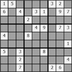
Figure 7-33: Sudoku starting-state drawing
And the solved state in Figure 7-34:
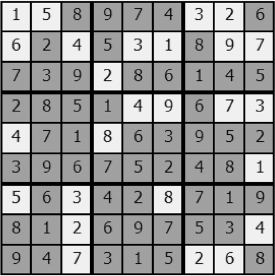
Figure 7-34: Solved Sudoku drawing
Summary
In this chapter, we’ve explored a number of algorithms that are useful in the general context of problem-solving. In particular we’ve looked at breath-first search (BFS), depth-first search (DFS), the A* algorithm, and Dijkstra’s algorithm (and discovered priority queues along the way) to find the shortest path between graph nodes. We employed DFS in the solution of the n-queens problem and the 15 puzzle (which also used the A* algorithm). Finally, we took a look at Sudoku, where sometimes logic alone is sufficient to solve, but failing this, DFS again comes to the rescue. While the algorithms we’ve explored are far from a comprehensive set, they form a useful toolset that’s effective in solving a wide range of problems over many domains.
Thus far we’ve exercised a number of programming paradigms: imperative, functional, and object-oriented. In the next chapter, we’ll look at a new technique: programming in logic or logic programming.