9
COMPUTING MACHINES

We’re all used to having access to powerful computing devices with complex architectures and instruction sets, but fundamental ideas of computer science are based on far simpler devices. The basic idea is to begin with the simplest possible devices and determine what types of computations are possible. We’ll explore three such devices below, ranging from ones that can only perform simple operations like recognizing strings to ones that can carry out any algorithm.

Finite-State Automata

In this section, we’ll introduce an abstract machine—a computational model, not a physical machine—called a finite-state automaton (FSA) or finite-state machine (FSM). In spite of its impressive name, a finite-state automaton is really something very simple. The entire raison d’être of finite-state automata is to execute conditional expressions.

An FSA has a (metaphorical) tape with a series of symbols as inputs. Each symbol is read exactly once, and the machine then moves to the next symbol in the sequence. An FSM is modeled using a finite number of states and transitions, hence the name finite-state machine. The machine starts in a given initial state and transitions to another state based on the input symbol. It can exist in exactly one state at any given time. Some of the states are accepting states, and if the machine finishes in an accepting state, the input string is valid. It’s possible that, depending on the input and possible transitions from a state, the machine can’t continue, in which case the string is invalid. The key is that for every input, there’s a condition for each transition.

Finite-state automata can be used to model many different types of computations, but in this section, we’ll focus on their popular use in computer science as recognizers: programs that, given an input string, indicate whether the sequence is valid or invalid. As an example, we’ll look at a recognizer that will accept strings of the form “HELLO,” “HELLLO,” “HELLOOO,” and so on, and reject all other strings. It’s clear from the nature of this problem that not only does an FSA need to be able to perform computations conditionally, but repetition (and hence, iteration) also comes into play.

There are a number of different ways to represent an FSM program; we’ll employ two of them: a state-transitions diagram and a state table. A state-transitions diagram is a directed graph that describes how the FSM transitions from one state to the next. Each state is indicated by a circle. The initial state is identified by an arrow pointing to one of the states, and the accepting states (there can be more than one) are usually indicated by double circles. States are connected by lines or arcs, each of which is labeled with an input symbol. The FSM transitions from one state to the next based on whether the current input symbol matches the label on one of its exiting arcs. A string is said to be accepted if it eventually reaches one of the accepting states; otherwise, it’s rejected.

An FSM for recognizing our “HELLO” strings is shown in Figure 9-1.

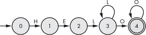
Figure 9-1: An FSM for “HELLO” strings

The FSM begins in state 0, and when it receives an “H” for input, it moves to state 1; otherwise, it halts at state 0 (indicating a rejected string). Once in state 1, it expects an “E” and accepts or rejects the input value as before. It proceeds in this fashion until it reaches the final accepting state (state 4). Observe that state 3 can accept either an “L” or an “O.” An FSM, such as this one, built in such a way that every state has only a single transition for each input symbol, is called a deterministic FSM (or a DFA). It’s possible to build finite-state automata where one or more states may transition to more than one state for the same input symbol. Such an FSM is called a nondeterministic FSM (or an NFA). For any nondeterministic FSM, we can construct a deterministic FSM so they’re both capable of recognizing the same set of strings. The advantage of nondeterministic FSMs is that in some cases, they’re simpler than their deterministic counterparts. In this text, we’ll only be using deterministic finite-state machines.

We can also represent our FSM as a state table (sometimes called an event table). See Table 9-1. The first column of the table contains the state number, and the remaining columns represent the input symbols. The table cells contain the next state for a given input symbol. If no state is given, the input symbol is rejected.

Table 9-1: State Table for "HELLO" Strings

S	H	E	L	O
0	1
1		2
2			3
3			3	4
4				4

To implement an FSM to recognize our “HELLO” strings in Racket, we first define a state table as follows:

#lang racket

(define state-table
  (vector
   ;        H  E  L  O
   (vector  1 #f #f #f) ; state 0
   (vector #f  2 #f #f) ; state 1
   (vector #f #f  3 #f) ; state 2
   (vector #f #f  3  4) ; state 3
   (vector #f #f #f  4) ; state 4
   ))

In this case, we’re using #f to indicate an invalid transition.

Since we’re using vectors for our state table, we need a way to convert characters to indexes. This is done with a hash table, as shown in the following definition.

(define chr->ndx
  (make-hash '[(#H . 0) (#E . 1) (#L . 2) (#O . 3)] ))

Given a state number and character, the following next-state function gives the next state (or #f) from the state table.

(define (next-state i chr)
  (if (hash-has-key? chr->ndx chr)
      (vector-ref (vector-ref state-table i)
                  (hash-ref chr->ndx chr) )
      #f))

Finally, here’s the DFA to recognize our “HELLO” strings.

  (define (hello-dfa str)
➊ (let ([chrs (string->list str)])
    (let loop ([state 0] [chrs chrs])
   ➋ (if (equal? chrs '()) ; end of string
       ➌ (if (= state 4) 
              #t ;if 4, accepting
              #f ;not 4, not accepting
              )
       ➍ (let ([state (next-state state (car chrs))]
                [tail (cdr chrs)])
            (if (equal? state #f) #f ; invalid
             ➎ (loop state tail)))))))

First, we convert our string to a list of characters ➊. Then we loop on this list, first checking to see whether all the characters have been read ➋. We then check the state ➌. If we’re in an accepting state (in this case, state 4), we return #t indicating an accepted string; otherwise, we return #f. If the entire string hasn’t been processed, we get the next state and the rest of the string ➍. We then start the process over again with the remainder of the string ➎. Here are a few sample runs.

> (hello-dfa "HELP")
#f

> (hello-dfa "HELLO")
#t

> (hello-dfa "HELLLLLOOOO")
#t

> (hello-dfa "HELLOS")
#f

It turns out that finite-state automata (both deterministic and nondeterministic) have certain limitations. For example, it’s not possible to build a finite-state machine that recognizes matching parentheses (since at any point, we would need a mechanism to remember how many open parentheses had been encountered). In the next section, we’ll introduce the FSM’s smarter brother, the Turing machine.

The Turing Machine

The Turing machine is an invention of the brilliant British mathematician Alan Turing. In its simplest form, a Turing machine is an abstract computer that consists of the following components.

• An infinite tape of cells that can contain either a zero or a one (arbitrary symbols are also allowed, but we don’t use them here)
• A head that can read or write a value in each cell and move left or right (see Figure 9-2)
• A state table
• A state register that contains the current state

Figure 9-2: Turing machine tape and head

Despite this apparent simplicity, given any computer algorithm, a Turing machine can be constructed that’s capable of simulating that algorithm’s logic. Conversely, any computing device or programming language that can simulate a Turing machine is said to be Turing complete. Thus, a Turing machine is not hampered by the limitations we mentioned for finite-state automata. There’s a large body of literature where the Turing machine plays into the analysis of whether certain functions are theoretically computable. We won’t engage in these speculations, but rather concentrate on the basic operation of the machine itself.

The machine we construct will have the simple task of adding two numbers. A number, n, will be represented as a contiguous string of n ones. The numbers to be added will be separated by a single zero, and the head will be positioned at the leftmost one of the first number. The result will be a string of ones, whose length will be the sum of the two numbers. At the end of the computation, the head will be positioned at the leftmost one of the result.

In a nutshell, the program works by changing the leftmost one of the leftmost number to zero, then scanning to the right until it reaches the end of the second number and writing a one just after the last one. The head then moves to the left until one of two things happens:

• It encounters a zero followed by a one, which means there are more ones left to move, so it continues to the left so that it can start over.
• It encounters two consecutive zeros, in which case the addition is done (because there are no other ones left from the first number), and it moves to the right until it is positioned over the leftmost one of the final number.

Figure 9-3 contains some snapshots of the tape at various times during the computation (the triangle shows the head at the start and end of the computation).

Figure 9-3: The tale of the tape

You may have already figured out that there are more direct ways to combine the two strings of numbers, but the method described lends itself to being adapted to other computations like multiplication.

Programming a Turing machine consists of constructing a state table. Each row in the table represents a particular state. Each state specifies three actions depending on whether the head currently reads a zero or a one. The actions will be to either write a one or a zero to the current cell, whether to move left or right afterward, and what the next state should be. Table 9-2 contains our adder program.

Table 9-2: Turing Machine State Table

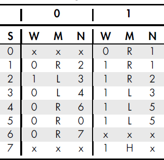
The topmost row indicates the input symbol. The columns labeled with a W indicate the value that should be written, the columns headed by an M indicate the direction to move (left or right), and the columns headed by an N indicate the next state number. Entries marked with an x are states that will never be reached (this is assuming the inputs and start state are properly set)—in such cases, the entries would be irrelevant. The machine starts in state 0. The final state (or halting state) is state 7, indicted by an H in the move column for a one input.

An alternative (and possibly easier-to-decipher) method of representing a Turing machine’s state changes is with a state-transition diagram, as shown in Figure 9-4. In the state diagram, each transition label has three components: the symbol being read, the symbol to write, and the direction to move.

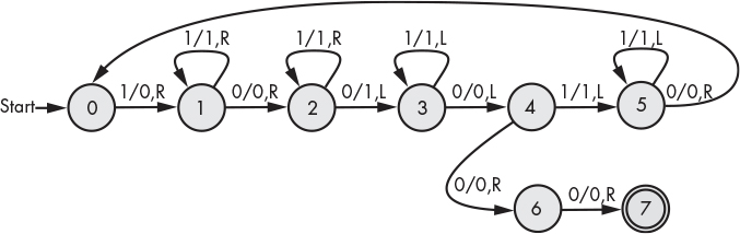
Figure 9-4: Turing machine state-transition diagram

A Racket Turing Machine

As mentioned at the beginning of this section, a programming language that can simulate a Turing machine is said to be Turing complete. We’ll demonstrate that Racket is itself Turing complete by constructing just such a simulation (using our addition machine as an example program). We’ll of course have to compromise a bit on the infinite tape, so our machine will have a more modest tape, with just 10 cells. The state table will consist of a vector where each cell represents a state. Each state is a two-cell vector where the first cell consists of the actions when a zero is read, and the second cell consists of the actions when a one is read. The actions will be represented by a structure called act. The act structure will have fields write, move, and next (with obvious meanings). The state will be given in a variable called state, and the position of the head will be in head. Given these initial considerations, we have the following:

#lang racket

(define tape (vector 1 1 1 0 1 1 0 0 0 0))

(define head 0)

(struct act (write move next))

(define state-table
  (vector
   (vector (act 0 #f 0) (act 0 'R 1)) ; state 0
   (vector (act 0 'R 2) (act 1 'R 1)) ; state 1
   (vector (act 1 'L 3) (act 1 'R 2)) ; state 2
   (vector (act 0 'L 4) (act 1 'L 3)) ; state 3
   (vector (act 0 'R 6) (act 1 'L 5)) ; state 4
   (vector (act 0 'R 0) (act 1 'L 5)) ; state 5
   (vector (act 0 'R 7) (act 1 #f 0)) ; state 6
   (vector (act 0 #f 0) (act 1 'H 0)) ; state 7
   ))
  
(define state 0)

While not strictly required by the definition, we’ve included an #f value (indicating fail) in the “don’t care” states just in case there was some error introduced in the initial setup of the problem (hey, nobody’s perfect).

Before getting to the code that specifies the machine’s execution, we define a few helper functions to get at various components. The first function returns the next state given the current state and input symbol, and the other two get and set the value at the tape head.

(define (state-ref s i) (vector-ref (vector-ref state-table s) i))
(define (head-val) (vector-ref tape head))
(define (tape-set! v) (vector-set! tape head v))

The program for running the machine is straightforward. Note that this code is the same for any Turing machine you program; only the tape and state-table change.

(define (run-machine)
  (let* ([sym (head-val)] ; current input
      ➊ [actions (state-ref state sym)]
         [move (act-move actions)])
    (cond [(equal? #f move)
           (printf "Failure in state ~a, head: ~a
~a" state head tape)]
       ➋ [(equal? 'H move)
           (printf "Done!
")]
          [else
        ➌ (let* ([write (act-write actions)]
               ➍ [changed (not (equal? sym write))])
             (tape-set! write)
          ➎ (set! head (if (equal? move 'L) (sub1 head) (add1 head)))
          ➏ (when changed (printf "~a
" tape))
          ➐ (set! state (act-next actions))
             (run-machine))])))

First we capture the actions for the current state and input ➊. Then we capture the next symbol to write ➌ and update the next state ➐. We also test whether the head is about to change a value on the tape ➍, in which case we print out the updated tape ➏. The head position is updated earlier ➎. Once the final state is reached ➋, the program will print Done!. Here’s the output.

#(1 1 1 0 1 1 0 0 0 0)
#(0 1 1 0 1 1 0 0 0 0)
#(0 1 1 0 1 1 1 0 0 0)
#(0 0 1 0 1 1 1 0 0 0)
#(0 0 1 0 1 1 1 1 0 0)
#(0 0 0 0 1 1 1 1 0 0)
#(0 0 0 0 1 1 1 1 1 0)
Done!

Pushdown Automata

The phrase “pushdown automata” is not a call to go out and knock over un-suspecting robots. No, the term pushdown automaton (or PDA) refers to a class of abstract computing devices that use a pushdown stack (or just stack to friends). In terms of computing power, pushdown automata lie squarely between that of finite-state automata and Turing machines.

The advantage of a PDA over a finite-state automaton lies in the stack. The stack forms a basic type of memory. Conceptually, a stack is like a stack of plates where you’re only allowed to remove a plate from the top of the stack (called a pop) or add (push) a plate to the top. The rest of the stack can only be accessed via adds or removes from the top. To simulate this in Racket, we define a stack as a string of symbols with two operations:

• Push. This operation adds a symbol to the top of the stack (front of the string).
• Pop. Pop removes the symbol at the top of the stack and returns it.

A PDA is allowed to read the top symbol on the stack, but it has no access to other stack values. Stack values don’t necessarily have to match the values used as input symbols.

Like an FSA, a PDA sequentially reads its input and uses state transitions to determine the next state, but a PDA has the requirement that in addition to being in an accepting state, the stack must also be empty for a string to be accepted (but for practical purposes, in the example below we pre-populate the stack with a unique marker to indicate an empty stack). Be aware that pushdown automata come in deterministic and nondeterministic varieties. Further, nondeterministic pushdown automata are capable of performing a wider range of computations.

While we generally try to keep the presentation informal, we’re going to provide a formal description of a PDA since you’re likely to run across this type of notation if you elect to do further research on abstract computing machines.¹ If you’re not familiar with set notation, you may want to jump to “Set Theory” in Chapter 4 to brush up.

Generally, a PDA is defined as a machine M = (Q, Σ, Γ, q₀, Z, F, δ), where the following is true:

• Q is a finite set of states.
• Σ is the set of input symbols.
• Γ is the set of possible stack values.
• q₀ ∈ Q is the start state.
• Z ∈ Γ is the initial stack symbol.
• F ⊆ Q is the set of accepting states.
• δ is the set of possible transitions.

The set of permissible transitions are then defined by this somewhat intimidating expression (where Γ^* is used to designate all the possible stack strings, and the symbol ϵ is used to represent the empty string, a string with no symbols in it).

δ ⊆ (Q × (Σ ∪ {ϵ}) × Γ) × (Q × Γ*)

This isn’t as bad as it looks. It’s basically saying that the set of possible transitions is a subset of all possible combinations of states, input symbols, and stack values (that is, all possibilities pre-transition) with all possible states and stack strings (the possibilities post-transition). The first set of values in parentheses represents inputs to the transition function and consists of the following:

• the currents state: q ∈ Q
• the current input symbol: i ∈ (Σ ∪ {ϵ}) (remember that we use ϵ to indicate that the remaining string can be empty at some point)
• the value at the top of the stack: s ∈ Γ

Given these values, a transition defines the next state (the second Q) and the potential new stack values (Γ^*). For any transition, either the stack will be unaltered, new values will be pushed, or a value will be popped from the top.

Changes to the stack are designated by the notation a/b, where a is the symbol at the top of the stack and b is the resulting string at the top of the stack. For example, if we match some input symbol, the value α is at the top of the stack, and we pop this value without replacing it, we designate this by α/ϵ. If we match the input with α at the top of the stack and need to push β to the top of the stack, this would be designated as α/βα.

Recognizing Zeros and Ones

Let’s set the formalities aside for now and look at a simple example. A popular exercise is to build a PDA that recognizes a string of zeros followed by ones such that the string of ones is exactly the same length as the string of zeros. This isn’t possible with a finite-state automaton, since it would need to remember how many zeros it had scanned before it started scanning the ones.

The expression 0ⁿ1ⁿ denotes the string format we’re looking for (zero repeated n times followed by one repeated n times), and our input alphabet is Σ = {0, 1}. Any other inputs won’t be accepted. To recognize this string, we only need to keep track of the number of zeros read so far, so we’ll push a zero to the top of the stack whenever a zero is encountered in the input. When a one is encountered, we pop a zero off the stack; if the number of zeros and ones matches, no zeros will remain on the stack at the end of the input. In order to tell when we have popped the last zero from the stack, we’ll pre-populate the stack with a special marker, ω. So our stack symbols are the set Γ = {0, ω}.

Figure 9-5 is the transition diagram for our PDA.

Figure 9-5: Pushdown automaton for 0ⁿ1ⁿ

The label 0;ω/0ω on the transition looping back to state 0 represents reading a zero on the input with the marker ω at the top of the stack and pushing a zero to the stack. (This is the first transition taken.) Likewise, the label 0;0/00 on this loop represents reading a zero on the input with a zero at the top of the stack and pushing a zero to the stack. The label 1;0/ϵ on the transition from state 0 to state 1 represents reading a one on the input and popping a zero from the stack. The loop on state 1 continues to read ones on the input and pops a zero from the stack for each one read. Once there are no input values and the stack is empty of zeros, the machine moves to state 2, which is an accepting state. Clearly the stack must contain the same number of zeros as the number of ones read in order for the accepting state to be reached.

More Zeros and Ones

Suppose we up the ante a bit and allow any string of zeros and ones, with the only requirement being that there’s an equal number of zeros and ones.

Again we assume that the stack is preloaded with ω. This time we allow both zero and one onto the stack. The process is basically this:

• If the top of the stack is ω and there’s no more input, the string is accepted.
• If the top of the stack is ω, push the symbol being read.
• If the top of the stack is the same as the symbol being read, push the symbol being read.
• Otherwise, pop the symbol being read.

This process is illustrated by the transition diagram in Figure 9-6.

Neither of these recognizers is possible with finite-state automata. This is due to the fact that in both cases there’s a need to remember the number of symbols previously read. The PDA stack (which is not available in a plain FSA) provides this capability.

Figure 9-6: PDA to match count of zeros and ones

A Racket PDA

In this section, we’ll construct a PDA to recognize the strings described in Figure 9-6. The input will be a list consisting of some sequence of ones and zeros. To process the input, we’ll define make-reader, which returns another function.

(define (make-reader input)
  (define (read)
    (if (null? input) 'ϵ ; return empty string indicator
        (let ([sym (car input)])
          (set! input (cdr input))
          sym)))
  read)

We call make-reader with the list we want to use as input, and it returns a function that will return the next value in the list every time it’s called. Here’s an example of how it’s used.

> (define read (make-reader '(1 0 1)))
> (read)
1
> (read)
0
> (read)
1
> (read)
ϵ

The stack will also be represented by a list. The following code gives the definitions we need to perform the various stack operations.

(define stack '(ω)) ; ω is the bottom of stack marker

(define (pop)
  (let ([s (car stack)])
    (set! stack (cdr stack))
    s))

(define (push s)
  (set! stack (cons s stack)))

(define (peek) (car stack))

Since there’s only one state of any significance, we won’t bother building a state table. We’ll instead take this as an opportunity to exercise another of Racket’s hidden treasures, pattern matching. This form of pattern matching is Racket’s built-in pattern matching as distinct from the pattern matching capability provided by the Racklog library introduced in Chapter 8. Pattern matching uses the match form included in the racket/match library.²

A match expression looks a bit like a cond expression, but instead of having to use a complex Boolean expression, we simply provide the data structure we want to match against. It’s possible to use a number of different structures as patterns to match against, including literal values, but we’ll simply use a list for this exercise.

(define (run-pda input)
  (let ([read (make-reader input)]) ; initialize the reader
    (set! stack '(ω)) ; initialize stack
    (define (pda)
      (let ([symbol (read)]
            [top (peek)])
        (match (cons symbol top)
          [(cons 'ϵ 'ω ) #t] ; accept input
          [(cons  0 'ω)   (begin (push 0) (pda))]
          [(cons  0  0)  (begin (push 0) (pda))]
          [(cons  1 'ω)   (begin (push 1) (pda))]
          [(cons  1  1)  (begin (push 1) (pda))]
          [(cons  0  1)  (begin (pop)    (pda))]
          [(cons  1  0)  (begin (pop)    (pda))]
          [_ #f]))) ; reject input
    (pda)))

Notice how the match expression closely mirrors the transitions shown in Figure 9-6. We use #t and #f to signal whether the input is accepted or rejected. A single underscore (_) serves as a wildcard that matches anything. In this case, matching the wildcard would indicated a rejected string.

Let’s take it for a spin.

> (run-pda '(1))
#f

> (run-pda '(1 0))
#t

> (run-pda '(1 0 0 1 1 0))
#t

> (run-pda '(0 1 0 0 1 1 0))
#f

> (run-pda '(1 0 0 1 1 0 0 0 1 1 1))
#f

> (run-pda '(1 0 0 1 1 0 0 0 1 1 1 0))
#t

More Automata Fun

Here are a couple of other PDA exercises you may want to try on your own.

• Construct a PDA that matches parentheses (for example, “(())((()))” okay, “(())((())” not okay).
• Build a palindrome recognizer (for example, “madam i’m adam” or “racecar"). This one is tricky and requires constructing a nondeterministic PDA (and also ignoring spaces and punctuation).

A Few Words About Languages

Finite-state automata and pushdown automata serve as recognizers for different classes of languages. A set of symbol strings is called a regular language if there’s some finite-state machine that accepts the entire set of strings. Examples of regular languages are the set of strings of digits that represent integers, or strings representing floating-point numbers like 1.246e52.

The set of valid arithmetic expressions (for example, a + x(1 + y)) is an example of a context-free grammar (CFG). A language consisting of strings accepted by a pushdown automaton is called a context-free language. This means we can construct a pushdown automaton to recognize arithmetic expressions.

Finite-state automata and pushdown automata play a key role in converting modern-day computer language strings into tokens that can then be fed to a PDA to parse the input language. The parser converts the input language into something called an abstract syntax tree, which can then be fed to a compiler or interpreter for further processing.

Summary

In this chapter, we explored a number of simple computing machines: finite-state automata, pushdown automata, and the Turing machine. We saw that, while simple, such machines are capable of solving practical problems. In the next chapter, we’ll make extensive use of these concepts where their capability to recognize general classes of strings and expressions will be used to develop an interactive calculator.