An insurer has to make a choice among all feasible reinsurance treaties. For example, he might want to maximize his expected profit after reinsurance. Or he could minimize the probability of ruin after reinsurance. Or he may want to modify the risk profile in such a way that the needed solvency capital after reinsurance becomes affordable.

It is impossible to completely formalize the decision process on the choice of a reinsurance form and its concrete specification. Many factors will influence such a decision, which involves experience in the market (and with the contract partner) as well as availability of requested contract forms for a reasonable premium. Eventually there may even be an element of personal taste involved. On the other hand, when the objective function (to be maximized or minimized) and possible constraints can be defined together with a premium rule that assigns a reinsurance premium to every available contract form, the identification of the optimal reinsurance treaty becomes a purely mathematical problem, and sometimes leads to quite tractable and at times even simple solutions. Over the last few decades there has been an enormous amount of academic activity on this topic, and this could easily be the subject of an entire book on its own. For a direct implementation of such results in practice, however, the involved assumptions in such theoretical results will usually be a too coarse description of the real situation. Also, reinsurance will often be only one tool in a more general framework of optimal capital and risk transfer between market participants, where other than actuarial principles can play a prominent role (see the Notes at the end of the chapter). However, the mathematical results described below can help to foster the intuition and comprehension of the consequences of certain choices of contracts, and hence may serve as guiding principles and possible justifications of treaties.

The goal of this chapter is to present some classical lines of reasoning for rationalizing the choice of reinsurance forms, link them to some more recent contributions and provide pointers to the specialized academic literature.

From a cedent’s perspective, the choice of a reinsurance form will intrinsically depend on the aggregate portfolio risk S(t), on the premium P(t) that he gets for bearing S(t), on the reinsurance premium and on the costs involved in the transaction of the potential reinsurance contract. Let us put together the relevant quantities.

• Recall that the total claim amount S(t) is subdivided into the retained amount D(t) and the reinsured quantity R(t):
  
  For simplicity of notation we will drop the reference to t in the notation of this chapter and write
  

  Implicitly, one may think of t = 1, as most (non‐life) reinsurance treaties are signed on a yearly basis (note that correspondingly D and R here refer to the aggregate retained and ceded amount, and not to the respective parts of single claims as in other parts of this book). Considering R as a function of S, we assume throughout 0 ≤ R(S) ≤ S for any reinsurance form of interest (see the Notes for a discussion on this). From a moral hazard perspective, it is also reasonable to only look for forms R(S) that do not increase faster than S itself (i.e., 0 ≤ R^′(x) ≤ 1, where R(x) is differentiable).

• The total premium P collected by the first insurer will be subdivided into
  
  where P_R refers to the premium required by the reinsurer while P_D is the premium retained by the first insurer to cope with D. In Chapter 7 we discussed in detail possible guidelines on how to determine P_R for a given risk R. In this chapter we will typically assume the premium rule P_R as given, and also the premium P that the first insurer received from the policyholders for covering S (note that the principles behind the calculation of P and P_R may differ substantially). That is, the viewpoint here is that the first‐line business is already underwritten before a reinsurance solution is considered (while in practice certain first‐line policies may only be accepted together with a connected reinsurance arrangement). We also assume here that P is already the “actuarial premium”, that is, the part of P that concerns administrative expenses like acquisition costs of policies etc. has already been subtracted; likewise P_R is here already net of commissions that the reinsurer pays to participate in these administration costs (cf. Chapter 7). There are, however, also transaction costs involved in the transfer of R from the first‐line insurer to the reinsurer that arise through the instalment of the contract (acquisition and administration of the reinsurance treaty, etc.). These costs are possibly also shared between the first insurer and the reinsurer, and for simplicity we tacitly assume here that such transaction costs are already included in the specification of P_R (i.e., in the respective safety loading, even if that part of P_R will not arrive at the reinsurer). Since such transaction costs are basically lost in the reinsurance process, the (joint) benefit from reinsurance has to exceed the total involved transaction costs for a treaty to make sense.

Whereas it is typically the first‐line insurer (possibly through a broker) who approaches the reinsurer for a particular treaty, seeking protection R, it will mainly be the reinsurer who decides about the amount P_R for which he is willing to offer this protection. In view of the limited number of reinsurers in the market, the issue of market competition driving the pricing rules is less prominent than in the primary insurance business (although it is still present of course). Accordingly, when deciding about optimal reinsurance forms it therefore seems reasonable to assume that for each possible shape R, a rule (or premium principle) P_R is available and the first insurer then determines which form of D will be the most suitable. This is the viewpoint pursued for most parts of this chapter. It should be noted, however, that the portfolio composition, and hence diversification possibilities, of the reinsurer will finally also play a role (cf. Section 7.5) so that the fixing of a rule P_R for all forms of R is a considerable simplification of reality. Yet, as discussed in Chapter 7, often the reinsurer will only assume a part of that risk by himself and search for participating (following) reinsurers, so that a desirable treaty for the cedent may be organized by looking for optimal proportional participation of reinsurance partners.

Finally, note that here we do not consider interest rates. This makes the exposition more transparent and respective adaptations will not significantly influence the results (in particular when the time horizon is only one year).

8.1 Decision Criteria

There is a natural compromise between the complexity of the considered decision criteria and the mathematical tractability of a possible solution of the resulting optimization problem. We will start with the criteria that have typically been considered in the academic literature so far and that will form the basis for most results discussed in the rest of this chapter. We will then discuss how to possibly complement or modify these criteria to bring them closer to the decision processes that are employed in current actual reinsurance practice.

A reasonable criterion for the first insurer is to choose the reinsurance form R (with premium P_R) which maximizes his expected income after reinsurance, that is, . Of course, this should not be done without considering at the same time the safety of the resulting strategy. The latter can, for instance, be realized by introducing a respective penalty term in the objective function or in a side constraint for the choice of R. Examples include the following:

1. The security level condition asks to ensure for a predetermined small constant ɛ. The quantity w will then typically be related to the capital position (and the costs to hold the resulting regulatory solvency capital) of the insurer (see also Section 7.2.2).
2. The variance condition requires that Var (D) ≤ d for some fixed threshold d. Here d replaces the role of the security level; this criterion is attractive because of its simplicity (and often there may be a reasonable estimate for Var (D) available, whereas the entire tail is hard to estimate, particularly if there are only a few data points available). If a normal approximation for D is justified, then the variance condition is closely related to the security level condition above. Note that in many situations a certain duality holds that maximizing the expected value under a variance constraint is equivalent to minimizing the variance under a constraint on the expected value.
3. In the spirit of utility theory, instead of maximizing one can consider maximizing the expected utility of the insurer, where w is the present capital position. Here one unites the profitability and safety aspect in the analysis, as (un)favorable scenarios are weighed differently when determining D. This approach is classical and quite elegant. However, while theoretically (under very mild conditions) it is always possible to express the risk preferences by comparing expected utilities, it may be difficult to actually determine the utility function u which reflects the risk attitude of the insurer. The usual assumption is that the insurer is risk‐averse, that is, that u is increasing and concave. A particularly popular assumption then is exponential utility u(x) = −e^−αx for a risk aversion coefficient α > 0, leading to transparent calculations and dropping the influence of the current surplus w (see also the exponential premium principle in Section 7.1).
4. Whereas all the above criteria are based on a one‐year time horizon, it may also be interesting to consider the long‐term solvency of a reinsurance strategy R. This can be done by considering a ruin condition ψ_D(w) ≤ ɛ for some fixed small ɛ, where ψ_D(w) is the ruin probability of the insurer after entering the reinsurance contract (cf. Section 7.2.1). Alternatively, one may also consider the finite‐time ruin probability ψ_D(w, T). Whereas this is typically not the considered criterion in practical applications, it can still be quite useful to assess the riskiness of the resulting portfolio beyond the one‐year time horizon. We will discuss this criterion further in Section 8.2.5. In fact, many of the above safety criteria lead to comparable expressions for the optimal quantities R. Of course, if no satisfactory candidate for R can be found according to these criteria, either the offered premium P_R or the security level of the insurer may be too large, and one will have to look for compromises.

   When looking at decision criteria from the perspective of practice, we may return to Section 1.2 where possible motivations for taking reinsurance were listed, and the relative importance of those criteria in a particular situation will help to suitably combine them and shape a final objective. We mention a few respective amendments of the criteria given above:

5. A variant of (i) is to maximize the expected profit relative to the required solvency capital needed for running the portfolio, called the RORAC criterion. This criterion is considered very relevant in practical implementations nowadays, and we will deal with it in more detail in Section 8.3.
6. As a variant of (iv), in addition to absolute ruin (i.e., terminal death of the firm) shareholders of the company may be concerned about regulatory ruin, which is the event that the actual capital goes below the minimum solvency capital requirement, at which point the managers lose control over the company. Further variations of that may be that one is interested in the event that the capital falls below a higher threshold (like 1.5 times the minimum solvency capital requirement), which can lead to financial distress, changes in rating etc.). Also, one may look for strategies so that for a sequence of such triggers one specifies allowed small probabilities to be underrun. Finally, in combination with (v) one may be interested in maximizing RORAC subject to some of these regulatory trigger constraints. The corresponding optimization problems will of course quickly become very complex.
7. Rather than fixing the reinsurance premium P_R for each reinsurance form R a priori, one should also notice that the reinsurer himself will want to optimize his portfolio according to certain (and possibly similar) criteria. This may lead to a multi‐objective optimization problem. An analytical solution is then beyond what one can hope for, but numerical implementations can be feasible. For instance, a simplified optimization procedure may consider various shapes R and their interplay with the (already existing) remaining portfolio of the reinsurer, who then will optimize his resulting portfolio and assign premiums to each R according to a procedure like the one described in Section 7.5. If a utility approach is used for this step, the utility function of the reinsurer may for instance be approximated by the CAL curve.

As mentioned before, the actual choice of a reinsurance form will finally often be triggered by intuition and experience as well as simplicity and transparency (rather than concrete calculations according to some of the above criteria). In particular, one may look for concrete protection against many claims or against large claims and choose a corresponding form among the (few) choices offered. Also, the actual criteria driving a reinsurance decision will often not be as “formal” or simple as the above list suggests (additional factors will include consequences of a reinsurance treaty on taxation, dividends etc.). These consequences can then serve as an additional guideline in the choice, and also help to pin down the parameters within the agreed reinsurance form (such as layer sizes, proportionality factors etc.).

In fact, a certain part of the academic theory on the topic was and is motivated also by the reverse direction: are there objectives and constraints under which one can identify a practically implemented reinsurance form as optimal? If yes, are the respective identified criteria indeed in line with what the insurer (or reinsurer) intends to use as guidelines? This approach may then also help to identify inconsistencies in implemented strategies.

8.2 Classical Optimality Results

A classical point of departure is the concept of Pareto‐optimality that within this setup was proposed by Borch [148].

8.2.1 Pareto‐optimal Risk Sharing

Reinsurance is a particular form of risk sharing, and one may view a reinsurance solution as a redistribution of random collective wealth between the partners. Assume in general m involved companies (if m > 2, then this is the case of several reinsurers involved in the contract) with a total wealth of W = W₁ + ⋯ + W_m, where W_i denotes the wealth of company i (comprising current capital and future random cash‐flows, i.e. a random variable). The risk‐sharing mechanism will lead to the redistribution W = Z₁ + ⋯ + Z_m, where Z_i is the new random position of company i (the total wealth stays the same). A risk sharing is then called Pareto‐optimal if there cannot be an improvement for one party without worsening the situation of another. Such an equilibrium is a quite natural concept if there are no transaction costs for shifting risk and if the situation is symmetric (i.e., no priority for one party in the decision‐finding process).¹ If we measure the value of each position in terms of expected utility (where u_i is the utility function of company i), then each solution which maximizes

(8.2.1)

is Pareto‐optimal (where k_i > 0 are the weight factors of each company in the process). Borch’s theorem then states that is Pareto‐optimal if and only if

(8.2.2)

is the same random variable for all i = 1, …, m (a simple proof for this is based on a perturbation argument, e.g. Gerber and Pafumi [387]).

An implicit assumption in the above example was that any redistribution of W is accepted by all partners unconditionally (whereas in reinsurance applications there is often the asymmetry that the cedent has already accepted S and needs to find partners willing to participate in bearing S). Also, for other than exponential utility functions, the initial capital position will influence the result. If in the above example one considers power utility functions, the optimal risk sharing still turns out to be of QS type, whereas in that case not only the side payments but also the proportions depend on the weights k_i (cf. [387]). Nevertheless, the above result (here for m = 2) identifies a framework under which a QS treaty is an optimal solution, and this can serve as an intuitive background for such a treaty.

8.2.2 Stochastic Ordering

Since optimizing the shape of a reinsurance form is equivalent to identifying an extremal element in some class of c.d.f. (typically for the retained claim size), it is helpful to formalize the comparison of c.d.f. (respectively their underlying random variables) according to the needs of the situation. Among the many stochastic ordering concepts and results available (e.g., see Shaked et al. [696] and Denuit et al. [274] for excellent surveys), we restrict ourselves here to some basic notions that will be relevant in the later sections.

To start with, a random variable X is said to be smaller than a random variable Y in stochastic dominance (X ≺ _stY), if VaR_α(X) ≤ VaR_α(Y) for all levels α ∈ [0, 1]. Hence X ≺ _stY is equivalent to F_X(y) ≥ F_Y(x) for all , so this order compares the size of the random variables. Alternatively, a random variable X is said to be smaller than a random variable Y in stop‐loss order (X ≺ _slY), if

(8.2.5)

that is, the (pure) stop‐loss premium of risk X is smaller than the one for Y for all retentions y. This ordering concept is particularly useful for our purposes, and not only compares the size, but also the variability of the random variables. One can show that X ≺ _slY is equivalent to

(8.2.6)

for all non‐decreasing convex functions ν such that the expectations exist. Moreover, X ≺ _slY is equivalent to CTE_α(X) ≤ CTE_α(Y) for all levels α ∈ [0, 1] (e.g. see [274, Prop. 3.4.8]). If (8.2.6) holds for all convex functions (such that the expectations exist), then X is said to be smaller than Y in convex order (X ≺ _cxY), and one can show that

Choosing the convex function v(x) = x² (and using the property of equal means), it immediately follows that

(8.2.7)

so the convex order compares variability for random variables with equal mean.

A c.d.f. F_Y is said to be more dangerous than F_X, if and there exists a constant c such that F_X(y) ≤ F_Y(y) for all y < c and F_X(y) ≥ F_Y(y) for all y ≥ c. In this case, one writes X ≺ _daY. This ordering concept serves as a sufficient criterion for stop‐loss order, which will turn out to be very useful below:

(8.2.8)

(this result it is also known as Ohlin’s Lemma or the Karlin–Novikov cut criterion). Correspondingly, X ≺ _daY and imply X ≺ _cxY.

By choosing different functions v(x), we will see in the next sections that the search for an optimal shape of the retained risk D = S − R often translates into looking for D that is minimal in terms of stop‐loss order, which provides a unifying concept for several of the safety criteria applied below.

8.2.3 Minimizing Retained Variance

Assume in the following that . Before we embark in more specific results, a simple argument shows that, for given , any R that minimizes Var (D) must depend on the aggregate risk S (and not in a more complicated form on the individual claims X_i). If this were not the case, then one could define

But clearly and , whereas

8.2.3.1 Optimality of a SL Contract

For a fixed available premium amount P_R and an expected value principle for determining the reinsurance premium (i.e., is fixed as well), a classical result of Borch, Kahn, and Pesonen (e.g., see [614]) states that if the insurer wants to minimize Var (D) after reinsurance, a SL contract is the best possible choice.

A direct way to see this goes as follows. Note first that we only have to look for a reinsurance form R that depends on S (see discussion above). Denote with R_a := (S − a)₊ and

(8.2.9)

the reinsured and retained amount, respectively, of a SL treaty with retention a. Then we can choose a such that

(8.2.10)

the given value (this is always possible since is a decreasing function of a, and ). Condition (8.2.10) automatically also entails . It remains to be shown that Var (D_a) ≤ Var (D) for any other form D. But since the first moment of D and D_a coincide, this is equivalent to

(8.2.11)

The inequality |D_a − a| ≤ |D − a| even holds for each realization of S: it is obvious for S ≥ a, and for S < a we have D_a = S and so D − a ≤ S − a = D_a − a < 0, establishing (8.2.11).

Another way to prove the optimality of a SL contract, but using the considerations of Section 8.2.2, is to observe that under a fixed P_R which is calculated according to an expected value principle (hence also is fixed), for D_a in (8.2.9) (with a necessarily determined by (8.2.10)) one has D_a ≺ _daD for any alternative D. Indeed, for x < a and any D it holds that , whereas for x ≥ a we have . Hence D_a is the smallest feasible retained D in stop‐loss order: D_a ≺ _slD, cf. (8.2.8). Since the premium is fixed, so is , which entails D_a ≺ _cxD, and by (8.2.7) D_a minimizes the variance of the retained risk under the given restrictions.

8.2.3.2 Optimality of a QS Contract

If, instead, the reinsurance premium is calculated according to a variance principle, and the safety loading (i.e., Var (R)) is fixed, then a QS contract minimizes Var (D) (e.g., see [614]). To see this, note first that for any candidate R we have Var (R) < Var (S) (otherwise a QS treaty with a = 1 is optimal anyway, since that would lead to Var (D) = 0). Choose a < 1 with Var (a S) = Var (R), that is, the proportionality factor for which the QS treaty satisfies the Var (R) condition on the safety loading. Using the Cauchy–Schwarz inequality, one then realizes that for any reinsurance form D

(8.2.12)

so that, for the same safety loading, the QS contract R = aS yields the smallest retained variance.

8.2.3.3 Optimality of a Change‐loss Contract

In Section 8.2.3.2, Var (R) was fixed, which due to the employed variance principle prespecified the safety loading , but not the premium amount P_R itself (in contrast to Section 8.2.3.1, where P_R was fixed by specifying under the expected value principle). If we want to find the optimal choice among all reinsurance forms for fixed P_R under a variance (or related) principle, one can proceed in a different way.

For any b > 0 we have

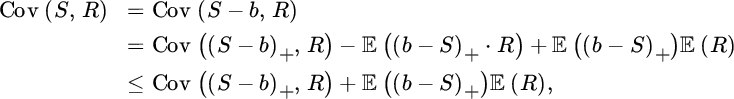
with equality if R(S) = 0 whenever 0 ≤ S ≤ b. Using this bound in (8.2.12), and applying the Cauchy–Schwartz inequality for the resulting covariance, we get

(8.2.13)

If we now postulate

(8.2.14)

for a sufficiently regular function f, then R only appears through its variance in the above inequality and with

(8.2.15)

it can be reexpressed as

(8.2.16)

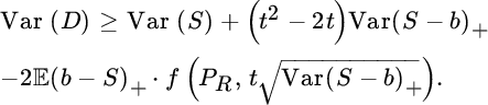
At the same time, we see from the Cauchy–Schwartz inequality that equality is achieved in (8.2.16) when

(8.2.17)

for some positive constant a, which from the requirement R(S) ≤ S is also bounded by 1. Hence we have identified the optimal reinsurance form and it only remains to determine the constants 0 < a ≤ 1 and b ≥ 0, which we get by minimizing the right‐hand side of (8.2.16) w.r.t. t. Under weak conditions on f (which are fulfilled for our cases of interest here), one can show that the right‐hand side is convex in t attaining a minimal value, which then by (8.2.15) has to be equal to a.

We hence obtained that whenever P_R is fixed and the premium principle can be described by (8.2.14), then a change‐loss contract (8.2.17) minimizes the retained variance, where the optimal constants a and b are determined by the two equations

and

(8.2.18)

Let us consider three examples:

• For the expected value principle we have f(P_R, t) = P_R/(1 + θ) and we obtain R(S) = (S − b)₊ with , which brings us back to Section 8.2.3.1 (cf. (8.2.10)).
• For the standard deviation principle we have f(P_R, t) = P_R − α_S t, and (8.2.18) simplifies to .
• Finally, for the variance principle the function is f(P_R, t) = P_R − α_V t², and (8.2.18) simplifies to .

The rigorous proof of the above result can be found in Kaluszka [478], where also an adaptation for identifying the optimal XL treaty under minimizing the aggregate retained variance is given (which is again of change‐loss type) and further premium principles satisfying (8.2.14) are discussed (for the standard deviation principle (see also Gajek and Zagrodny [364])).

If, in addition to the above problem formulation, we ask for a prespecified target value (and hence also is fixed), then in (8.2.13) the expression for can be replaced by that fixed quantity directly, and when now implementing the substitution (8.2.15), the last term in (8.2.16) does not depend on t. Correspondingly, the right‐hand side is minimized either by t = 1 or the largest possible t value that still is in line with the constraint (if that value is smaller than 1). Correspondingly, the optimal reinsurance form minimizing Var (D) then is

and hence again of change‐loss type, where the constant b depends on the distribution of S and is determined by a suitably adapted equation (see Kaluszka [480] for details).

There are many variants of these types of results (see the Notes at the end of the chapter for more information).

8.2.4 Maximizing Expected Utility

In a number of cases the utility framework of Section 8.2.1 is considered for one party marginally, and in particular one may ask for the reinsurance treaty that maximizes the expected utility of the cedent, that is,

(8.2.19)

where u denotes the utility function of the cedent, and w his current wealth (here considered a deterministic number which includes already the received premiums from the policyholders). The concrete optimal solution will now depend on the imposed conditions (e.g., the premium rule P_R and the class of admissible reinsurance forms R under consideration).

For instance, if the cedent has a risk‐averse (i.e., concave and increasing) utility function u(x), and if the reinsurance premium P_R is fixed, then the function v(x) = −u(w − P_R − x) is increasing and convex. As a consequence, in (8.2.19) we in fact look for D = S − R that is minimal in terms of stop‐loss order. If the reinsurance premium is calculated according to the expected value principle, the argument of Section 8.2.3.1 in terms of the ≺ _da‐order applies in the same way, again identifying the SL contract as optimal. The optimality of a SL treaty in the context of risk‐averse utility functions was already established by Arrow [46] (see also Borch [150]). If in addition there is an upper limit on the reinsurance coverage, then a SL contract with that upper limit is optimal (cf. Cummins and Mahul [241]). For an adaptation of Arrow’s result when the reinsurer imposes an upper limit of its expected loss, see Zhou and Wu [808].

As another example, consider a cedent facing total risk S and receiving an offer P_S as reinsurance premium for the entire risk S. On that basis the cedent now decides about the extent (fraction a) to which he wants to enter this treaty (assuming that the reinsurance premium scales according to the proportionality factor a of the resulting QS treaty). Then (8.2.19) turns into

For exponential utility u(x) = −e^−αx and normally distributed risk , this leads to a remarkably simple expression for the optimal retained fraction:

It is proportional to the safety loading of the reinsurance premium offer, and inversely proportional both to the risk aversion coefficient and the variance of the risk S. Even if for QS treaties the pricing often works slightly differently (cf. Section 7.3), this formula is of particular interest, as it has a striking resemblance to the Merton ratio in optimal portfolio theory (although there S is log‐normally distributed and u is a power function) (cf. Gerber and Pafumi [387]).

Deprez and Gerber [279] consider (8.2.19) for convex, Gâteaux‐differentiable premium rules P_R = H(R), and show for any risk‐averse utility function u by a simple perturbation argument that the general solution of this maximization problem then is the reinsurance form R^* that satisfies

(8.2.20)

(the argument in fact also applies when w is replaced by a random initial position W that is independent of S). Note that the random variable H^′(R) is a gradient for which

for any random variable V and hence measures the sensitivity of the premium for small changes of the underlying risk.

Particular principles of premium calculation for which the above result applies are the pure premium principle with H^′(R) = 1, the variance principle (7.1.3) with , the standard deviation principle (7.1.4) with Gâteaux derivative and the exponential principle (7.1.5) with . For example, if the utility function of the insurer is exponential with risk aversion b and the premium principle of the reinsurer is (7.1.5) with risk aversion a, then (8.2.20) turns into

which specifies R^* up to an additive constant. Choosing the latter in such a way that R^*(0) = 0, we then get

that is, a QS contract where the proportion is determined by the risk aversion of the insurer and reinsurer. Note that this exactly corresponds to the risk‐sharing agreement of the example in Section 8.2.1, as both the insurer and reinsurer here essentially make decisions based on exponential utility.

Finally note that if the reinsurer offers a pure premium principle , then by (8.2.20) R^* − S must be a constant, for example leading to R^*(S) = S. That is, with risk averse utility, the insurer should exploit the “cheap” premium offer of the reinsurer to the largest possible extent.

8.2.5 Minimizing the Ruin Probability

8.2.5.1 One‐year Time Horizon View

Let us first stick to the discrete setting of the previous sections and look for the reinsurance form that minimizes the ruin probability at that future time point (say, one year from now), that is,

(8.2.21)

Clearly, if this is the criterion and we can afford full protection, then a SL contract will lead to a ruin probability equal to 0. If for a premium P_R we can purchase the cover R = (S−(w − P_R))₊, then this is optimal. However, there are two issues to note here. First, in many situations this will not be feasible, that is, one may only be able to afford a SL contract R = (S − b)₊ with w − P_R < b, and in that case the cover does not help at all to improve the survival probability. And secondly, if such a cover costs already more than the earned premium P on the original policies and if one’s goal is to minimize ruin, then it is preferable to stay out of those policies altogether, as one then stays positive (with the capital w − P available before writing policies) with probability 1 (one may indeed question in general the suitability of the criterion of minimizing ruin from this perspective).

Let us still take the viewpoint that the first‐line business is already written (with the collected premium being already contained in w) and the goal is to minimize the remaining ruin probability. Assume also that the reinsurer offers protection according to an expected value principle, that the reinsurance premium amount P_R is fixed and the above full protection can not be afforded (note that Arrow’s result on the optimality of an SL treaty does not apply here, since the indicator function on the right‐hand side of (8.2.21), interpreted as a utility, is not concave). Gajek and Zagrodny [366] showed that then, if S is a continuous random variable, the best possible contract is of the form

(8.2.22)

where c^* is the largest value that can be afforded for this contract with the amount P_R, that is, a truncated SL contract minimizes the ruin probability. The result is somewhat intuitive, as one tries to get full protection for an as large claim size as possible (for empirical evidence and a discussion of the popularity of such treaties in catastrophe reinsurance, see Froot [360]). The proof is based on an application of the Neyman–Pearson lemma (cf. [366] for details. See also Bernard and Tian [127]).

8.2.5.2 Infinite‐time Ruin Probability

Let us continue the viewpoint that first‐line business is already written and the insurer wants to identify for a given premium rule of the reinsurer the reinsurance strategy that minimizes the probability of getting ruined. However, now consider the long‐term view of the probability of never getting ruined (the infinite‐time ruin probability). The underlying risk model can be in discrete time (aggregate claims and premiums are checked at the end of each time period, say a year) or in continuous time when the monitoring is done continuously. The idea is to fix a reinsurance strategy in the beginning that is then kept through time. As argued in Chapter 7, the underlying philosophy is not to indeed follow that same strategy forever, but to get a feeling of the effects of such a strategy on the safety in the long run. Note again that the problem is only non‐trivial, when one assumes that reinsurance premiums are higher than first‐line premiums (otherwise the entire portfolio could be passed on to the reinsurer, leading to zero ruin probability).

The Lundberg bound (7.2.13) was shown to hold for a continuous‐time model with adjustment coefficient defined in (7.2.12). For a risk model in discrete time, (7.2.13) also holds, where the adjustment coefficient is then the positive solution γ of

with P the premium income and S the aggregate claim per time unit (e.g., see [57]).

The bound (7.2.13) turns out to be a quite good approximation for the true value of the ruin probability ψ(w) in many cases and due to its simplicity it is often used as a (conservative) approximation ψ(w) ≈ e^−γw. Then, for both continuous‐ and discrete‐time models the problem of minimizing the ruin probability is translated into maximizing the adjustment coefficient.

In a number of situations, maximizing the adjustment coefficient can be translated back to minimizing convex order. For instance, consider the Cramér–Lundberg process and its adjustment equation (7.2.12). Then one sees immediately that by the convexity of the function v(x) = e^rx, the retained risk that maximizes γ in (7.2.12) is the one that is minimal with respect to convex order (under the assumption that the reinsurance premium is calculated according to an expected value principle with fixed loading, which leaves the left‐hand side of (7.2.12) invariant for all considered forms D). By the arguments of Section 8.2.3.1 the latter brings us to the result that an XL treaty maximizes γ (as the optimality of the SL treaty translates into XL, when only individual treaties are considered) (e.g., see Gerber [383]). Centeno [189] gives an algorithm to calculate the optimal retention for this XL treaty. The result by Gerber is extended by Hesselager [440] in the sense that, if the insurer can freely choose among global and individual reinsurance contracts with the same pure premium and reinsurance loading, then the adjustment coefficient will be maximized by a SL treaty. Waters [775] investigates the dependence of the adjustment coefficient on the retention. He does this for proportional, SL and XL reinsurance contracts and under a variety of different premium schemes (see also Hald and Schmidli [418]).

In [188], Centeno considers change‐loss contracts on individual claims, that is,

and for a compound Poisson model studies the combination of parameters a and M that maximizes the adjustment coefficient for the first‐line insurer, also when a target value on the expected income is fixed.

An intimate connection between maximization of the adjustment coefficient and maximizing expected utility for an exponential utility function is exploited in Guerra and Centeno [413, 414], who establish optimal reinsurance treaties when the premium principle of the reinsurer is a convex functional. It turns out that for an expected value principle, the optimal form is of SL type, whereas for variance and standard deviation principles the optimal R(S) is a non‐linear function of S, which is not among the reinsurance forms typically employed in practice. For strategies restricted to the individual claim level, see [194].

For heavy‐tailed claims, the adjustment coefficient does not exist, but with an unlimited XL cover the maximum retained claim size is upper‐bounded by the retention, so that then γ exists again for the first‐line insurer and the above approach to maximize γ still makes sense. One should keep in mind, however, that maximizing γ is only an approximate solution for minimizing the ruin probability ψ(w). Under certain model assumptions one can go in fact much further. In the following, we give an illustration.

Consider the Cramér–Lundberg model and compare any two c.d.f. F₁ and F₂ for the claim size through convex ordering.From the Pollaczeck–Khintchine formula (7.2.10), which gives an exact expression for ψ(w) for any claim size distribution, one then sees that F₁ ≺ _cxF₂ implies ψ₁(w) ≤ ψ₂(w), since convex order is preserved under convolution and compounding (e.g., see [57, Prop. IV.8.2] for details). As for previous instances, this result can then be used to show in a simple way that if the reinsurance premium is calculated with an expected value principle, an unlimited XL treaty minimizes the ruin probability among all reinsurance forms applied to individual claims. Indeed, compare any reinsurance form candidate D = X − R with an XL treaty, the retention M of which is chosen in such a way that (i.e., the two treaties have the same premium). Denote by F_D the c.d.f. of D(X) and by F_XL the c.d.f. of min(X, M). Indeed, by the same arguments as in Section 8.2.3.1, one gets F_XL ≺ _daF_D and by the identical mean subsequently F_XL ≺ _cxF_D, so that

for all capital values w.

With the same technique one can also show that if the reinsurer poses the additional constraint that R(X) ≤ L, then an L xs M treaty is optimal. Indeed, consider again any alternative D = X − R for a premium P_R and choose M such that , so that the two reinsurance premiums coincide. Let F_D and F_XL again denote the c.d.f. of the retained claim. Then F_XL ≺ _daF_D, because for x < M, F_XL(x) = F_X(x) ≤ F_D(x) as above, whereas for x ≥ M one has F_XL(x) = F_X(x + L). However, the limit X − D ≤ L leads to D ≥ X − L, that is, F_D(x) ≤ F_X(x + L) (even for all x). Consequently, F_XL ≺ _slF_D and since the retained amounts have the same mean, further F_XL ≺ _cxF_D. However, the latter again implies that for all w ≥ 0

that is, an XL treaty with layer L minimizes the ruin probability ψ(w). This result holds for any claim size distribution (which is relevant to note, as due to the finite layer L a heavy‐tailed claim stays here also heavy tailed after reinsurance, so the adjustment coefficient does not exist at all).

Section 8.7 will discuss dynamic reinsurance strategies for continuous‐time risk models.

8.2.6 Combining Reinsurance Treaties over Subportfolios

The first insurer often needs to deal with many (sub)portfolios simultaneously. It is then natural to look for an optimal combination of reinsurance forms to achieve an overall objective. In this section we will consider two classical approaches (one on a combination of proportional treaties and one on the non‐proportional case) that originally go back to de Finetti [255].

Assume that the insurer has to deal with I subportfolios with total claim amounts {S_i, 1 ≤ i ≤ I} that will be divided into deductible and reinsured amounts by S_i = R_i + D_i, 1 ≤ i ≤ I.For simplicity we assume that the portfolios are independent and that the type of reinsurance is the same for all of them. If the premium received for covering S_i is P_i and the reinsurance premium is , then the total income amounts to

The following results are obtained now under the objective to maximize , given a constraint on Var (U).

8.2.6.1 Proportional Reinsurance

If we look for the best combination of QS treaties across the subportfolios, then R_i = a_iS_i. For the premium principle of the reinsurer consider an expected value principle

(8.2.23)

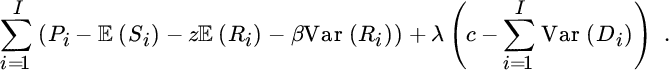
for (possibly different) positive constants z_i, 1 ≤ i ≤ I. Maximizing under the condition Var (U) = c for a fixed constant c can now be done by the method of Lagrange multipliers. Let λ be such a multiplier. We need to maximize the expression

by choosing the proportions a_i, 1 ≤ i ≤ I properly. The expression becomes

Equating the partial derivative with respect to a_i with zero leads to

so that

(8.2.24)

where the constant λ is determined by the side condition on the variance. Concretely, if a_i > 0 for all i = 1, …, I, then

Note that the retained proportion 1 − a_i depends in a crucial way on the value of the dispersion of S_i (the greater the dispersion of S_i, the smaller the retained proportion 1 − a_i). Also, the retained proportion is higher if reinsurance is more expensive.

This result has an interesting consequence: interpret each risk X_i in a portfolio as a subportfolio on its own (containing only one risk). In that case, of course the claim history will not be sufficient to estimate the first two moments of each such claim size. However, as discussed in Section 7.4.1.2, for certain lines of business (like property lines) it is reasonable to assume that the loss degree V with respect to the sum insured (or PML) Q_i is identically distributed (here it is in fact sufficient that the first two moments coincide), i.e. and Var (V) = σ², 1 ≤ i ≤ I. It is also reasonable to assume that all safety loadings z_i are equal, and then (8.2.24) simplifies to

That is, the resulting proportionality factors are a constant divided by Q_i (and a_i = 0 if Q_i < M), but this is the structure of a surplus reinsurance contract! Hence the present setting suggests a situation and criterion within QS strategies for which a surplus treaty is optimal, and one may in fact use the above reasoning as a guideline for the choice of the retention M. For an extension of this result to include cost‐of‐capital considerations, refer to Section 8.3.

If the reinsurance premium principle (8.2.23) is extended to include a variance component

(8.2.25)

for some β > 0, then a similar calculation yields the adaptation

so the variance term in the premium principle adds a fixed proportion for all subportfolios.

8.2.6.2 Excess‐of‐loss Reinsurance

Let us now look for the best choice of retention a_i of an XL treaty for subportfolio i with total risk S_i, which is assumed compound Poisson distributed with rate λ_i and claim sizes and c.d.f. F_i (in contrast to above, here the result will not only depend on the first two moments, but on the entire distribution). The deducted part of subportfolio i then is

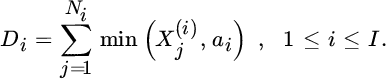
Let us consider a reinsurance premium principle of the general form (8.2.25). Then under the same variance condition as above we have to maximize the expression

By the Poisson assumption we see that for 1 ≤ i ≤ I (cf. also Section 2.3.1),

The equation for a_i is therefore given by

This leads quickly to the solution

(8.2.26)

where λ is determined by the condition

Equation (8.2.26) can be rewritten as

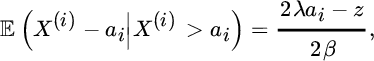
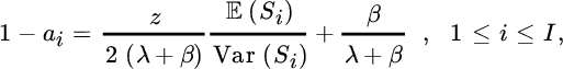
which is an equation for a_i in terms of the mean excess function of the individual claim sizes. The existence and the value of the solution depend heavily on the form of this mean excess function. The right‐hand side is a straight line in the variable a_i, starting at the value − z/(2β) and increasing with slope λ/β. The function on the left starts at the positive value but behaves differently depending on the tail behavior of the distribution. If the tail is exponentially bounded, then a unique solution exists. If, however, the distribution is strict Pareto with index α, then a solution only exists if α > 1 + β/λ.

It is interesting to see that an increase in results in a similar increase of the retention a_i. Also note that in the absence of a variance component in the premium principle (8.2.25), that is, β = 0, it follows from (8.2.26) that there is a constant retention a_i = z/(2λ) across the subportfolios. Indeed, in practice it seems rather common not to vary the retention of XL treaties across different subportfolios.

8.3 Solvency Constraints and Cost of Capital

In Section 7.2.2 we discussed how the safety loading in insurance premiums may be determined in order to meet capital costs arising from regulatory solvency constraints. At the same time, for the final first‐line insurance premium P(1) further factors will play a role, (prominently) including market competition. Let us therefore now assume that the premium P = P(1) is already given and fixed, and we look for reinsurance to improve the overall situation.

Recall that the solvency capital requirement for the annual loss is determined by some risk measure ρ (typically VaR or CTE). In addition to the viewpoint of Section 7.2.2, let us now assume that the capital costs increase the annual loss (e.g., because they are paid to external investors). Then, instead of S − P, the annual loss is

and the final necessary solvency capital will be higher than ρ(S − P), leading to the recursive relationship

which yields

(we use here that ρ is positively homogeneous and translation‐invariant, cf. Section 7.1). The resulting gain (i.e., negative loss) at the end of the year (without reinsurance) then is

(8.3.27)

If a reinsurance treaty is entered for a premium P_R, this changes to

(8.3.28)

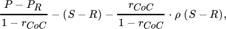
and one can now again try to find optimal reinsurance forms R according to the criteria discussed in the previous sections, now with the correction factor for cost of capital (and hence the solvency constraint) included.

For instance, if P is fixed and the goal is to maximize the expected income after reinsurance, one obtains from (8.3.28) that the goal is to identify R for which

(8.3.29)

is attained. This approach of looking at the capital cost problem can be found, for example, in Kull [514], who gives a variety of optimal reinsurance results under this setup. For an expected utility approach of (8.3.28) in the spirit of (8.2.4), see Haas [417].

It may also frequently happen that the amount of available risk capital is fixed (a risk budget is available), and then one has to identify the reinsurance form that maximizes some objective (e.g., expected profit) given this capital constraint. Also, sometimes the overall risk capital of a company is fixed (by some general considerations) and then the question is how to most efficiently allocate this capital to subportfolios, that is, to design reinsurance arrangements on the individual subportfolios whose risk capital implications aggregate to the overall target. In this context, an extension of the problem of optimal proportions of subportfolios of Section 8.2.6.1 to the case with capital costs was developed by Kull [514]. Capital and its allocation have recently become crucial in the light of risk‐based management of insurance companies, so the criteria discussed in the present section can be regarded as particularly relevant for applications (cf. Dacorogna [243]).

A variant of the above criterion is to focus on the expected profit relative to the required solvency capital. The goal then is to maximize the return on risk‐adjusted capital (RORAC), which in the notation of Section 7.2.2 translates into

(8.3.30)

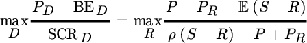
for given first‐line premium P, aggregate claim size S, reinsurance premium rule P_R and risk measure ρ. That is, here r_CoC is not prespecified, but the quantity to be maximized. One immediately sees that under this criterion a QS treaty R = aS with P_R = aP is not of interest at all, as it does not change the ratio (only P_R < aP would be of interest).

Lampaert and Walhin [526] use the RORAC criterion (8.3.30) to compare quota share and surplus treaties with both fixed and variable proportions (lines, respectively). Performing an empirical study on a large data set from reinsurance practice, they conclude under some additional assumptions (including expected value premium principles for both P and P_R, with fixed safety loading for all risk sizes) that it is not beneficial to use tables of lines constructed by an inverse rate method (cf. Section 2.2), which is contrary to what one may intuitively expect. It is, however, beneficial for the RORAC criterion to construct a table of lines according to the method of Section 8.2.6.1.

It will be useful finally to adapt the obtained results to include claims reserves, market risk, counterparty risk etc. in the calculation of the solvency capital requirement and respective cost of capital. However, the resulting optimization problems then quickly become complex, and their solutions heavily depend on the respective posed assumptions.

8.4 Minimizing Other Risk Measures

In recent years many variants of the optimization problem

(8.4.31)

have been studied in the literature. For instance, Cai and Tan [178] studied the subproblem of optimizing retention levels within SL contracts for (8.4.31) when ρ is the VaR or CTE and P_R is determined by an expected value principle. Cai et al. [179] then extended this analysis to a larger class of contracts, indicating that change‐loss contracts (and QS and SL as special cases) are optimal. For a comparison across reinsurance premium principles, see Tan et al. [727]. An extension to optimal treaties in the presence of several reinsurers can be found in Asimit et al. [52].

Balbas et al. [73] provide an in‐depth study on characterizing optimal reinsurance forms under (8.4.31) for a general class of risk measures ρ by exploiting duality theory in functional analysis. It is shown that a SL treaty is often optimal when P_R is an expected value principle. For investigations on the stability of optimality results when switching from one risk measure to another, see Balbás et al. [74]. Also, Balbás et al. [72] identified optimal reinsurance forms when there is uncertainty about the involved claim distribution (see also Asimit et al. [53] and Bernard et al. [123]).

Another risk measure that has recently gained considerable attention due to discussions on backtesting issues for risk measures is the expectile, see, for example, Ziegel [811], Bellini et al. [107], and Bellini and Bignozzi [106]. Cai and Weng [175] show that for certain reinsurance premium rules a superposition of two limited XL treaties is then optimal, where the reinsurer takes over two disjoint layers.

The criterion (8.4.31) is not likely to directly be a driving criterion in practice, as then (akin to minimizing the ruin probability in Section 8.2.5) it is optimal to stay out of the insurance business altogether, resulting in a zero value for ρ. However, if one takes the viewpoint that the primary business is already written and reinsurance premiums are more expensive than premiums in primary markets, then the identification of reinsurance forms minimizing such risk measures leads to interesting mathematical problems. Moreover, minor modifications can embed the solutions into the cost‐of‐capital framework of Section 8.3. To see this, note that by translation‐invariance of ρ, the optimization problem (8.3.29) can be rewritten as

(8.4.32)

and so the goal of maximizing the expected gain under regulatory solvency constraints translates into minimizing the risk measure ρ of a weighted sum of the safety loading in the reinsurance premium, the retained risk S − R and . If, for instance, , then (8.4.32) simplifies to the problem

so that results for (8.4.31) can be interpreted within the framework of (8.4.32) for a modified value of θ_R.

For optimal risk‐sharing rules for convex risk measures expressed in the framework of monetary utility functions, see Jouini et al. [471], Barrieu and El Karoui [85], as well as Acciaio [7], who studied optimal risk sharing under non‐monotone risk measures. A general solution to this problem is provided by Filipović and Svindland [351], who showed that for law‐invariant convex risk measures on the model space L^p, where , the optimal risk allocation always exists and is composed of increasing Lipschitz continuous functions of the aggregate risk. For a study based on spectral risk measures, see Brandtner and Kürsten [160]. Barrieu and Scandolo [87] extend the Pareto‐optimal allocation analysis to a multi‐period situation by dealing with preference functionals on general vector spaces.

8.5 Combining Reinsurance Treaties

We have seen above that in some cases a change‐loss contract turns out to be optimal, where a SL (or XL) feature is put on top of a QS arrangement. Apart from defining a contract with such a structure, the first‐line insurer can also apply different reinsurance treaties simultaneously, which together lead to (or approximate) the desired coverage structure. For instance, a reinsurer may offer only a certain lower layer in an XL treaty, and another reinsurer specializing in catastrophe reinsurance may offer a treaty for a higher layer. Sometimes also the premium offer from a reinsurer may only be attractive for a certain part of the coverage, and a combination of two separate treaties is then preferable. Such combinations are frequently applied in reinsurance practice. Naturally, however, it is difficult (if not impossible) to formalize such a demand/supply situation together with the premium rules and objectives in order to identify a certain combination as optimal. One may rather be restricted to choosing an optimal parameter of an already pre‐specified reinsurance form. For a study of this kind, see Verlaak [759] and Verlaak and Beirlant [760], where a variety of different combinations are tried out under a mean‐variance optimality condition. We list here a few further examples:

• Suppose that there are n independent portfolios and that the claims in the ith portfolio are given by {X_{i, j}, 1 ≤ j ≤ N_i}. A QS treaty with factor a_i is applied to this portfolio together with an XL treaty with retention M_i. The overall retained risk for the first‐line insurer then is
  
  In Centeno and Simões [195], the determination of the factors a_i, (1 ≤ i ≤ n) and the retentions M_i, (1 ≤ i ≤ n) under a minimization of the adjustment coefficient is treated (for an early reference, see also [187]).
• For a combination of surplus and XL treaties, see Benktander and Ohlin [114].
• Combinations of proportional and SL contracts are treated by, for example, Schmitter [679]. As another form to combine these two reinsurance forms, Hürlimann [453] uses a mixture qX + (1 − q)(X − C)₊. Under some reasonable optimization criteria, one of the two reinsurance types prevails.

8.6 Reinsurance Chains

Another way of introducing more than one insurer is to deal with the risk in a hierarchical cascade (retrocession). Let the original risk be denoted by X. The first company faces the risk X, gets a premium P₁ and buys reinsurance for a part X₂ from a first reinsurer for a premium P₂. This company itself accepts X₂ as its own risk but in turn takes reinsurance for a part X₃ for a premium P₃. Ultimately, the nth reinsurer keeps the remaining part X_n. If one studies the question of optimal sharing in a utility framework, then the ith partner with utility function u_i will try to maximize

where X₁ = X and P_n+1 = 0. Note that the Pareto‐optimal risk sharing discussed in Section 8.2.1 has a similar flavor, but here the sequential character of the decision process leads to different results. For an early contribution on this problem for proportional treaties, certain choices for utility functions and premium rules, see Gerber [384]. Substantial generalizations of this problem have been investigated in d’ Ursel et al. [312], Lemaire et al. [537], and Heijnen et al. [430, 432].

A critical question in the distribution of reinsurance is the optimal number of reinsurers and their respective responsibilities (e.g., see Powers et al. [626]). It also needs to be ensured that through repackaging of risks, retrocession does not lead to a cycle. One unfortunate such case in history is the so‐called LMX spiral in the early 1990s (see Baluch et al. [76]).

8.7 Dynamic Reinsurance

In Section 8.2.5.2 we discussed the criterion of minimizing the ruin probability for a discrete‐time or continuous‐time surplus process through an optimal form of reinsurance. There the assumption was that the concrete form of the reinsurance treaty has to be chosen in the beginning, and then does not change over time. In the academic literature it has also been studied by how much the overall target (of minimal ruin probability) could be improved if one were allowed to adapt the reinsurance form along the way. When the surplus process is of Markovian type, the optimal strategy is typically a feedback strategy, which for the ruin probability criterion at each time point only depends on the current value of the surplus process.

For a discrete‐time risk process, the respective optimal adaptation at each time point can be obtained by stochastic dynamic programming. In most cases one cannot obtain explicit results, but approximate the optimal solution numerically (see Schäl [669] for a theoretically sound basis of respective numerical algorithms). In the setting of classical continuous‐time risk models (like the compound Poisson model), from a mathematical point of view somewhat more explicit results can be obtained if the times at which one can adapt the reinsurance form are not fixed (e.g., annual) time points, but are the claim occurrence times, as then the underlying process is a random walk with much simpler increment distribution. However, this little advantage comes at the expense of a less realistic model setup, as adapting the contract at every single claim occurrence will not be feasible in applications.

If, instead, one switches to the possibility of continuous‐time adaptation of the contract, the analysis becomes more transparent. Mathematically, the minimal ruin probability (value function) can then often be determined by solving a Hamilton–Jacobi–Bellman (HJB) equation and in a number of cases also the corresponding optimal dynamic reinsurance strategy can be identified. It should be noted that an actual implementation of such a continuous‐time adaptive strategy is even less “realistic”, but this approach allows the potential improvement through continuous‐time action (compared to a static strategy) to be quantified, and also gives some intuition for the suitability (and long‐term consequences) of parameter choices within certain types of contracts.

When trying to solve such a stochastic control problem, a number of challenges arise. The solution of the HJB equation usually can only be obtained numerically and is just a possible candidate for the value function, and a separate verification step is needed. Also, the solution of the HJB equation may not be unique, and the value function may not be as regular as is needed for the equation. Correspondingly the actual calculations can be highly involved, and it is beyond the scope of this book to provide details on these aspects (see Schmidli [676] and Azcue and Muler [70] for profound surveys on all the mathematical aspects in such an approach). Instead, for illustration we simply state here the results one obtains for the classical risk model.

Consider the Cramér–Lundberg model (7.2.8) with a dynamic reinsurance strategy u_t = u_t(X_i), where u_t(X_i) is the retained amount of claim X_i for the cedent when the claim occurs at time t. Let c_R(u_t) be the reinsurance premium intensity for strategy u_t and assume that more reinsurance is more expensive as well as c_R(0) > c (otherwise it would be optimal to reinsure the entire portfolio, see also Section 8.2.5). Then the optimal control problem is to identify u_t such that the ruin probability for the process

is minimized, where T_i is the occurrence time of the ith claim.

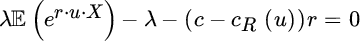
• Dynamic proportional reinsurance: u(y) = u y with 0 ≤ u ≤ 1 If one can dynamically adapt the proportionality constant in a QS contract, then (under the weak condition ) it turns out to be optimal for the cedent not to purchase any proportional reinsurance as long as the current surplus is below a threshold value w₀ (i.e., u = 1 for any w < w₀). This may at first sight not look intuitive, as particularly for small surplus values reinsurance can be useful, but since reinsurance is expensive, for the long‐term goal of minimal ruin probability it is then preferable to not pay reinsurance premiums and use the premium income from primary insurance to more quickly decrease the ruin probability before one can “afford” reinsurance again. Furthermore, if a solution γ_R > 0 to the equation
  (8.7.33)

  exists, then (under mild assumptions) the asymptotic behavior of the ruin probability improves (from the Cramér–Lundberg approximation (7.2.14) without reinsurance) to

  (8.7.34)

  for some constant C > 0. If the optimal value u^* for which the infimum in (8.7.33) is attained is moreover unique, then , that is, the optimal proportionality factor converges to a constant for increasing surplus.

  Note that due to the continuity and convexity properties of the involved functions, γ_R defined through (8.7.33) is also the supremum across all fixed u of the maximal solution of . Hence the adjustment coefficient obtained by optimal dynamic proportional reinsurance is the same as the one obtained from determining the static u for a QS treaty that maximizes the adjustment coefficient (cf. Section 8.2.5.2). Correspondingly, dynamic reinsurance cannot improve the optimal adjustment coefficient among static QS treaties. However, for moderately sized surplus values, dynamic reinsurance can of course outperform the best static counterpart.

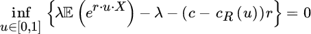
• Dynamic XL reinsurance: If it is possible to dynamically adapt the retention level u, then for exponentially bounded claims one can show (under some mild additional conditions) that also here an asymptotic behavior of the form (8.7.34) holds, if a solution γ_R > 0 to
  

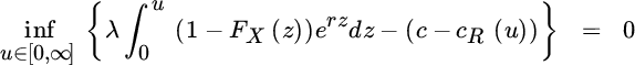
  exists. If the minimizer u^* is unique, then , that is, the optimal retention again converges to a constant value for increasing surplus. As for the proportional case, the resulting adjustment coefficient of the best static strategy cannot be improved through dynamic adaptation.

Several variants of the stochastic control problems of the above type have been studied extensively in the literature, in particular also in connection with optimal investment of parts of the surplus in the financial market and optimal dividend payments (see the Notes at the end of the chapter).

8.8 Beyond Piecewise Linear Contracts

One observes that almost all contracts identified as optimal in this chapter exhibit a piecewise linear shape of R(X) (or R(S)) and likewise the corresponding retained amount. This is nicely in line with the fact that most of the reinsurance forms implemented in practice are of such a form. However, the question arises whether there could not exist more efficient ways for risk sharing, particularly since one may be inclined to think that smoother transitions between two regions are preferable to non‐differentiable kinks (at junction points of linear pieces, like at the retention). This line of reasoning of course hinges on the underlying objectives and constraints for the optimization procedure. When using first and second moments of the retained risk as criteria, then piecewise linear solutions are no surprise. Note that for some other criteria in this chapter, such as in Sections 8.2.5 and 8.4, one sometimes also received optimal shapes of piecewise linear form because – in loose terms – on from a certain point (determined by some constraint) maximal coverage was needed until the available reinsurance premium is used up. It is natural to expect that in more general models or under different criteria non‐linear shapes will be optimal. Among the cases for which this was already explicitly studied and shown, are:

• in the presence of default risk of the reinsurer (e.g., see Bernard and Ludkovki [125])
• in some cases when maximizing a linear combination of insurer’s and reinsurer’s utility (e.g., see Albrecher and Haas [20])
• taking into account cost‐of‐capital considerations (cf. Section 8.3)
• maximizing the adjustment coefficient under a variance principle or standard deviation principle for the reinsurance premium (cf. Section 8.2.5.2).

Even if non‐linear retention functions are clearly non‐standard in practice in an explicit form, they do appear implicitly as a result of certain combinations of reinsurance contracts and profit‐sharing mechanisms.

Using non‐linear shapes is also quite conceivable from a general viewpoint: reinsurance is about reshaping the insurer’s loss distribution (often referred to as tapering in engineering circles), and if one has a target distribution for the retained amount, then one can define a respective retention function that leads to the desired target. For instance, if the goal after reinsurance of X is an exponential distribution with parameter λ for D, then

(8.8.35)

serves the purpose, since

and F_X(X) is uniformly distributed on [0, 1]. Note that (8.8.35) ensures 0 ≤ D(X) ≤ X as long as we have F_X(x) ≤ 1 − e^−λx for x ≥ 0 (which, for large x, is the case of interest). For instance, if X is a strict Pareto random variable with F_X(x) = 1 − (x/x₀)^−α, x ≥ x₀ > 0, then

has the desired exponential distribution. Intuitively, rather than accepting the entire tail of X like in unlimited XL, the reinsurer accepts a larger proportion of the claim, the larger its size is. In a practical implementation, both the XL contract and such a contract (8.8.35) would only be written with an upper limit, but the latter can result in a considerably cheaper reinsurance form for the cedent than passing on an entire layer. Depending on the employed objectives and constraints, this may also be the formal solution of an optimization problem, in particular when involving capital costs in the criteria.

Finally, we mention another non‐standard reinsurance form that is not implemented, but which could have nice properties in terms of reshaping the tail. In a randomized reinsurance contract, the reinsured amount R(X) is not a deterministic function of X, but the mapping R is a random variable itself, that is, once X is known, there is an additional random mechanism to determine the reinsured amount according to some given distribution (e.g., a lottery under the supervision of a notary). While there may be several practical (and psychological) arguments against such a type of treaty, it can serve as an interesting thought experiment, since randomization is another effective tool for reshaping a loss distribution (in a possibly cost‐effective way) (see Albrecher and Cani [17]). For the criteria of Section 8.2.5.1, Gajek and Zagrodny [366] showed that for certain discrete loss variables, a randomized reinsurance form in fact outperforms the deterministic ones.

A final general comment is in order. Even if one is able to formalize the objectives and constraints, and identify a corresponding optimal reinsurance form, in practice this particular contract may not be available or negotiable. In that case, one will look at all available reinsurance forms, determine the parameters (like the retention) such as to match the safety criterion and then choose the cheapest among those. In fact, some of the approaches discussed above dealt with identifying the best parameters within a given reinsurance form. It should be mentioned, however, that in such a procedure one should also be careful with model risk and estimation risk. At the same time, from the viewpoint of capital costs, whenever the resulting reduction of capital costs exceeds the reinsurance premium, the reinsurance contract will be of interest, even if the underlying model may have a certain degree of inaccuracy.

8.9 Notes and Bibliography

The modern economic theory of efficient risk sharing can be traced back to Borch [148, 151, 152] and Wilson [791]. Later, Arrow [47, 48] and in a more general framework Raviv [641] showed that the safety loading in insurance contracts leads to optimal insurance contracts containing deductibles. For an overview, see also Eeckhoudt et al. [313]. Gerber [385] extends Borch’s equilibrium theorem (see also Pressacco [630] and Taylor [732, 733]). An alternative approach to Borch’s result based on comonotonicity is Cheung et al. [206] and an extension to the more general notion of essential margins is Flåm [355]. Criterion (8.2.1) is also known as the weighted‐sum or scalarization method in multi‐objective optimization (cf. Ehrgott [314]). Note that the constants k_i in (8.2.1) can alternatively be interpreted as Lagrange multipliers of a marginal expected utility problem formulation with lower bounds on the expected utilities of the other companies. Knispel et al. [494] look into the effects of enlarging the number of (re)insurers and the implied diversification with respect to Pareto‐optimal allocations. Recently, Malamud et al. [560] extended the results of Raviv to the situation where n reinsurers are available and the optimal reinsurance contracts R₁(S), …, R_n(S) with are determined in an expected utility framework with given risk‐averse utility functions for all participants, leading to different deductibles and proportionality constants for each reinsurance contract. A related study of the role of the leading reinsurer is Boonen et al. [147]. For a nice recent survey on optimal reinsurance from an economical point of view, refer to Bernard [120].

Cummins et al. [240] use the proportionality result of Section 8.2.1 to assess the capacity of the (re)insurance market for catastrophic losses in view of limited liabilities. Ludkovksi and Rüschendorf [550] provide deeper insight into the comonotonicity property of Pareto‐optimal risk allocations. An attempt to bridge the actuarial and economic view of reinsurance is Aase [2], who gives an economic equilibrium analysis of a reinsurance market (see also Bühlmann [166] for an important early reference on the topic). Note that in an ideal frictionless environment there would be no demand for reinsurance; demand is created by, for example, financial distress cost, solvency cost, corporate tax (e.g., see Doherty [297] and Carneiro and Sherris [184]). Major [559] implements financial friction concepts from financial economics into actuarial optimal dividend models to valuate firm value (as originally proposed by de Finetti [256]) and illustrates by numerical solutions for some case studies the emergence of some stylized facts about reinsurance in the steering of firm value (see also Panning [603]).

Early contributions to the optimality of SL contracts include Vajda [749], Ammeter [37], Ohlin [594], Lemaire [535], Taylor [730], de Vylder et al. [264], and Heijnen [431]. Upper bounds for the variance for a general reinsurance treaty can be found in Birkel [137]. For some desirable theoretical properties of XL treaties, see Bühlmann [165]. Taylor [734] deals with reserving issues of XL layers.

The results in Section 8.2.3.3 have been extended in various directions. Bounds on the reinsurance cover lead to a truncated change‐loss contract (Kaluszka [479]). Gajek and Zagrodny [365] show that for the standard deviation principle, (8.2.17) remains optimal if the objective is to minimize the truncated variance , whereas the absolute deviation measure is minimized for a truncated SL contract of the form . For more general convex risk measures and premium principles, see Kaluszka [479, 481]. For a general survey, see Centeno and Simões [196].

In this chapter we always assumed 0 ≤ R(S) ≤ S, which seems natural, as otherwise the insurer may be tempted to report the claim size differently (e.g., by delaying the settlement of claims or hiding losses), leading to moral hazard problems. Likewise, R(S) should be a non‐decreasing function (a property that the optimal reinsurance forms discussed in this chapter fulfilled in any case). If also D(S) is non‐decreasing (which is plausible for the same reasons, for example see Pesonen [614]), then the resulting reinsurance form R(S) is necessarily continuous in S (e.g., see Carlier and Dana [183]). If there is a longer‐term contract between the insurer and reinsurer, it may, however, also be preferable to drop the positivity constraint on R(S) in favor of a profit‐sharing arrangement (cf. Section 10.2). One way to deal with moral hazard in a multiperiod reinsurance framework is retrospective rating (see Doherty and Smetters [299]; for modelling audit costs in this connection see Picard [617]).

The results of Deprez and Gerber [279] discussed in Section 8.2.4 were generalized by Young [800] to the case of the risk‐adjusted premium principle, and in a more general context in Promislow and Young [634].

Optimal retention levels for XL treaties with respect to minimizing the ruin probability in infinite and finite time are studied in Dickson and Waters [290, 291, 293], see also Hesselager [440]. For the Sparre Andersen model see Centeno [192, 193]. In Steenackers et al. [709] and De Longueville [259] the stability criterion is also the finite‐time ruin probability. The effect of the initial reserve on the retention is studied in Centeno [190]. Centeno [191] also studied an upper bound on the ruin probability in finite time as a function of the retention limit in an XL arrangement. The allocation of the premiums is discussed by Sundt [719]. Amsler [41] proposed a reinsurance arrangement under which the reinsurer provides a full protection against ruin during a contractual period. This can be related to models for the expected present value of capital injections, see, for example, Dickson and Waters [292] and Eisenberg and Schmidli [318].

Heilmann [433] deals with the retention problem from the point of view of claim experience. Maximum retentions under an expected utility criterion have been determined by Zecchin [804]. One of the first attempts to come up with a decision analysis of reinsurance was given by Samson et al. [664]. Gollier [395] proposed a partially disappearing deductible when dealing with nuisance claims.

For a fixed reinsurance premium principle, the goal to minimize the VaR of the sum of retained risk and the reinsurance premium is closely related to minimizing the one‐period ruin probability, as discussed in Section 8.2.5.1. It is, however, not identical, as there the goal was to minimize the probability of a loss larger than the current capital position, whereas with a VaR criterion of level α, one looks into optimally reshaping the loss distribution so that the specific α‐quantile is minimal. Cheung [204] provides a geometric argument that simplifies the identification of the optimal reinsurance form in the setting of Cai and Tan [178] (see also Cheung et al. [208]). Rather general treatments of the topic are Cui et al. [236] and Cheung and Lo [205]. For multivariate risks see Cheung et al. [207]. If for the minimization of VaR and CTE additional constraints on the shape of the retention function are introduced, the optimal treaty turns out to be less robust for the VaR criterion (see Chi and Tan [209]). Chi and Weng [210] extend some of the analysis to more general premium principles. Tan et al. [728] identify non‐intuitive optimal solutions when minimizing CTE. For an approach based directly on empirical loss data rather than on distributional assumptions for the risks, see Tan and Weng [726]. Cerqueti et al. [197] provide estimates for aggregate claims under a change‐loss contract from empirical data. Another, more implicit way to exploit the Neyman–Pearson lemma for minimizing the one‐period ruin probability than [366] is described in Weng and Zhuang [778]. Embrechts et al. [330] studied optimal risk sharing and its robustness for the so‐called range‐VaR, which is a variant of the Tail‐VaR (cf. Section 7.2.2) for which the averaging of VaR values is restricted to a smaller interval (α, β) with α < β < 1).

For optimal reinsurance forms in the presence of default risk of the reinsurer, see Cai et al. [175] and Asimit et al. [50]. Related earlier work includes Doherty and Schlesinger [301] and Mahul and Wright [557]. Optimal reinsurance shapes will then strongly depend on the type of involved dependence (systemic risks) and the stochastic nature of default in general, see, for example, Dana and Scarsini [245], Bernard and Ludkovki [125] and Biffis and Millossovich [133] as well as Cong and Tan [223]. For a low credit rating, the reinsurer may also be asked for a deposit, and such features need to be considered in the respective models. For an empirical study of the connectedness of the US insurance and reinsurance market and the implied potential systemic risk in case of defaults, see Park and Xi [605].

For an early contribution on considering capital costs for optimal reinsurance contracts, see Krvavych and Sherris [513]. A recent approach linked to an empirical study in this direction is Boyer [159], as well as Mango et al. [561] and Wacek [763]. Gurenko and Itigin [416] also empirically investigated reinsurance as a capital optimization tool in a regulatory environment. Asimit et al. [54] formulated and solved a concrete optimal reinsurance problem within the Solvency II framework, see also Clemente et al. [218] for a discussion on practical implications of reinsurance within Solvency II. For related studies of optimal intra‐group risk transfers and resulting risk capital allocation in the framework of Solvency II, see Asimit et al. [51], whereas Asimit et al. [52] determine optimal risk transfers between legal entities in a group that are subject to different regulatory requirements. Group level diversification and possible limits of capital fungibility between respective entities is an important general topic in this context (cf. Keller [485] and Filipović and Kupper [350]). Gatzert and Schmeiser [377] study the impact of group diversification on shareholder value, see also Schlütter and Gründl [671] for effects on policyholder welfare. Another recent paper dealing with the cost of capital when determining optimal reinsurance forms is Chi and Weng [210]. Zhu et al. [809] studied the simultaneous optimization of various subportfolios in such a context, whereas Zhang [807] studied the overall capital cost reduction of both insurer and reinsurer.

Some problems in identifying optimal reinsurance forms may be modelled as cooperative games with stochastic payoffs. Such connections are exploited in Lemaire [536] and Baton and Lemaire [88]. For a good introduction, see Suijs et al. [715]. Game‐theoretic approaches can also serve as arguments for randomized reinsurance forms, as respective solutions are often measure‐valued. The ideas of Aase [4] are also relevant for the reinsurance context. A more recent contribution on Nash bargaining solutions in a reinsurance syndicate is Aase [5], see also Bensoussan et al. [117] and Boonen et al. [145, 146]. For an alternative general approach to pick a particular Pareto‐optimal risk exchange based on actuarial fairness, see Bühlmann and Jewell [170].

The general role of minimal elements with respect to stop‐loss order for optimal reinsurance forms was identified in Van Heerwaarden et al. [752]. For sequels, see Denuit et al. [277, 278], where a stochastic ordering is defined by means of pointwise comparison of the Lorenz curves of the risks. For an early attempt in this direction, see Heilmann [434]. Hu et al. [452] derived extremal choices for SL retentions based on stochastic ordering results. For an application of the combination of exponential utility and stop‐loss to the reinsurance problem for inflation compensation for current old age annuities, see Lüthy [552]. There are still other optimality criteria for a single insurance risk, for example see the paper by Young [800], which has interpretations within a reinsurance context as well.

For an early reference on dynamic programming to identify optimal reinsurance schemes, see Pechlivanides [609]. Schmidli [674] first solved the continuous‐time stochastic control problem with variable QS, and the XL case was tackled for the first time in Hipp and Vogt [448]. For a combination with an optimal dividend problem see Azcue and Muler [69]. Using dynamic reinsurance to minimize capital injections over time was studied by Eisenberg and Schmidli [317, 318], see also Schäl [668] and Bulinskaya et al. [172] for a discrete‐time model. For modifications of optimal reinsurance in the presence of investments, see Schmidli [675], Asmussen et al. [61], Højgaard and Taksar [450], Irgens and Paulsen [458], and Hipp and Taksar [447], as well as Romera and Runggaldier [653] for a discrete‐time approach. Since then many extensions of this problem have been studied. For a recent treatment of a two‐dimensional case with dependence see Liang and Yam [542]. Meng et al. [571] allow for several reinsurers. Optimal reinsurance in a Markov‐modulated environment when the states are not observable, but have to be filtered from observations is studied in Liang and Bayraktar [541]. Cani and Thonhauser [182] identified the dynamic reinsurance strategy that maximizes the surplus level at an exogeneously determined future exponential time. In addition to the concise general texts Schmidli [676] and Azcue and Muler [70] on the topic of stochastic control, we also refer to Hipp [444, 446] and Asmussen and Albrecher [57, Ch. XIV] for short surveys providing the intuition behind the concepts.

A dynamic approach to worst‐case reinsurance is proposed in Korn et al. [498]. As an alternative to minimizing the probability of ruin, for an upper bound on number and sizes of claims the authors maximize the expected utility of surplus at a fixed time horizon for the worst‐case claim scenario by a dynamic QS contract and treat the problem as a differential game, where the insurance company plays against mother nature. The resulting strategy is remarkably robust with respect to number and sizes of claims as well as the choice of the utility function.

In many cases discussed in this chapter the optimality was considered from the viewpoint of the insurer, and the reinsurer’s perspective was reflected through the offered premium principle. Borch’s result on Pareto‐optimal risk exchanges, which in contrast considers to maximize a linear combination of expected utilities of insurer and reinsurer (cf. Section 8.2.1) can be refined to include asymmetries with respect to premium rules etc., see, for example, Albrecher and Haas [20], leading to non‐linear retention functions. Cai et al. [176] considered the minimization of a convex combination of risk measures of the insurer and reinsurer (see also Jiang et al. [466]). Another formulation of combining the views of market participants is given in Assa [68], see also Zhuang et al. [810]. An approach considering joint survival probabilities of insurer and reinsurer can be found in Ignatov et al. [457], Kaishev and Dimitrova [295, 477], and Cai et al. [174], as well as Kchouk and Mailhot [484]. The setting of Ivanovs and Boxma [459] can also be interpreted in this context.