It’s time to build our first custom analytical query (aka multidimensional report aka analytical app) of type Design Studio. In S/4HANA Embedded Analytics, this is the real thing.
For this chapter, let’s pretend we are in a SaaS-version S/4HANA environment. Why? There are two reasons to pretend we are in a SaaS-version S/4HANA environment. First, we really might be in a SaaS-version S/4HANA environment. Second, even if we are not, we want to stay compatible with SaaS version S/4 by using only the development methods allowed for SaaS S/4. Such compatibility has, of course, clear advantages if there are concrete plans to move to SaaS version S/4 on short notice, but even if this is not the case, there is the advantage that testing efforts after upgrades can be reduced. System updates can involve database and process changes that impact the overall data model. For a SaaS system, it is the responsibility of the software vendor to correct for these changes in such a way that there is no impact on the virtual data model (VDM) made available for users. In other words, if in an on-premise situation you make use of the access to the system back end by bypassing the VDM, the update problems are yours to solve; if not, the update problems are SAP’s.
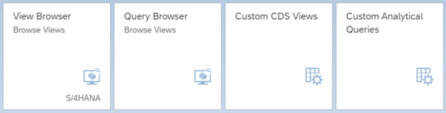
As mentioned, in SaaS version S/4, tiles are all you have. For the work described in this chapter, the four tiles shown in Figure 4-1 are your friends.
Figure 4-1
Tiles for apps used in the process of developing analytical queries in a SaaS-compatible manner
The app View Browser is the best way to explore SAP-delivered CDS views of all types. The view Query Browser can be used in many ways such as to discover SAP-delivered analytical queries and to test-drive analytical queries, either SAP-delivered or custom. However, the app can also be used to give access to analytical queries in a productive environment. The apps Custom CDS Views and Custom Analytical Queries are the SaaS options for developing custom analytical queries and underlying composite views. All these apps will be covered in the upcoming sections of this chapter.
Discovery of SAP-Delivered CDS Views with Tiles View Browser and Query Browser
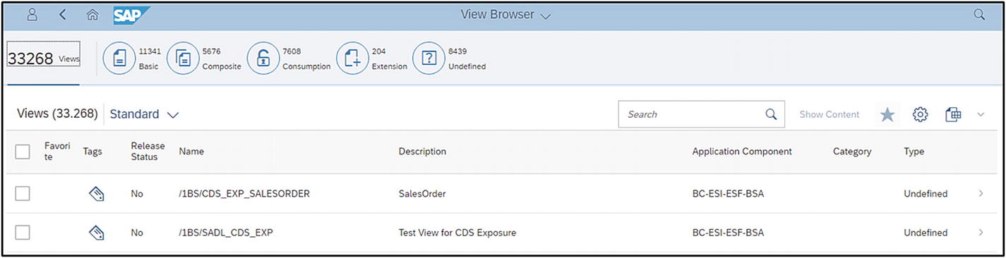
I definitely have spent a lot of time browsing for standard SAP views, and I have reached the conclusion that the app delivered by SAP for this purpose is the best way to do this. Clicking the View Browser tile leads to the initial view shown in Figure 4-2. Nothing is in the search bar yet, so the list and the statistics shown are for all CDS views in the system, standard as well as custom. Views are ordered alphabetically by name, which is why the first ones are funny ones starting with slashes. The Release Status column specifies whether the view can be used in a SaaS environment. Views with the release status Yes are also called whitelisted.
Figure 4-2
Initial view after opening the app View Browser
But now, how do we effectively use the search bar? Let me start with a practical pointer for SAP dinosaurs like me: do not use asterisks. It took me several months to break this habit. It is a Google-like search method: the search string is looked for in all parts (beginning, middle, end) of all aspects (name, description, properties) of the CDS view. The result set of the search is often larger than what you might have hoped for, but on the bright side, it is hard to miss something this way.
Then what do we put into the search bar? You can of course use the old-school German abbreviations for table names, like BKPF (Belegkopf für Buchhaltung) or BSEG (Belegsegment Buchhaltung), or field names, like BUKRS (Buchungskreis) or GJAHR (Geschäftsjahr). Yes, with old-school SAP it helps a lot if you speak a little German. But then you will mainly find more basic CDS views that still use the original table and field names. The SAP developers of CDS views seem to have a tendency to replace the short, German-based abbreviations for table and field names with longer English-based names like CompanyCode or FiscalYear. To find less basic CDS views, it is therefore better to use such English-based names.
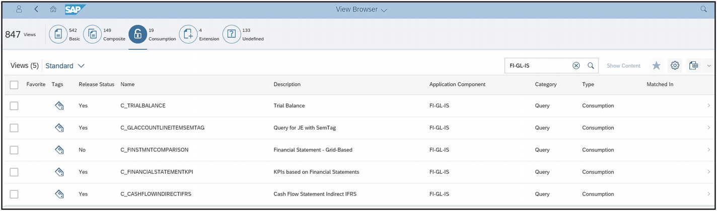
Let’s jump to the search method I like most. Your interest will usually be in a specific reporting domain like Inventory or General Ledger Accounting. During initial searching on field names and other terms, you will find results within a specific application component. For CDS views within the General Ledger Accounting domain, for example, you will notice that the views lie within an application component named FI-GL-IS. Entering this in the search bar gives you all the CDS views relevant for this type of reporting. Figure 2-3 shows the search results using this method; there are 847 views of which 542 are Basic, 149 are Composite, and 19 are Consumption. That’s a large number of views, but user-friendly filtering options are available. For example, clicking the Consumption icon and filtering on a column Category equal to Query gives the result set of the five views shown in Figure 4-3.
Figure 4-3
Search results in the View Browser app using the application component as a search term
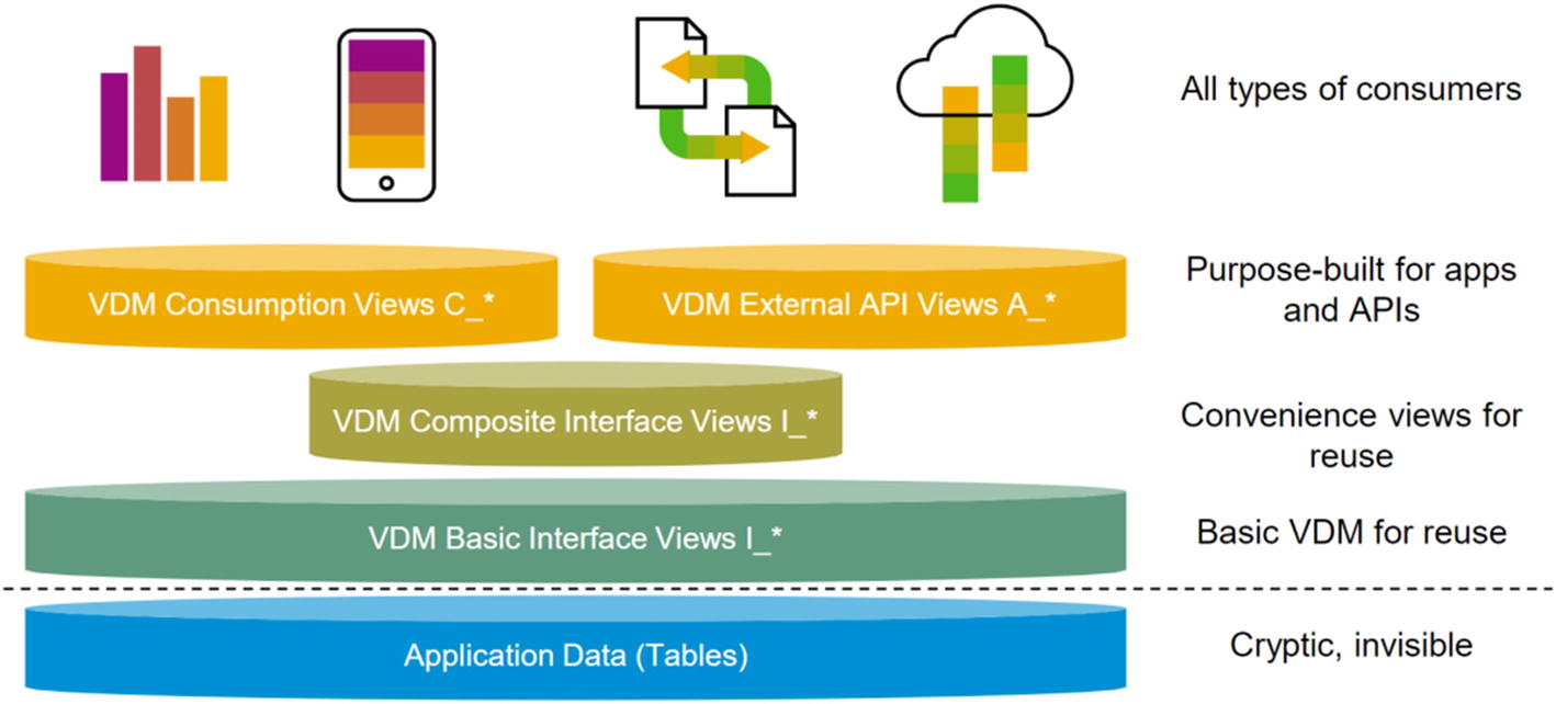
Let’s take a moment to plot all the different types of CDS views in the data modeling layers of Figure 1-3 in Chapter 1. Remember the raw-data layer, data-integration layer, cube layer, and query layer? What SAP calls Basic views can be plotted in the lowest part of the data-integration layer, directly above the physical tables. Composite views are also in the data-integration layer, except for composite views of type Cube, which belong in the cube layer. Finally, Consumption views of type Query constitute the query layer. For brevity, I will often use the term query view for Consumption views of type Query, and cube view for Composite views of type Cube.
SAP applies the following naming convention for the standard CDS views: Basic and Composite views start with I_, where the I stands for “interfacing” referring to the role these views play between physical tables and queries. Consumption views start with C_, where the C stands for…well, “consumption,” of course. There is a group of standard CDS views starting with P_, where P stands for “private.” These are not meant to be reused, so I propose not to reuse them. Finally, there are views of type Consumption starting with A_, with A standing for “API.” These views are meant for external use. In the final chapter, APIs are covered in more detail. Figure 4-4 shows a graphical overview of these different types of views including their naming conventions.
The standard CDS views of type Consumption and category Query are particularly interesting, as they are ready-to-use analytical queries. If one exists that matches your requirements, you are done! You do not even have to transport anything, as the SAP-delivered CDS views are part of the software and exist all through your DTAP system landscape. For SAP newbies, DTAP means Development, Testing, Acceptance, and Production. So, please always check if you can take this shortcut. The tile Query Browser can be used to open and test-drive these queries, as shown in Figure 4-5.
Figure 4-5
Search results in the Query Browser app using the application component as a search term
Not by accident, this is the same result set of five views as obtained with View Browser and shown previously in Figure 4-3. Apparently, queries that are not released are available for the app Query Browser and can be used productively. Once again, we bump into a Trial Balance. Let’s focus on this query for a moment.
In Figure 4-6, information details obtained via the app View Browser and the app Query Browser are compared. Both apps present a list of field names with some properties and annotations. The information tab Cross Reference is available only for View Browser. View Browser has a Show Content button, which to be honest does not always work. Query Browser has a Open for Analysis button, which does always work and which kicks off the query as an app of type Design Studio in an environment described extensively in Chapter 2.
Figure 4-6
Information for a CDS view of type Consumption in the category Query via the app View Browser (top) versus Query Browser (bottom)
The information in the Cross References tab via the app View Browser is quite interesting, as shown in Figure 4-7. Usually, there is a long list of views with a master data relation. For a query view, a master data relation is denoted with Relation equal to Left Outer Join, for other views a master data relation is denoted as Association with a certain cardinality. But the most interesting information is the CDS view with Relation equal to From, as this is the underlying view on which the view is primarily based. Using the app View Browser, you can find out that the query view C_TRIALBALANCE is based upon the cube view I_GLACCTBALANCECUBE, which on its term is based upon the view I_GLACCTBALANCE, and so on, and so on, all the way down to the basic views.
Figure 4-7
Information in the tab Cross References via the app View Browser for a query view (top) and an underlying cube view (bottom)
In conclusion, the tiles View Browser and Query Browser can be used to explore the available SAP-delivered CDS views. Query Browser can also be used to test-drive standard query views. In an ideal world, a standard query view exists that matches your requirements, and you are done. If not, you can use View Browser to identify cube views as potential candidates to build custom analytical queries on top of. That brings us to the next section of this chapter.
Custom Analytical Query in an Almost Ideal Situation: Part 1
In an ideal situation, a ready-to-use SAP-delivered query view exists that matches your requirements. In a slightly less ideal situation, no such query view exists, but there is a strong standard cube view upon which a custom query view can be based. I will present that example in this section.
The example involves the most popular business case of all: actual-plan comparison in the financial domain. It is hard to find an SAP ERP system without actual financial amounts, and often planned amounts are also present. The purpose of the latter is to compare the actuals to check whether the income and/or expenses are still within the prediction or budget. The application component for this type of financial data is FI-GL-IS, not coincidentally the example used in the previous section. By now we know we need to search for composite views of type Cube not starting with P_ but with I_. While the app Query Browser can work with unreleased query views, the app Custom Analytical Queries cannot work with unreleased cube views. Applying all relevant filters to the search in View Browser leads to an overseeable list of 17 views, one of which has the promising description “Actual Plan Comparison for Journal Entry Item” and technical name I_ActualPlanJournalEntryItem. Inspecting this cube view via View Browser gives a long list of available fields, which is always a good sign; all the right annotations; and also a long list of associations, which means that the cube view is heavily enriched with master data.
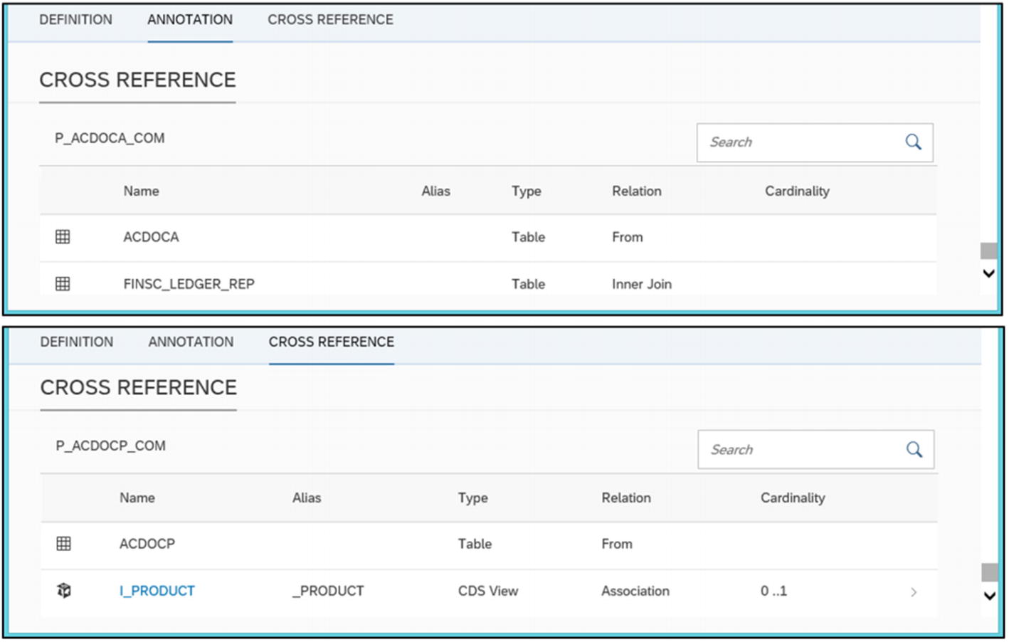
We can now also do the exercise described in the previous section, i.e., using the app View Browser repetitively to find the underlying views via the information on the Cross References tab all the way down to the physical tables. You know you are at the end of this exercise when you see something like what is shown in Figure 4-8.
Figure 4-8
Information on the tab Cross References via the app View Browser for two basic views
Now I want to show you something that will make it absolutely clear that I already was an adolescent during the early days of the computer era. I like to make overviews such as the one shown here:
I_ActualPlanJournalEntryItem
|- P_ActualPlanJrnlEntryItm (union)
|- I_GLAccountLineItem
| |- P_Acdoca_Cube
| |- P_ACDOCA_COM
| |- acdoca
| |- finsc_ledger_rep
|- I_FinancialPlanningEntryItem
|- P_ACDOCP_COM
|- acdocp
You can laugh if you want. But this text-style overview does have the advantage that you can add it to all kinds of documents as well as inline comments in your code. By the way, it works best with a monospaced font. The overview clearly – yes, clearly - demonstrates the layered structure of CDS views from the cube view down to tables. The main tables in this setup are the relatively new Simple Finance tables Universal Journal Entry Line Items (ACDOCA) and Plan Data Line Items (ACDOCP). Simple Finance is a term we are not allowed to use anymore by SAP, but I am a rebel. Universal Journals combine information from various types of financial documents (Finance, Controlling, Profit Center Accounting, etc.) from the pre–Simple Finance era, which implies that ACDOCA combines data from tables such as Accounting Document Segment (BSEG), CO Object: Line Items (by Period) (COEP), and more. Planning data also used to be scattered across the entire database but is now neatly combined in the table ACDOCP. In conclusion, the table content, on which this cube view is based, is excellent for our purposes.
We can also see that this stack of CDS views is not something we can build ourselves with tile Custom CDS Views. The only data modeling option this app has to offer is adding associations, which technically are left outer joins. This stack of CDS views has a view applying the union operator to combine the Actuals and Plan key figures, and inner join clauses are applied as well, e.g., to join the ACDOCA and FINSC_LEDGER_REP tables. If unions, inner joins, or aggregations via the GROUP BY clause are required in the data model, the only thing you can do in a SaaS environment is hope that SAP has done this for you in one of its standard CDS views or will do so in future releases.
But this time we are lucky. The cube viewI_ActualPlanJournalEntryItem looks like an excellent basis for our financial actuals-plan comparison report. So, let’s get started. First we’ll see how far we get using only the tile Custom Analytical Query. Click the tile, and a screen appears as shown in Figure 4-9. It contains a list of existing views of type Consumption in the category Query, most of which are SAP-delivered. As we want to build a new query, click New. A mandatory prefix is something like YY1_ or ZZ1_, depending on the system settings. As the data source is named I_ActualPlanJournalEntryItem, I would have preferred to name the analytical view ZZ1_ActualPlanJournalEntryItem, but that is too long. The name ZZ1_ActPlanJEItem works. Click OK to continue.
Figure 4-9
Custom analytical queries: starting and entering the basics
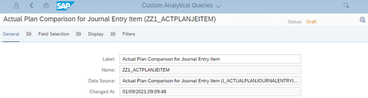
The next screen is explains the development process with arrows urging us to go from left to right: General >>> Field Selection >>> Display >>> Filters. On the General tab, we only need to fill in a label for the query (Figure 4-10).
Figure 4-10
Custom analytical queries: General tab
The tab Field Selection is where we can pick our fields (Figure 4-11). The standard cube view offers 170 (!) fields to choose from. I want to keep it simple and high level, so I pick only two amounts and the high-level characteristics Company Code, Fiscal Year and Fiscal Period, Ledger, and Profit Center. The characteristic Category (PlanningCategory) is used in table ACDOCP for a planning version, so I need that as well. I had some difficulties finding the field for Account, so I used the available search bar on the left.
Figure 4-11
Custom analytical queries: Field Selection tab
The tab Display shows that by default key figures are placed in columns and characteristics as free characteristics (Figure 4-12). Without modifications, the initial display of the query will show one record with two columns with amounts and no dimensions. I want the initial display to show GL Account in rows, so I change that. Other things I could do in this tab are change the label, add a results row, or change the default display format (key, text, or both), but I will leave everything at the defaults for the moment. For key figures there are other options, but I will leave these at the defaults as well.
Figure 4-12
Custom analytical queries: Display tab
Onward to the next tab: Filters (Figure 4-13). There are a few things I need to do here. First, I need to filter on one specific ledger; otherwise, all the amounts are doubled or tripled. I also add user input filters on Company Code and Fiscal Year, using different options: single value or interval, single or multiple selection, optional or mandatory, with or without default value. Let’s see how these filters work out in practice.
Figure 4-13
Custom analytical queries: Filters tab
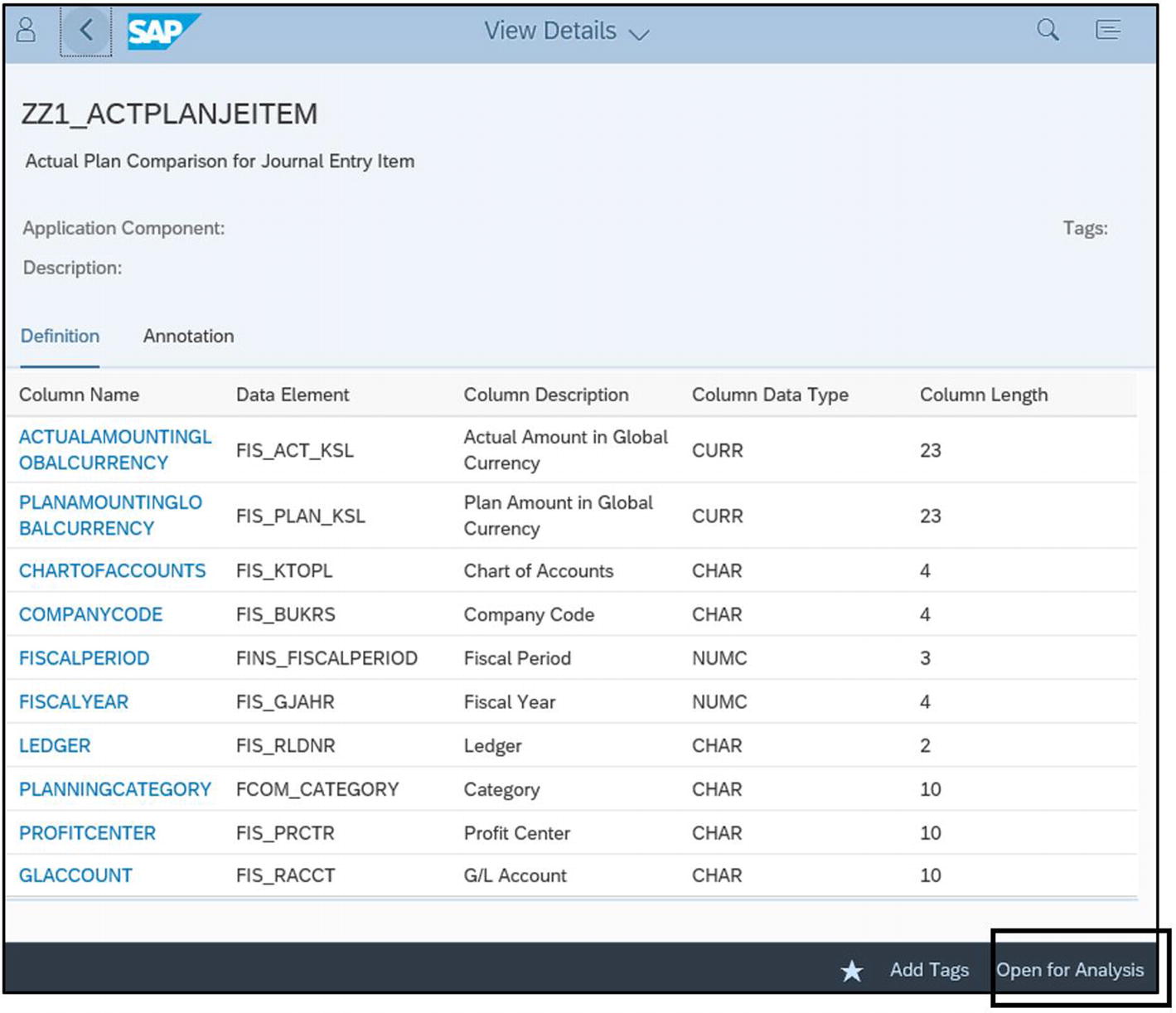
We can now test-drive the analytical query with the tile Query Browser. The View Details screen gives an overview of all the selected fields with some metadata (Figure 4-14). As mentioned earlier, the column name in standard SAP cube views or query views is always different from the technical name of a field in a table, but the data element often gives away the source of the field, as this does not change when traveling from the table via the basic view to the cube view and the query view.
Figure 4-14
Test-driving the custom analytical query via the app Query Browser: View Details screen
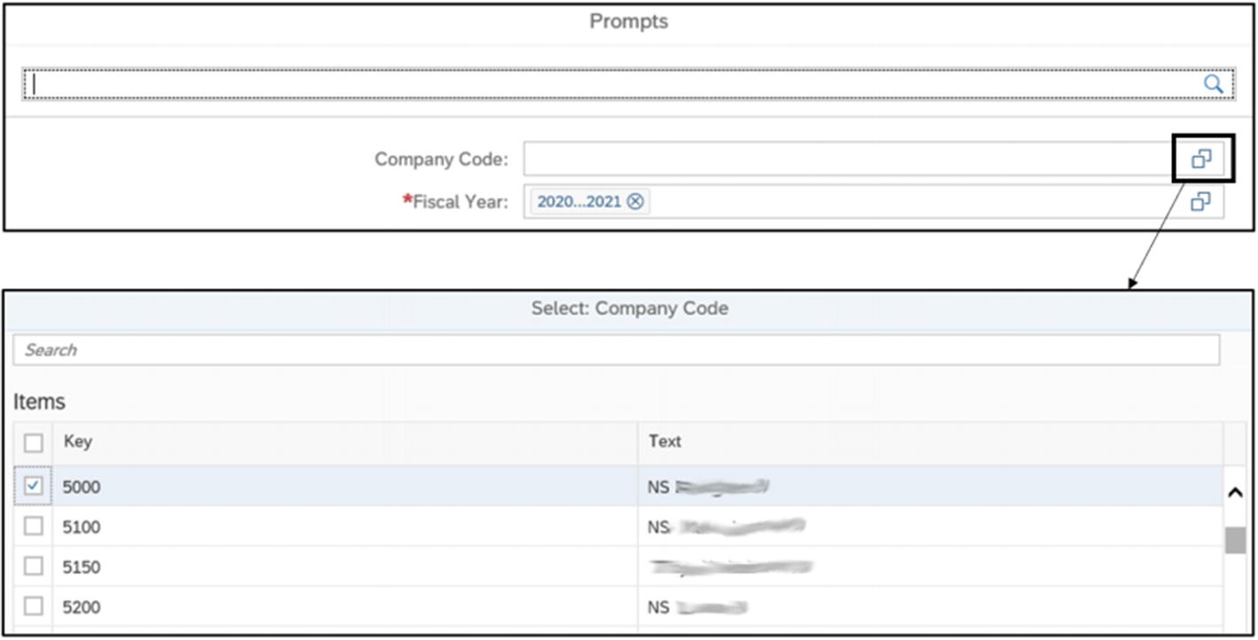
Clicking the button Open for Analysis brings us to the next step: the selection screen (Figure 4-15). It looks perfect. Filter on Fiscal Year has a star, meaning it is mandatory. The default values are filled in, but these can be overwritten. You can select multiple single values for Company Code. There’s nothing to improve here. Let’s click OK and move on.
Figure 4-15
Test-driving the custom analytical query via the app Query Browser: selection screen
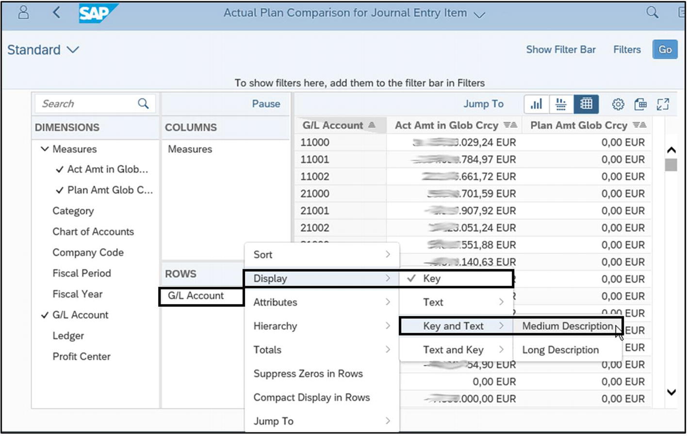
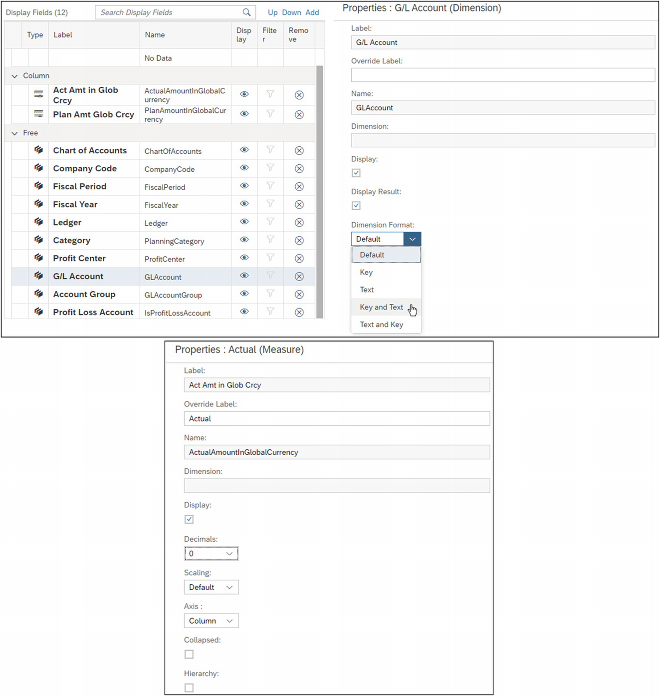
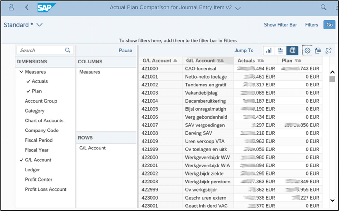
The next screen shows the initial display of the query result: Actual and Plan amounts in the columns and G/L Account in the rows—so far so good (Figure 4-16). But there are some features I do not like. Apparently the default format option for characteristics is the key only. A user can switch that to key and text, but it would be preferable to have that format as an initial display for G/L Account, Company Code, and Profit Center.
Figure 4-16
Test-driving the custom analytical query via the app Query Browser: initial query output
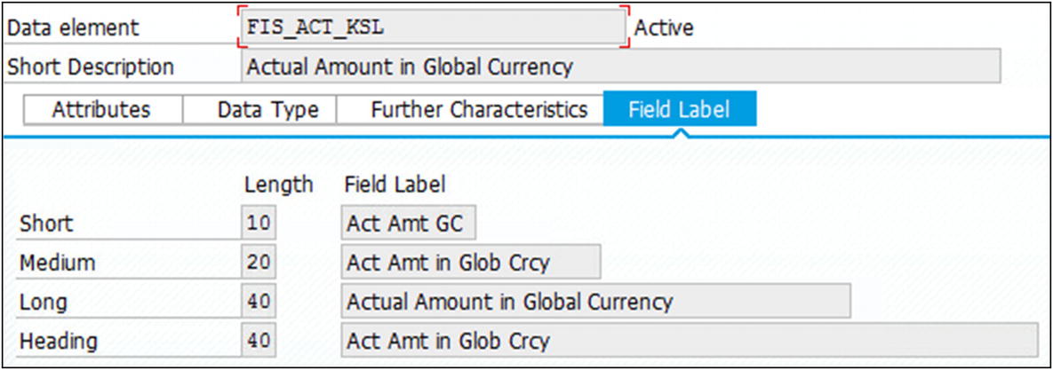
For the key figures, I also see some potential optimizations. First, I would like to get rid of the euro cents. Second, let’s work on the labels. The actual amount is named Actual Amount in Global Currency on the View Details screen, and Act Amt in Glob Crcy in the query output itself. The latter is an ugly name. Figure 4-17 shows where these descriptions come from. Unless a description is overwritten between the table and cube view or query view, descriptions are delivered by the data element. The View Details screen shows the property Short Description of the data element, and the query output shows the Field Label version of length 20. Overwriting the label in the custom analytical query only affects the query output, not the View Details screen.
Figure 4-17
Source of field descriptions in CDS views
I also need to do something about the planning versions. The dimension Category has the value ACT01 for Actuals and values like PLN or similar for Plan. I need to filter on ACT01 plus one of the planning versions to avoid all planning versions being summed up.
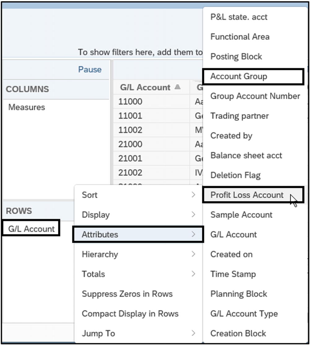
Checking the attributes of G/L Account, I find two of them particularly interesting: Account Group and the indicator Profit Loss Account (Figure 4-18). These are already available as attributes in this version of the query thanks to all the master data associations in the standard cube view, but I would like to use them more dynamically for filtering and separate drilldown, in other words, as a dimension. The query output now starts with balance accounts, and users will often not be interested in those accounts, only in profit and loss accounts. The indicator Profit Loss Account can be used to filter this out. Up to this point, all optimizations I had in mind could be dealt with in the app Custom Analytical Query, but for adding the attributes as dimensions, we need the app Custom CDS View.
Figure 4-18
Test-driving the custom analytical query via the app Query Browser: checking the attributes of G/L Account
Custom CDS View in an Almost Ideal Situation
We are hands-on types of people, so let’s click the tile Custom CDS View to see where this brings us. It brings us to the screen shown in Figure 4-19: a list of existing CDS views and a Create button.
Figure 4-19
Custom CDS Views screen: starting the app for a new CDS view
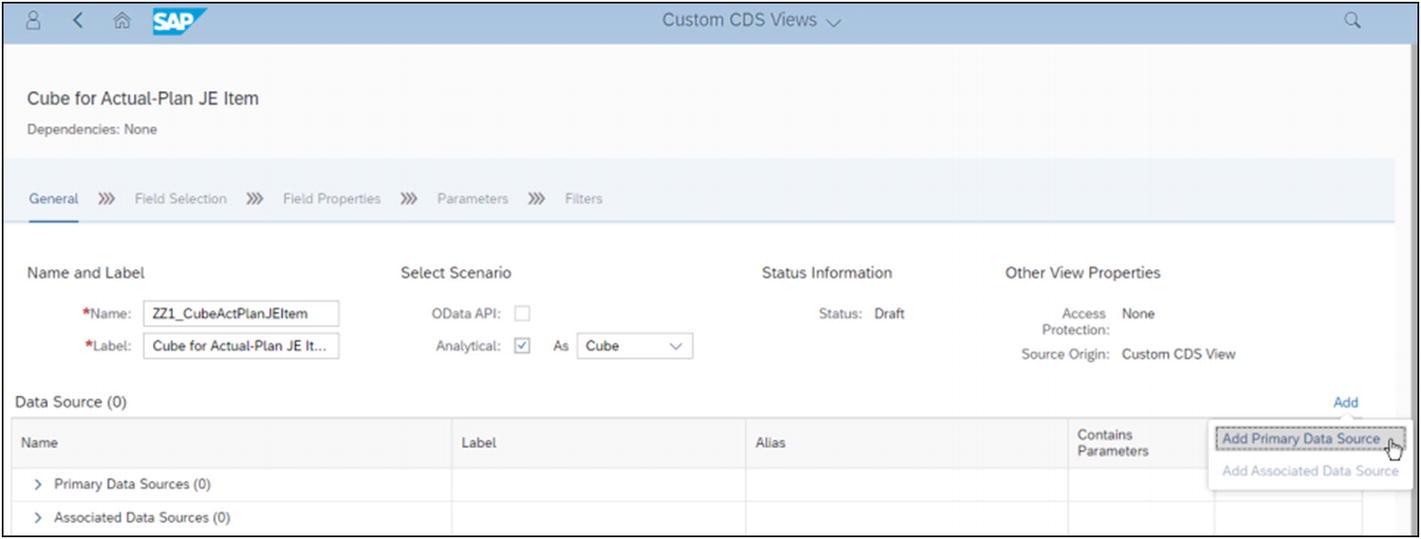
Once again, the first screen explains the development process with arrows going from left to right: General >>> Field Selection >>> Field Properties >>> Parameters >>> Filters. On the General tab, we need to fill in a label, decide whether this view is for external (OData API) or internal (Analytical) use, decide whether the view will be of type Cube or Dimension, and choose a primary data source to start with (Figure 4-20). In this app we can build a cube view connecting facts to dimensions. But in this almost ideal situation with a very rich standard cube view being available, I only want to slightly modify this cube view for our purpose. I therefore choose the cube view we used for the first version of the custom analytical query as a primary data source, I_ActualPlanJournalEntryItem.
Figure 4-20
Custom CDS Views screen: General tab, adding the primary data source
On the next screen, Field Selection, we are in for a surprise (Figure 4-21). Building a cube view on top of a rich standard cube view, we apparently have a staggering number of 48,492 (!) fields and associations to choose from. Most of these are fields via associations (via associations…via associations…), so you may want to use the search bar on the left side. On the right side, you see some key fields that cannot be left out of the custom cube view. These are the key fields of the ACDOCA and ACDOCP tables. Not to worry: they can be left out of the query view.
Figure 4-21
Field Selection tab: using the search bar
There are a couple of things we need to do:
1.
Find and select all the characteristics we need for the query. Ledger, Fiscal Year, and Company Code are already in as they are key fields. Profit Center, Category, and G/L Account need to be added. G/L Account has Chart of Accounts as a compounding key, and it’s the same for Profit Center and Controlling Area, so these need to be added as well.
2.
Select not only the required key figures but also the accompanying currency and unit fields. In our case, this means also select the currency field Global Currency.
3.
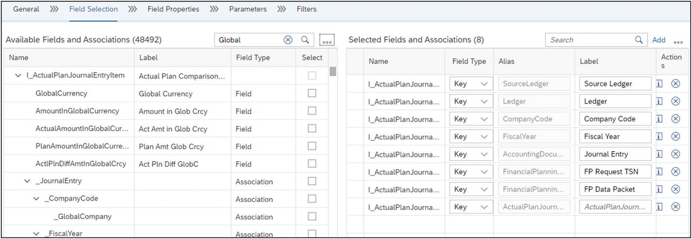
Select Account Group and the indicator Profit Loss Account from the association I_GLAccountInChartOfAccounts, renamed as _GLAccountInChartOfAccounts. The same association appears on many levels in cube views like this one, so it is important to use the association directly below the primary data source. In Figure 4-22 this means the bottom one for Account Group, not the top one.
4.
In the version of the analytical view built directly on top of the standard cube view, we had attributes and text available for Company Code, Profit Center, and G/L Account. But we will lose this functionality, unless we propagate the accompanying associations further in our custom cube view. To achieve this, we need to select the associations_CompanyCode, _ProfitCenter, and _GLAccountInChartOfAccounts. Once again, be careful to pick the right ones (Figure 4-22).
Figure 4-22
Field Selection tab: selecting associations and fields from associations
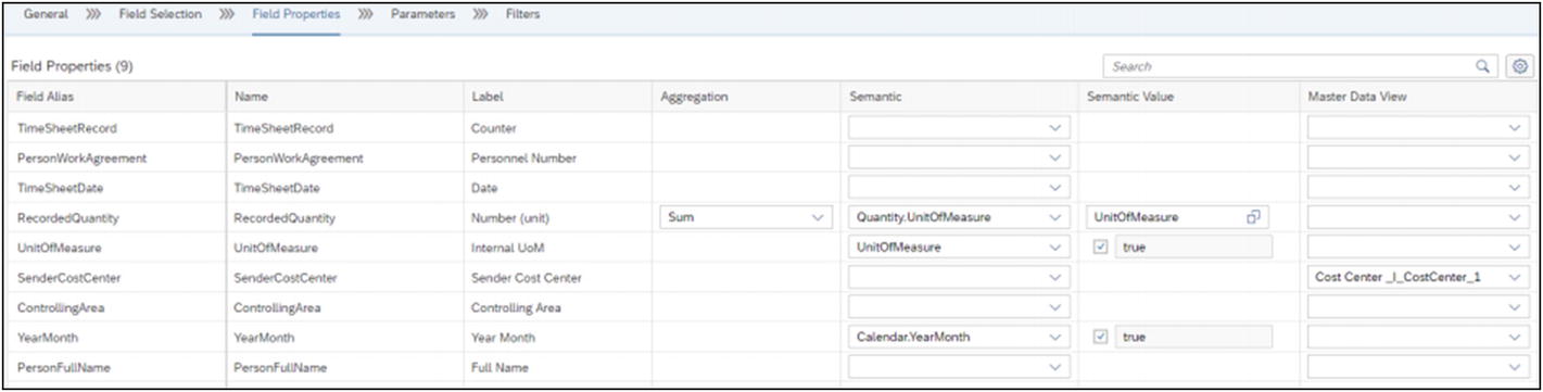
The next step in the development process is the screen Field Properties. Figure 4-23 shows the things you can do in this screen. The column Aggregation is required for all key figures. Usually you fill in the sum for amounts and quantities and the max for things like prizes. The columns Semantics and Semantic Value couple the field to useful metadata, e.g., a couple of key figures to the appropriate currency or unit field. In the column Master Data View, the accompanying view for attributes or text needs to be entered to have attributes or text available in the query.
Figure 4-23
Field Properties tab: options for Aggregation and Semantic
There are two more steps in the development process to cover: Parameters and Filters. As we do not need parameters, and I want to do the filtering in the query view, so we can skip these steps for now.
In hindsight, we did not need the option Add Associated Data Source. This is of course because the primary data source in this case already had so many associations—rather too many than too little.
Custom Analytical Query in an Almost Ideal Situation: Part 2
Let’s go back to tile Custom Analytical Query to implement the optimizations. Ideally, we would change the data source for query ZZ1_ACTPLANJEITEM from I_ActualPlanJournalEntryItem to ZZ1_CubeActPlanJEItem, but as this is not possible, we will build a new query, ZZ1_ACTPLANJEITEM2, on top of cube ZZ1_CubeActPlanJEItem. The number of available fields is now 19 instead of 170, which makes it rather easy to find the required fields. The new field Account Group and the indicator Profit Loss Account are indeed available. On the screen Field Properties, we make the desired changes: set the standard display format of G/L Account to Key and Text and change the label and number of decimals for the two amounts. See Figure 4-24.
Figure 4-24
Field Properties tab: changing the properties of characteristics and key figures
On the Filters screen, we introduce a filter on the new indicator Profit Loss Account. The indicator has a value of X for profit and loss accounts versus ‘ ’ for balance accounts (Figure 4-25). I choose the filter to be mandatory and multiple single values with a default value of X. This way, if the user does not change this in the selection screen, only profit and loss accounts will be shown, but the user has the option to change this to only balance accounts or to both types of accounts. We also introduce a fixed values filter on the dimension Category.
Figure 4-25
Filters tab: filter on indicator Profit Loss Account
It’s time to test-drive the optimized query by starting Query Browser. The selection screen now has an additional entry for the indicator Profit Loss Account, which does what it is supposed to do (Figure 4-26).
Figure 4-26
Test-driving the optimized custom analytical query via the app Query Browser: selection screen
The output of the optimized query looks good as well. All the optimizations are there: key and text for G/L Account, Company Code, and Profit Center; simplified labels for the amounts; no more euro cents; and new dimensions Account Group and Profit Loss Account (Figure 4-27). We are done!
Figure 4-27
Test-driving the optimized custom analytical query via the app Query Browser: query output
Custom CDS View in a Not-So-Ideal Situation
We are not always lucky. Not always is a rich standard cube view available to modify and build a query upon. In such a not-so-ideal situation, we can try to build a cube view ourselves starting from facts and dimensions. In this section, I describe such an example from practice involving the process of time recording.
The first stop is View Browser. The source of time recording transaction data is the table CATS: Database Table for Time Sheet (CATSDB). Entering the table name in the search bar of View Browser teaches us that the application component for this type of data is CA-TS-S4. This application component has 54 views, including 7 basic, 38 composite, and 8 consumption. There are five views of type Consumption and category Query, but none of them have been released, and, more importantly, none of them is useful. There are five views of type Composite and category Cube, but none of them has been released. The best chance of success is the released view Time Recording Data (I_TimeSheetRecord), with the type Basic and the category Fact.
The output of this basic view will also be quite basic: involved employee with personnel number (catsdb.pernr), sending cost center (catsdb.skostl) as a number, and work date (catsdb.workdate) only as a day but not the week, month, or year. These are things we can fix in the app Custom CDS View. So let’s just do that. By the way, denoting fields in this fashion—catsdb.pernr, [table name].[field name] in small letters—is the exact notation in ABAP CDS as inherited from SQL. You’d better get used to it for the remainder of this book.
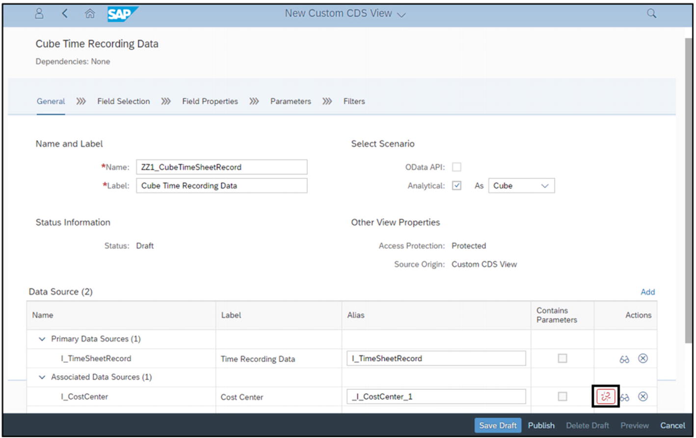
This time we do need to add associated data sources, i.e., the standard CDS views I_CostCenter, I_CalendarDate, and I_WorkforcePerson. While adding a data source, you may need to ignore a warning about adding an access-protected data source. After adding an associated data source, a broken link icon appears (Figure 4-28).
Figure 4-28
General tab: broken link icon after adding an associated data source
This can be solved by entering the correct association properties information. This is shown for Sender Cost Center in Figure 4-29. Do not forget the compounding keys. For the data source I_CalendarDate, the field I_CalendarDate.CalendarDate is connected to I_TimeSheetRecord.TimeSheetDate. For the data source I_WorkforcePerson, the field I_WorkforcePerson.PersonExternalID is connected to I_TimeSheetRecord.PersonWorkAgreement. This may cause a problem, as the field I_WorkforcePerson.PersonExternalID is not a key field, which may influence cardinality.
Figure 4-29
General tab: Association Properties section
Once all the associated data sources are neatly coupled to the primary data source (Figure 4-30), we can move on to the next tab.
Figure 4-30
General tab: all associated data sources successfully coupled to the primary data source
On the Field Selection tab, I select from the primary data source only the fields relevant to demonstrate the enrichment. I also select the association for Cost Center, the field Year/Month via the work date, and the full name of the employee (Figure 4-31).
Figure 4-31
Field Selection tab
The Field Properties tab of the Custom CDS View app has no secrets for us anymore (Figure 4-32).
Figure 4-32
Field Properties tab
We can now save and publish this custom cube view, which is our first one built from scratch. Well, it was almost from scratch since it was built on top of the basic views of the VDM. While saving, we receive the warning “The association _I_WorkforcePerson_3 can modify the cardinality of the result set,” which is not totally unexpected. Such warnings should be taken seriously. You will learn more about these types of issues in the next chapter.
Am I allowed to show my archaic overview for the last time in this chapter? Here is the layered structure of CDS views down to the (main) tables of what we built in this section:
ZZ1_CubeTimeSheetRecord
|- I_TimeSheetRecord
| |- catsdb
| |- E_TimeSheetRecord
| | |- catsdb
|- I_CostCenter
| |- csks
| |- ...
|- I_CalendarDate
| |- scal_tt_date
| |- I_YearMonth
| | |- scal_tt_month
| | |- scal_tt_year
|- I_WorkforcePerson
|- I_BusinessPartner
| |- but000
| |- ...
|- I_HrRelation
|- hrp1001
|- ...
Proof of the pudding for the new custom cube view is of course building an analytical query on top with the app Custom Analytical Query and test-drive it with the app Query Browser. Let’s go through the necessary steps with some shortcuts. In the app Custom Analytical Query, I select only the relevant fields. On the Display tab, I change the label of quantity RecordedQuantity from Number (unit) to Hours. I also change the initial display format of Sender Cost Center to Key and Text and add it to the rows. I change the label of Year/Month to Month and add it to the columns. See Figure 4-33 for the result of these actions.
Figure 4-33
Display tab
Selecting the analytical query in Query Browser and bringing in Full Name as the second dimension in the rows leads to the output shown in Figure 4-34. For the second time in this chapter, we are done!
Figure 4-34
Test-driving the custom analytical query for the not-so-ideal situation via the app Query Browser: query output
Transporting Custom CDS Views and Analytical Queries
Earlier, I mentioned the DTAP system landscape, with DTAP meaning Development, Testing, Acceptance, and Production. This is the most often used setup for an on-premise SAP system. A SaaS system usually has only two versions: one for DTA and one for P.
Transporting custom CDS views and custom analytical queries built via tiles following the D > T > A > P route for on-premise or the DTA > P route for SaaS systems involves two more tiles: Configure Software Packages and Register Extensions for Transport (Figure 4-35).
Figure 4-35
Tiles required to transport custom CDS views and custom analytical queries: Configure Software Packages and Register Extensions for Transport
These tiles are used for all S/4HANA extensions. Custom CDS views and custom analytical queries belong to the so-called In-App Extensions, just as for instance Custom Fields and Logic. You’ll learn more about In-App Extensions in Chapter 7.
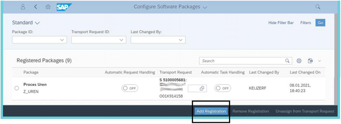
Custom CDS views and custom analytical queries are originally created as local objects, assigned to package $TMP. The tile Configure Software Packages connects an open transport with a task assigned to the developer to a real software package via the Add Registration button (Figure 4-36).
Figure 4-36
The Configure Software Packages tile
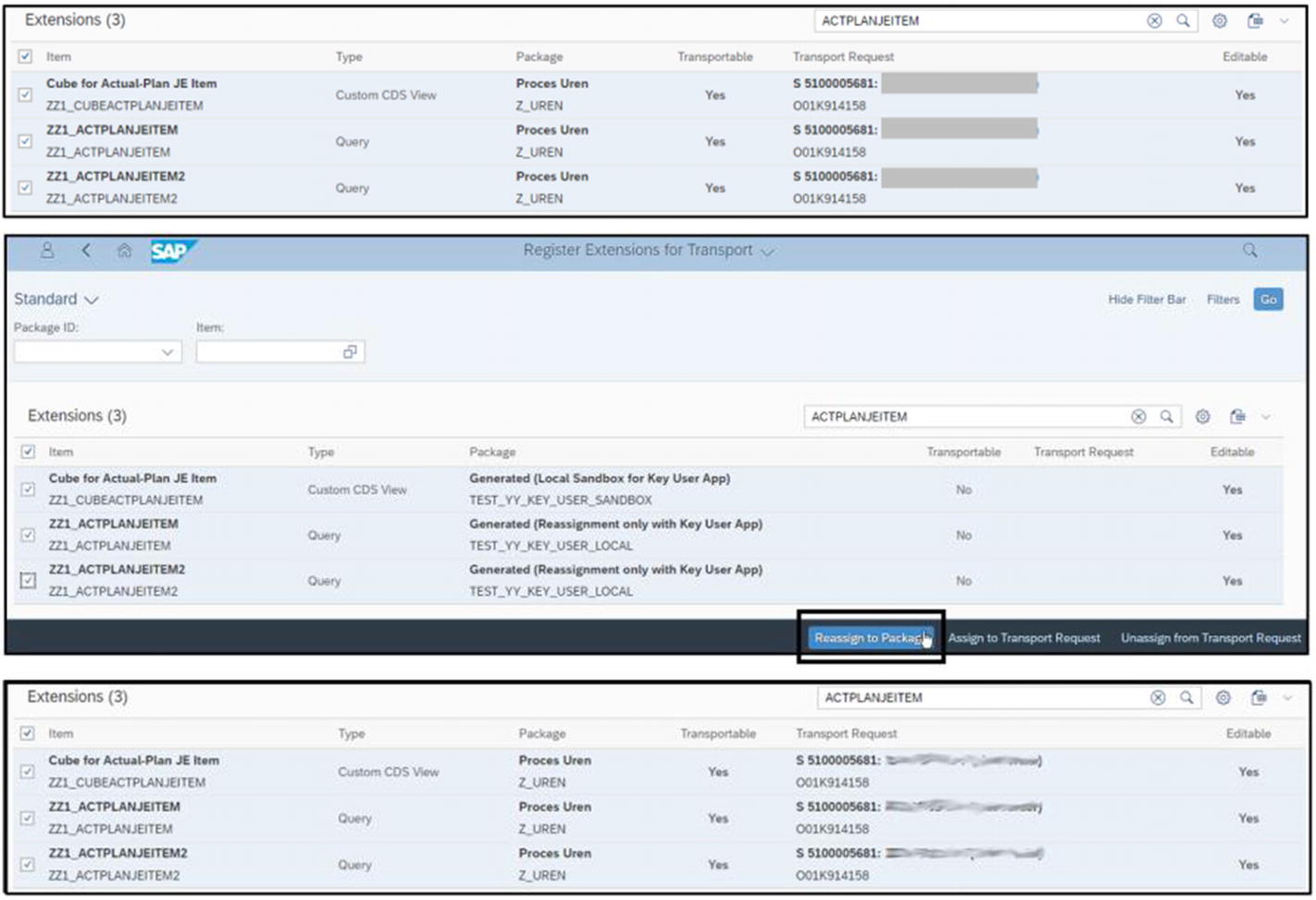
The tile Register Extensions for Transport connects the extensions to the package via the Reassign to Package button. The extensions are then automatically included in the open transport (Figure 4-37).
Figure 4-37
The Register Extensions for Transport tile
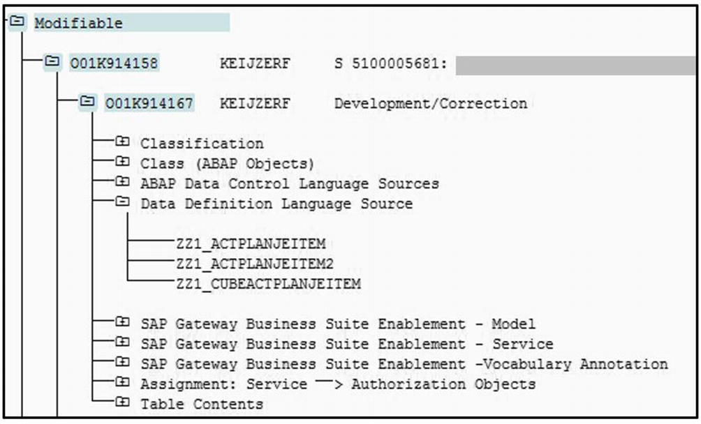
The best way to check the transport for completeness is to check the objects under Data Definition Language Source. Figure 4-38 shows the output of the back-end transaction Transport Organizer (SE01).
Figure 4-38
Contents of a transport including custom CDS views and custom analytical queries (back-end transaction SE01 output)
The objects are now ready to follow the normal transport process of the project.
Retrospective
Allow me to spend some time looking back at what we did in this chapter and drawing some conclusions regarding the usability of the tools presented.
First, let’s look at the not-so-ideal situation example. This example is actually based on a real-life business requirement in a SaaS environment. To be honest, I had a hard time bending the demo around all the issues, e.g., by focusing on the sending side of the data. In reality, we were more interested in the receiving side, but the fields in CATSDB required to report on the receiving side were missing in the basic view. We also wanted to combine the time-recording data with financial data. This required the use of a union operator, which is not possible in a SaaS-version S/4HANA environment. Bummer. The idea back then was to focus on side-by-side extensibility outside of the S/4HANA system. You’ll learn more about this type of extensibility in Chapter 7. And then, all the team members including myself left to do other things, like happens ever so often. So, no, it’s not a success story.
Second, let’s talk about the almost ideal situation example. I started off by explaining the benefits of building analytical queries in this SaaS-compatible way, even in an on-premise environment. Not only are you a goody-goody, but also, as you build the custom objects on top of SAP’s virtual data model of CDS views, upgrade issues are not likely to occur, and if they are, they are SAP’s to solve and not yours. I then shared my enthusiasm regarding this particular SAP-delivered cube view, I_ActualPlanJournalEntryItem. But does this mean that the resulting analytical query is now used in a real-life productive system? I am afraid not. A version of the query similar to what is described in this section is indeed transported into the productive system, but only to compare the performance of this query with that of a similar query built in an IDE (covered in the next chapters). The following are some reasons why the standard cube view in the end did not meet requirements. These reasons are typical for this customer project situation, but the type of mismatches will give you an idea what type of disappointments to expect in your experience with SAP’s VDM:
An extremely useful field like Debit/Credit Indicator (acdoca.drcrk) is renamed to DebitCreditCode in view I_I_GLAccountLineItem, disappears in view P_ActualPlanJrnlEntryItm, and is thus not available in our cube view I_ActualPlanJournalEntryItem. Do you see now how handy my overview is?
In the current project, the process of time recording is done on the level of Network Activity. The following fields in the ACDOCA table are involved in this process: Network Number for Account Assignment (acdoca.nplnr) and Network activity (acdoca.nplnr_vorgn), renamed to ProjectNetwork and RelatedNetworkActivity in view I_I_GLAccountLineItem, disappearing in view P_ActualPlanJrnlEntryItm, and not available in our cube view. For the real-life requirements of the current project, this was a blocking issue.
Some other fields from table ACDOCA were also missing in the cube view; not all of them were critical, but some were.
In principle, table ACDOCA should include an alternative for all the fields from tables like BSEG and BKPF. In reality, some fields from BKPF were required for which there was no alternative in ACDOCA. These fields were also not included in the standard cube view.
Complex logic was required for numerous purposes, e.g., filtering of the dataset on complex conditions involving multiple fields. There was no way this could have been possible within the limitations of the two tiles Custom CDS Views and Custom Analytical Queries.
But I have to admit, for the almost ideal situation example, the SaaS development options have come a long way. And if SaaS is all you have, you are more likely to stretch the available options to the limit than when you can easily move to the on-premise tooling described in upcoming chapters. My final advice to fellow developers working within a SaaS-version S/4 environment is to take a short course in expectation management.