If you are dealing with a SaaS-version S/4HAHA environment, then this chapter and the next are not for you. Sorry. Do not blame me, but blame the person who decided that SaaS was good enough for your organization. Go back to Chapters 3 and 4 to squeeze every last drop of functionality out of the tiles. You also may want to take a look at the section on side-by-side extensibility in Chapter 7.
If you are a hardcore developer dying to start typing code and you decided to skip Chapter 4, then you made a mistake. The functions explained in the previous chapter for the SaaS situation will not be explained again in the chapters about the IDE (or will be only briefly). See Chapter 4 for an explanation of what the coding in this chapter does.
Getting Started with an IDE
An integrated development environment (IDE) is a software application providing facilities to computer programmers for software development. For SAP software, there are basically two IDEs to consider: WebIDE, which is part of the SAP Cloud Platform (SCP), and Eclipse. WebIDE is cloud-based and thereby the future-proof choice. But at this point in time Eclipse is a more mature platform. I had the opportunity to compare both IDEs when developing HANA calculation views (Chapter 1) and indeed found Eclipse to be much more intuitive for graphical user interface actions such as drawing arrows and connecting dots. CDS view development is mainly typing code, so I can imagine the difference in functionality between the two IDEs being much smaller in that case. The examples presented in this chapter come from an implementation project in which Eclipse is used as IDE.
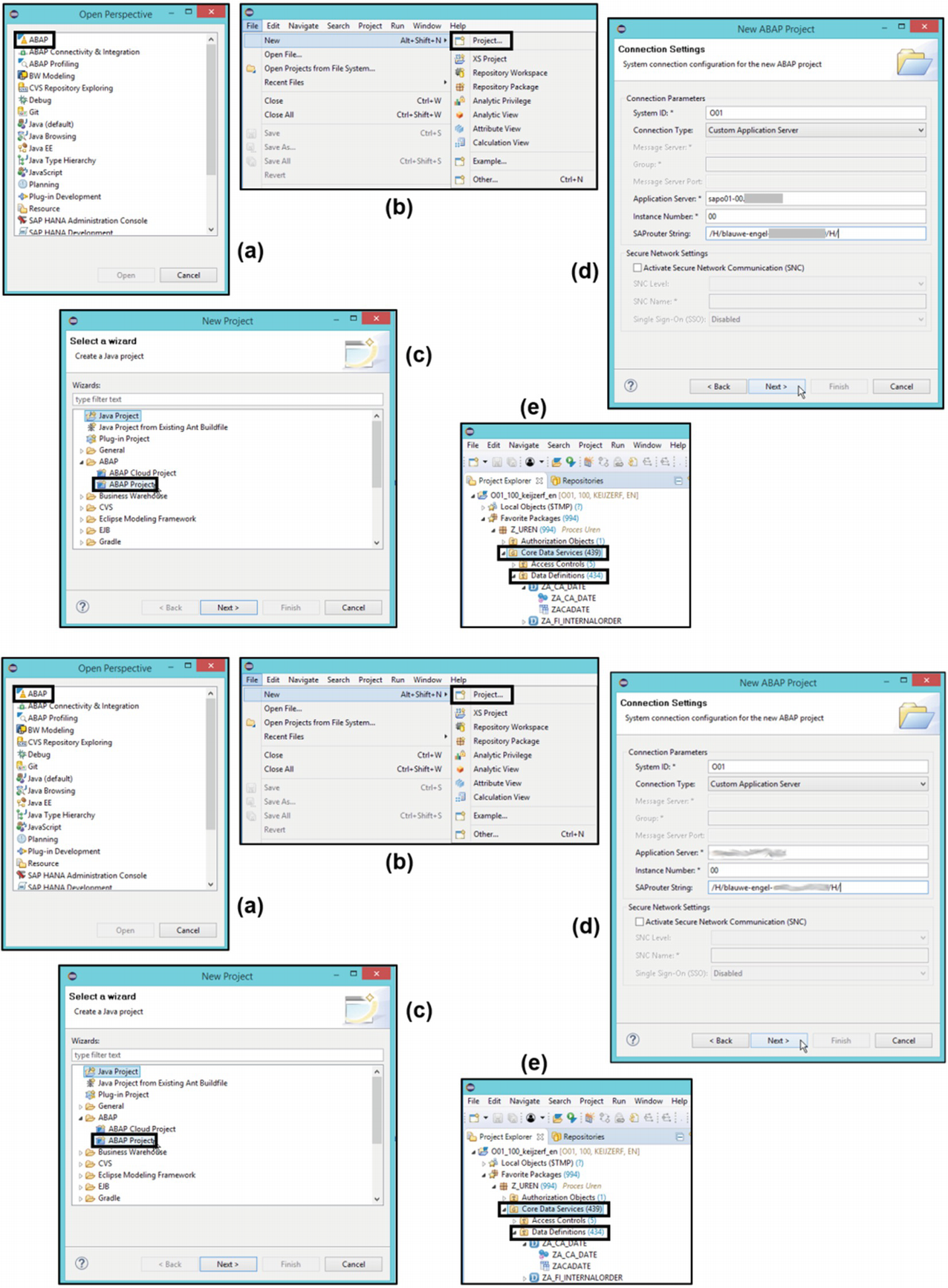
To create custom CDS views in Eclipse, you first need to install the Eclipse software with required the SAP plug-ins or submit an application to the support organization. Once this is done, you can do some preparations, as shown in Figure 5-1. The Eclipse perspective for developing ABAP CDS is the ABAP perspective. Connecting to the S4/HANA development system is done by creating a new project of type ABAP Project, entering the system connection details, and then entering your SAP user credentials. Single sign-on probably does not work, so you may need to change your password in the dev system. The resulting folder structure is [System] ➤ [Package] ($TMP or a real one) ➤ Core Data Services ➤ Data Definitions. Building a custom CDS view comes down to creating a new data definition.
Figure 5-1
Getting started with Eclipse: (a) opening an ABAP perspective, (b) creating a new project, (c) selecting type ABAP project, (d) entering system connection details, and (e) viewing the folder structure
Naming Convention for CDS Views
Referring to the chapter title, is the naming convention for CDS views basic? Yes, the naming convention can be considered basic. It is important to have one from the start and use it consistently, especially when working with multiple developers in the same project. Using it from the start and using it consistently is more important than the naming convention itself. If you cannot think of a good one, then use the naming convention in Table 5-1. Views of type Attribute and Text are mostly Basic, but can also be Composite. View type Data-integration has the Category fact between parentheses, which is not necessarily the case by default. View type Text has the category Text in italics as this is determined by the annotation @ObjectModel.dataCategory, which is an annotation not shown in the app View Browser.
Table 5-1
Proposed Naming Convention for Various Types of CDS Views
View Type
Type in View Browser
Category in View Browser
Example of a Standard SAP View Name
Example of a Custom View Name
Example of a Custom View Description
Query
Consumption
Query
C_MaterialStockTimeSeries
ZQ_MM_RetList
MM: Return List
Cube
Composite
Cube
I_MaterialStockTimeSeries
ZC_MM_RetList
MM: Return List (cube)
Attribute
Basic
Dimension
I_Material
ZA_MM_Material
MM: Material attributes
Text
Basic
Text
I_MaterialText
ZT_MM_Material
MM: Material texts
Data-integration
Composite
(Fact)
P_MaterialStockTimeSeries
ZP_MM_RetListUn
MM: Return List (union)
Basic
Basic
I_MaterialDocumentRecord
ZB_MM_RetListLIPS
MM: Data from LIPS for Return List
The proposed naming convention for CDS views, also used in the current project, is ZX_YY_QqqQqqq. Here, Z is commonly used for custom objects, X indicates the type of CDS view, YY an indicator of the reporting domain (as an SAP veteran I tend to use abbreviations for old-school modules), and QqqQqqq is a unique identifier. In the technical name of the CDS view, it is better to use technical names of tables or fields, for example, rather than language-dependent descriptions. The LIPS part of ZB_MM_RetListLIPS is, for example, the technical name of a table. For a custom description, we chose to start with the indicator of the reporting domain followed by a colon and a functional description, e.g., MM: Data from LIPS for Return List.
Documentation and Data Lineage
So, referring again to the chapter title, is documentation basic? Again, yes it is. If I see a piece of programming, I want to see when it was written, by whom, and why. Often I cannot. The most reliable method of documenting is inline documentation, also known as comments. Documents or spreadsheets have a tendency of getting lost, in spite of or especially in a SharePoint-like environment. Inline documentation is always connected to the code. Just write some information at the start of the code, for instance when it was written, by whom, and why. If you do that, the world will be a better place.
Another important fact often forgotten, but important to be taken into account right from the start, is the data lineage. This is also basic information to include. After 10 layers of CDS views, numerous renamings of fields, and countless transformations, everyone has lost track of the source of the data displayed in an analytical query. A great help would be to add the source of a field as a comment in the lowest basic view and copy that through all the layers up to the query view. It’s surprisingly little work if you do it from the start.
But how can one introduce comments in ABAP CDS? There are two methods.
With /* ... */, everything in between becomes a comment and is ignored as code.
After //, everything on the same line becomes a comment.
Examples of comments for documentation and data lineage will be presented in the “Embedded Analytics from Scratch” sections.
Getting Started with ABAP CDS
How do you learn ABAP CDS coding? Well, this book should be a good start. But as I am the one currently writing it, I had to do without when I started doing this type of work.
The first thing you need is some basic knowledge regarding the SQL language. There are excellent tutorials online, most of them for free (important for Dutchmen, Scots, and so on). The tutorial from w3schools1 is very hands-on and allows you to try things yourself with a database filled with pretty good test data. In fact, I still use it from time to time to explore standard SQL functions.
But regarding ABAP CDS, to be honest I learned most from analyzing existing code and copying parts of it to my custom code. The existing code could be SAP-delivered CDS views. But just as importantly, it could be code generated by the system when building CDS views and analytical queries in a SaaS fashion, in other words, using the tools described in the previous chapter. To show you how instructive this can be, I imported the generated code from the time-recording example in the previous chapter into Eclipse, renamed it in accordance with the proposed naming convention, removed the redundant coding (of which there is quite a lot), reorganized it a bit, and added some structure with comments. I also added the annotation @VDM.viewType, as this annotation is missing after building custom CDS views in a SaaS fashion, which makes the views appear as Undefined in the app View Browser. The following is the result for the cube view:
@EndUserText.label: 'CA: Time Recording (cube)'
@AbapCatalog.sqlViewName: 'ZCCATIMESHEETREC'
@VDM.viewType: #COMPOSITE
@Analytics.dataCategory: #CUBE
@AccessControl.authorizationCheck: #CHECK
@AbapCatalog.compiler.compareFilter: true
@DataAging.noAgingRestriction: true
@Search.searchable: false
define view ZC_CA_TimeSheetRecord as select from I_TimeSheetRecord
association[0..*] to I_CostCenter as _I_CostCenter_1
on _I_CostCenter_1.ControllingArea = I_TimeSheetRecord.ControllingArea and
Going back to Figure 4-29 and Figure 4-30, we recognize the code by the way the fact view I_TimeSheetRecord is connected to the associated data sources _I_CostCenter_1, _I_CalendarDate_2, and _I_WorkforcePerson_3 in the Custom CDS View app. We also recognize the input in the different columns of the Field Properties tab shown in Figure 4-32: Aggregation, Semantic, Semantic Value, and Master Data View.
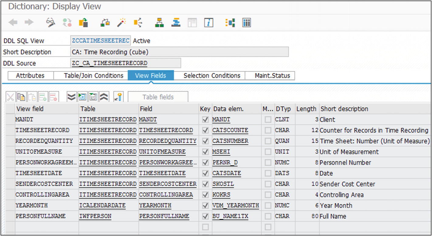
The code starts with annotations. I separated the view-specific annotations from the annotations that are generic for a certain view type. There are two view-specific annotations. The annotation @EndUserText.label is the description of the view as shown before the query output. The annotation @AbapCatalog.sqlViewName is the name of the database view, in other words, the list of fields with properties. It is not allowed to have the technical name of the SQL view be identical to the name of the CDS view. As the naming convention for SQL views, we take the name of the CDS view, remove all the underscores, and abbreviate it a bit if necessary. Therefore, CDS view ZC_CA_TimeSheetRecord becomes SQL view ZCCATIMESHEETREC. You can check both views using the back-end transaction ABAP Dictionary Maintenance (SE11). Enter the name of the SQL view in the search field for View, and a list of fields included in the view will appear, along with other properties (Figure 5-2). The CDS view is shown as DDL source. Clicking the name of the CDS view brings you to a display of the code. Note that by using an S/4HANA back-end transaction you can only display ABAP CDS. To create or change the code, an IDE is required. Displaying the ABAP CDS code via SE11 is a useful method to check the code in a system not connected to the IDE, e.g., the productive system.
Figure 5-2
Display of SQL view via back-end transaction “ABAP Dictionary Maintenance” (SE11)
There are six annotations generic for this view type; five were generated by the system, and one was added by me. The first two, @VDM.viewType and @Analytics.dataCategory, identify the view type. I would not worry too much about the remaining four. You can look them up by Googling them, and you will probably end up in the “CDS Annotations” section of the SAP Help Portal.2 But for me, I am leading a perfectly happy life just copying and pasting annotations without knowing what some of them mean. We will encounter exceptions to my general disinterest in Chapter 6.
Equally instructive, but with less code, is the query view. Again, the annotation @VDM.viewType is added manually.
@EndUserText.label: 'CA: Time Recording'
@AbapCatalog.sqlViewName : 'ZQCATIMESHEETREC'
@VDM.viewType: #CONSUMPTION
@Analytics.query: true
@OData.publish: true
define view ZQ_CA_TimeSheetRecord as select from ZC_CA_TimeSheetRecord
We need to compare this code to the actions carried out with the app Custom Analytical Query, as shown in Figure 4-33, and the result in Figure 4-34. We see the same two view-specific annotations as for the cube view. We also see a different set of annotations specific for the view type. The annotation @Analytics.query: true makes this view appear in the category Query via the app View Browser. The overwriting of labels is done with the annotation @EndUserText.label. The initial display in rows, columns, or neither is achieved with annotation @AnalyticsDetails.query.axis. To obtain an entry in the selection screen, annotation @Consumption.filter can be applied. Initial display as Key, Text, or both is achieved with annotation @AnalyticsDetails.query.display. “A child can do the laundry”, we would say in Dutch.
In the next sections, we will see if we can apply these lessons learned to an end-to-end case based on real-life business requirements.
Embedded Analytics from Scratch: Requirements and Data Model
Sometimes business requirements are as vague as “I want a financial report,” but on the other hand they can also be very specific, as shown in Figure 5-3. This is what a BI consultant can receive if a functional consultant acts as an intermediary. The spreadsheet has two tabs for two different “starting points.” These tabs include a technical table and field names, table relations, and, yes, even input for the selection screen. Never before has a BI consultant been so spoiled! The business requirement had something to do with “clean” and “dirty” parts of trains being returned to a warehouse. Yes, I do like working for the “doink” industry.3 Therefore, this requirement was named “Return List.”
Figure 5-3
Technical translation of business requirements for the “Embedded Analytics from Scratch” case covered in this chapter
Let’s first apply some acceptance criteria to this request. Is it operational information as opposed to tactical/strategic? It is a detailed work list, in which real-time data is much appreciated, so it’s a definite candidate for Embedded Analytics. Does SAP standard content exist to satisfy the requirements or parts of the requirements? Well, as far as the transaction data is concerned, forget about it. But master data is probably available as standard CDS views. The conclusion is that we have to start building.
How do we translate these specifications into a data model? Well, in Chapter 1, we learned that we need to start by searching for the key figures. The data on the tab Starting Point RESB has fields mainly from the table Reservation/dependent requirements (RESB), including the key figures Requirement Quantity (resb.bdmng) and Quantity withdrawn (resb.enmng) and the unit field Base Unit of Measure (resb.meins). The key figure names are easier to memorize once you know that the German word for quantity is “menge.” The tab Starting Point LIPS has one basic key figure, which is coming from table “SD document: Delivery: Item data” (LIPS), i.e., “Actual quantity delivered in stockkeeping units” (lips.lgmng) with the unit Base Unit of Measure (lips.meins).
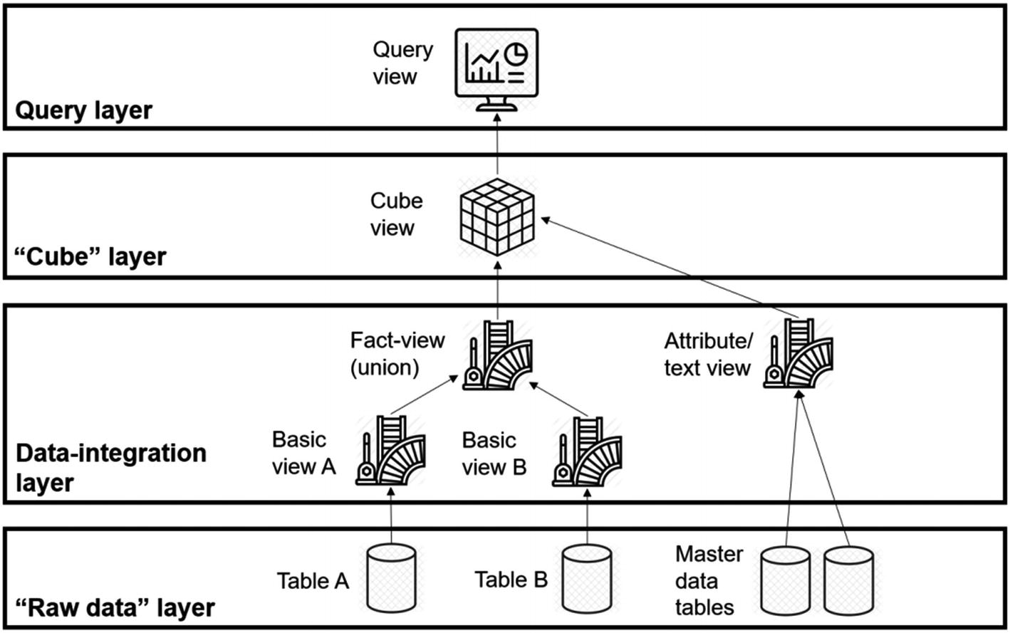
Knowing only this, we already have a basic idea of what the data model should look like. Key figures are coming from two sources not having a one-on-one relation, so we will need a union operator to integrate the transaction data. The data model will therefore look like the one shown in Figure 5-4: two basic views immediately on top of the physical tables, a union view to integrate the transaction data, a cube view, and to top it all off a query view. We have, of course, some attribute and text views, preferably from the SAP standard items, connected to the cube view.
Figure 5-4
Data model for a situation in which transaction data is coming from two sources
There is one thing that worries me in the specifications for the starting point RESB. The requirement to display Delivery and Delivery Item also in relation with the key figures from RESB seems to be at odds with the table relation definition. The definition is that key fields of the primary data source (resb.rsnum and resb.rspos) are connected to nonkey fields of the associated data source (lips.rsnum and lips.rspos). This may lead to cardinality issues, mentioned in the previous chapter. But for now, let’s focus on the basics and revisit this topic later.
Embedded Analytics from Scratch: Basic Views
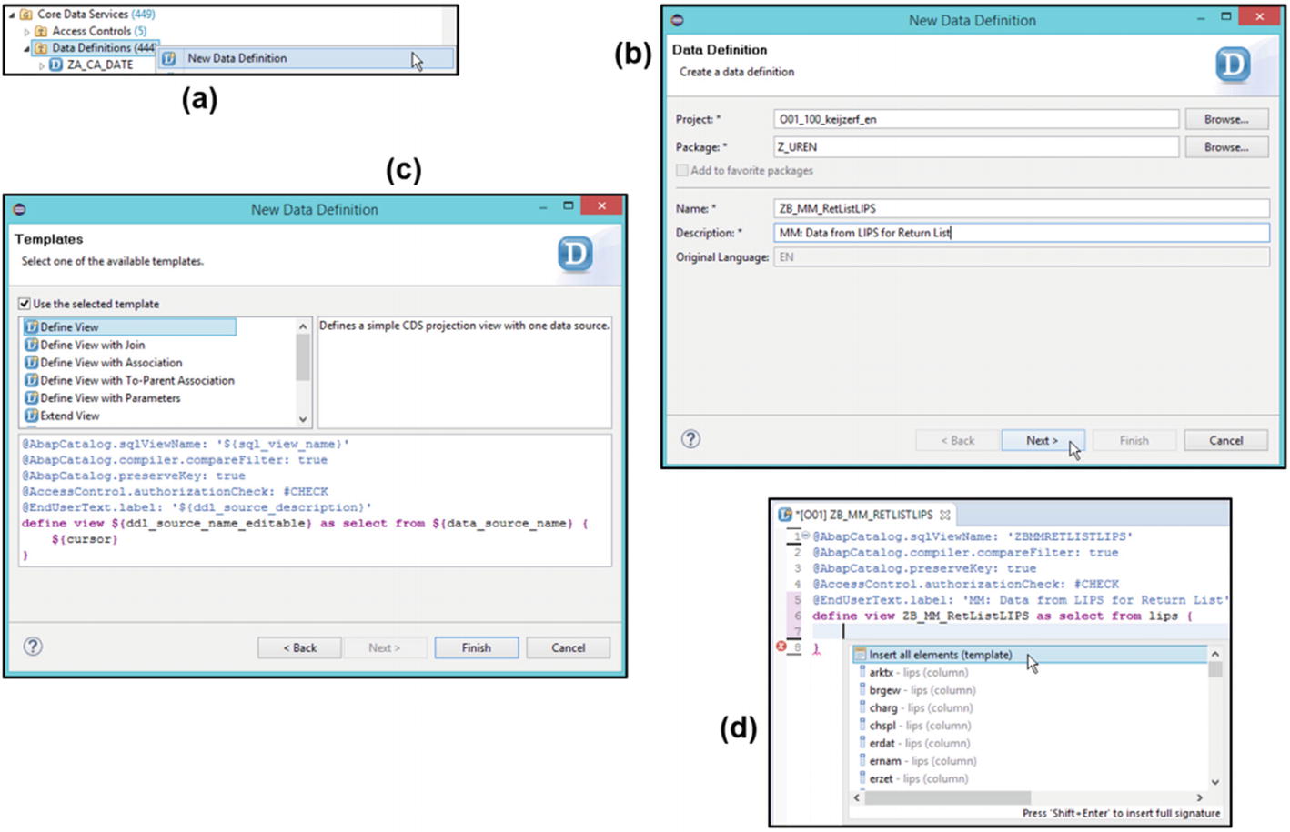
To build a basic CDS view from scratch, nothing in your sleeve, you tell Eclipse you want to create a new data definition, fill in the technical name and description, click Next two times, select the first template you see, and click Finish. The only things you need to do on the coding screen is change the SQL view name from sql_view_name to something else, fill in the table you want to select from, go to a position between the two braces, press Ctrl+spacebar simultaneously (this is the hardest part), and choose the option “Insert all elements” and click Activate (Figure 5-5). There you go, you have created a basic CDS view in less than 10 seconds.
Figure 5-5
Building a basic view from scratch the fast and easy way: (a) create a new data definition, (b) enter the name and description, (c) choose a template, (d) coding screen
Such a CDS view will work, but it will not be pretty. And we also need to add some filters, e.g., on Movement Type. The following is the prettified coding of the basic view for the key figures from the LIPS called MM: Data from LIPS for Return List (ZB_MM_RetListLIPS):
where lips.bwart = '912' and //--Only Movement Type '912' = 'TR transfer in plant'
lips.aufnr != '' //--Order must be filled
On top, you see comments answering the when/who/what/why questions. There is room for a change log for future use. The annotations for the view type were inserted by the template, except for annotation @VDM.viewType, which was entered manually. Data lineage comments are present for every field. This may look a bit redundant at this stage, but it will become more and more useful in the higher architectural layers. Field descriptions and other comments are in English for your convenience, but in the Dutch project they are in Dutch. I have a habit of entering a counter in all basic views and thus at the lowest level, for use during testing, but quite often also in the query. Last, filters are added outside of the braces with a where clause.
The basic view for the key figures from RESB is a bit more complex, as two tables need to be joined. The code for MM: Data from RESB for Return List (ZB_MM_RetListRESB) is shown here:
when lips.vbeln != '' then concat(lips.vbeln,lips.posnr)
else 'XXXXXXXXXXXXXXXX'
end as VbelnPos //Concatenated Delivery Number+Item, special value when empty for testing purposes
}
where resb.rsart = '' and //--Key field "Record type" must be empty
resb.bwart = '531' and //--Only Movement Type '531' = 'Receipt by-product'
resb.aufnr != '' //--Order must be filled
Most of the code will not be a surprise to you by now. This view introduces two SQL statements for the first time in this book: case and concat. The statement case is the SQL method to implement if ... then ... else ... logic. The statement concat is used to attach strings to one another. Please be aware that there is a special statement to attach strings separated by a space, i.e., concat_with_space (this took me a long time to figure out).
You are probably wondering why I am not only counting Reservation Items, but also Delivery Items, and why I am creating a concatenate object from delivery plus Delivery Item. This is preparation for logic we need to implement in the next layer: data integration.
Embedded Analytics from Scratch: Data Integration
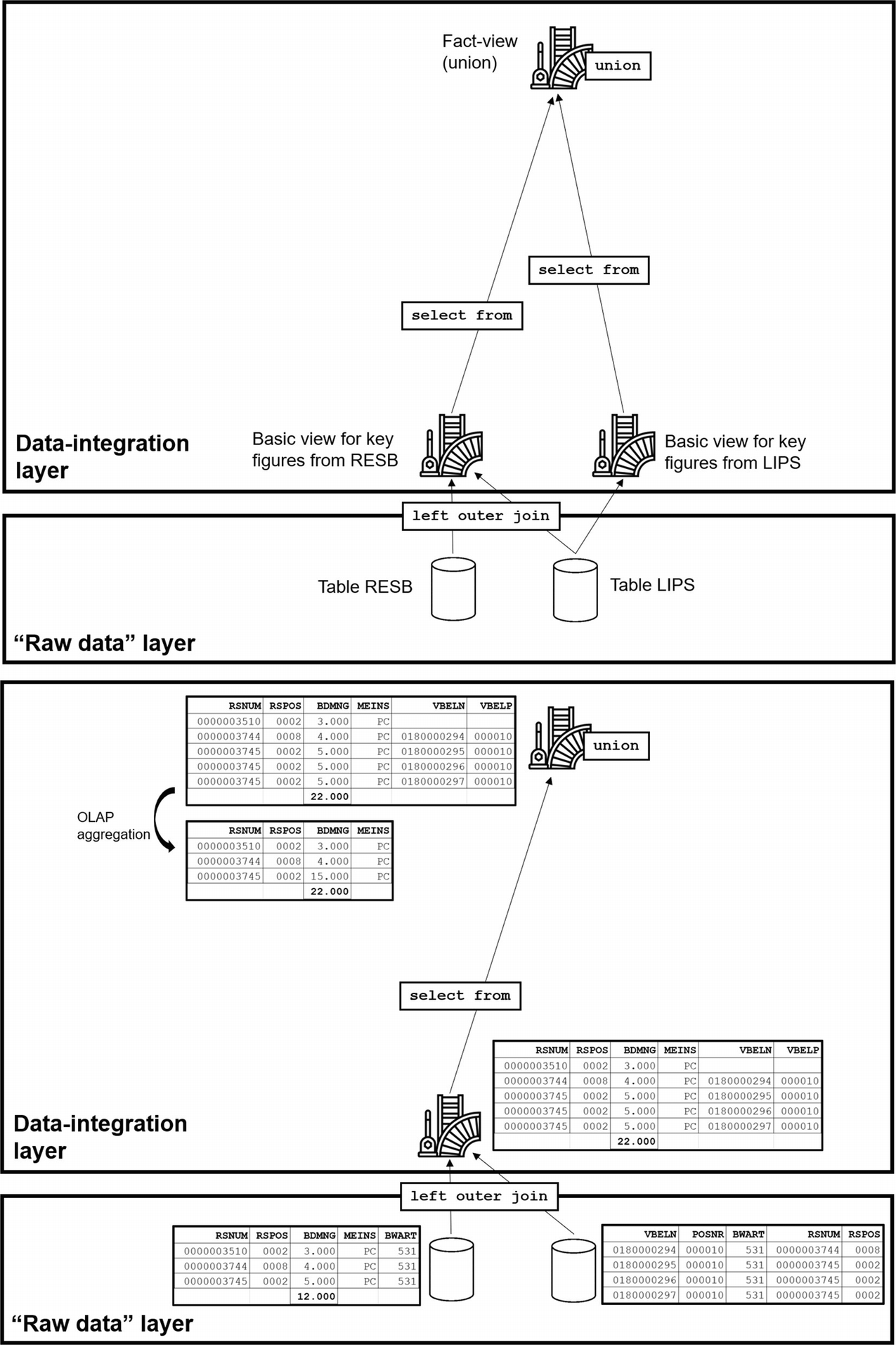
For instructive purposes, let’s act as if we are not aware of the potential cardinality issues in the part for key figures from RESB and continue implementing the data model shown in Figure 5-4. Figure 5-6 shows the result.
In general, left outer joins are used to connect data including key figures on the left side to master data without key figures on the right side. This works well as long as for every record on the left side only zero or one records on the right side are found via the join conditions. This is by definition the case if all key fields of the dataset on the right side are connected to fields on the left side. But our specifications require a left outer join connection between table RESB on the left side and table LIPS on the right side, in which we are not connecting to key fields of LIPS but to other fields. This means there can be more than one record on the right side connected to one record on the left side. In functional terms, for every Reservation Item, there can be more than one Delivery Item, which is very true.
The bottom part of Figure 5-6 gives a data example: Reservation Item 0000003510/0002 is connected to 0 Delivery Items, Reservation Item 0000003744/0008 to 1, and Reservation Item 0000003745/0002 to 3. The result is that the value of key figures from RESB, e.g., Requirement Quantity (resb.bdmng), are tripled for Reservation Item 0000003745/0002 in the basic view and will continue to be tripled all the way up to the query if we do not take action.
Figure 5-6
Demonstration of a cardinality issue. Top: data model. Bottom: display of the data
This can be fixed in the data-integration layer. After all, that is what the data-integration layer is for. In simple cases, it could be fixed with a group by statement in the union view for data coming from the basic view MM: Data from LIPS for Return List (ZB_MM_RetListLIPS). We could, for instance, only keep the highest value of Delivery Item for Reservation Item 0000003745/0002, which is Delivery Item 0180000297/000010, and remove the lines for the other two. But, in consultation with my functional colleague, we decided to not only show the highest value of Delivery Item, but also indicate the fact that there are more than one by counting the number of Delivery Items also for the dataset with key figures from RESB. This is where the preparations in the basic view for key figures from RESB come in handy.
Step 1 in this fix is building a view on top of the view with the cardinality issue to select only one value of the relevant characteristic. The concatenation of Delivery Number and Delivery Item prepared in the basic view is used in this action. Additionality, we want to keep count of the number of Delivery Items. For this we can use the counter that was also prepared in the basic view. The resulting code of view MM: Data LIPS aggr.to Reservation (ZP_MM_LIPSResAg) looks like this:
/* Freek Keijzer, myBrand, 17.01.2021
Preparation for data aggregation of Delivery Items to Reservation Items.
There can be multiple Delivery Items for 1 Reservation Item.
In this view, 1 of these Delivery Items is selected for display
@EndUserText.label: 'MM: Data LIPS aggr.to Reservation'
@AbapCatalog.sqlViewName: 'ZPMMLIPSRESBAG'
@VDM.viewType: #COMPOSITE
@AbapCatalog.compiler.compareFilter: true
@AbapCatalog.preserveKey: true
@AccessControl.authorizationCheck: #CHECK
define view ZP_MM_LIPSResAg as select from ZB_MM_RetListRESB
{
rsnum, //Reservation Number (resb.rsnum)
rspos, //Reservation Item (resb.rspos)
max(VbelnPos) as VbelnPos, //Delivery Number+Item
sum(CounterDel) as CounterDel //Number of Delivery Items in Reservations
}
group by rsnum, rspos //--Aggregation on Reservation Item
Step 2 is creating a composite view that is almost a copy of the basic view ZB_MM_RetListRESB. An inner join with the view ZP_MM_LIPSResAg removes two records as planned, while still counting the correct number of Delivery Items. The code of ZP-view MM: Data from RESB for Return List (ZP_MM_RetListRES) is shown here:
/* Freek Keijzer, myBrand, 17.01.2021
View for key figures Reservations.
Dataset for Delivery Item is being aggregated to level Reservation Item.
For determination "Warehouse EWM/IM?" in next view, this table is joined in this view:
T320 - "Assignment IM Storage Location to WM Warehouse Number"
_Resb.Counter as CounterRes, //Number of Reservation Items
_Ag.CounterDel, //Number of Delivery Items
t320.werks as werks_t320, //IM Plant assigned to WM Warehouse (t320.werks)
t320.lgort as lgort_t320 //IM Storage Location assigned to WM Warehouse (t320.lgort)
}
Step 3 is connecting the view with the removed records to the union view. Figure 5-7 shows the overall fix for the cardinality issue. Looking at the graph, you can probably understand why I call this solution a “triangle,” but it may well be that I am the only person in the world who calls it like this. It is a standard concept taught to me by an experienced SQL programmer during a native HANA development project, but it is equally applicable to the development of CDS views.
Figure 5-7
Fix for a cardinality issue with a triangle. Top: data model. Bottom: display of the data
define view C as
select from A
{
field1,
field2,
field3
...
}
union all
select from B
{
field1,
field2,
' ' as field3
...
}
The list of fields for the combined views A and B needs to be identical. If a field cannot be mapped for one of the two views, a “zero” or “empty” needs to be inserted. Not only that, it needs to be the right type of “zero” or “empty.” To give some examples, ' ' is the right type of empty for a CHAR-4 field, but 0000 is the right type of empty for a NUMC-4 field. 00000000 is the right type of empty for a date field, 0 is usually the right type of zero for a key figure, etc. It takes a while to get used to this, but the IDE will guide you through it with error messages.
It is important to note that the data format of a field is defined only by the first selection in the example before the selection from view A. For example, if a date field cannot be mapped for view A, but it can be mapped for view B, then it will not be sufficient to do this:
define view C as
select from A
{
field1,
'0000000' as date2,
...
}
union all
select from B
{
field1,
date2,
...
}
The date field B.date2 will be available in the query, but it will not behave like a date, e.g., be displayed as 17.01.2021 instead of 20210117. To achieve this, the cast expression from ABAP CDS needs to be applied like this:
define view C as
select from A
{
field1,
cast('0000000' as abap.dats) as date2,
...
}
union all
select from B
{
field1,
date2,
...
}
To bring this work to a minimum, select the view for which the highest number of fields can be mapped first. The cast expression is important, as it is used for all data format transformations.4
Standard SQL offers two union statements: union and union all. The difference lies in whether duplicates are allowed.5 For our purpose, combining transaction data from multiple sources, the union all statement is to be preferred. It also gives much better query performance than the union statement. We learned that the hard way.
Let’s get back to our Return List. Let me first present the code of the union view before discussing it in more detail:
/* Freek Keijzer, myBrand, 17.01.2021
Union-view for integration key figures Reservations & Deliveries.
Business requirement: user-story 34567.
Includes:
- Logic for key figure "Quantity Received?",
- Logic for characteristic "Warehouse EWM/IM?",
- Logic for characteristic "Warehouse Completed?".
bwart, //Movement type inventory management (resb.bwart)
kzear, //Final issue for this reservation (resb.kzear)
matnr, //Material Number (resb.matnr)
meins, //Base Unit of Measure (resb.meins)
bdmng, //Requirement Quantity (resb.bdmng)
enmng, //Quantity withdrawn (resb.enmng)
case
when werks_t320 != '' and spe_gen_elikz = 'X' then enmng
else 0.0
end as QuantRec, //"Received" = "Quantity withdrawn" (resb.enmng) with conditions
vbeln, //Delivery (lips.vbeln)
vbelp, //Delivery Item (lips.posnr)
bwtar, //Valuation Type (lips.bwtar)
@EndUserText.label: 'Warehouse EWM/IM?'
case
when werks_t320 != '' then 'EWM'
else 'IM'
end as StorLoc_EWM_IM, //"Warehouse EWM/IM?" = 'EWM' or 'IM' based on table T320
@EndUserText.label: 'Warehouse Completed?'
case
when werks_t320 = '' and bdmng = enmng then 'X'
when werks_t320 = '' and bdmng != enmng then ''
else spe_gen_elikz
end as StorLocCompl, //"Warehouse completed?", based on table T320 and values resb.bdmng/enmng
CounterRes, //Number of Reservation Items
CounterDel //Number of Delivery Items
}
union all
select from ZB_MM_RetListLIPS
{
'LIPS' as Source, //Source = 'RESB', 'LIPS'
rsnum, //Reservation Number (lips.rsnum)
rspos, //Reservation Item (lips.rspos)
werks, //Plant (lips.werks)
lgort, //Storage Location (lips.lgort)
aufnr, //Order Number (lips.aufnr)
'' as xloek, //Item is deleted
bwart, //Movement type inventory management (lips.bwart)
'X' as kzear, //Final issue for this reservation
matnr, //Material Number (lips.matnr)
meins, //Base Unit of Measure (lips.meins)
lgmng as bdmng, //Actual quantity delivered (lips.lgmng)
lgmng as enmng, //Actual quantity delivered (lips.lgmng)
case
when wbsta = 'C' then lgmng
else 0.0
end as QuantRec, //"Received" = "Actual quantity delivered" (lips.lgmng) with conditions
vbeln, //Delivery (lips.vbeln)
vbelp, //Delivery Item (lips.posnr)
bwtar, //Valuation Type (lips.bwtar)
@EndUserText.label: 'Warehouse EWM/IM?'
'EWM' as StorLoc_EWM_IM, //"Warehouse EWM/IM?" = 'EWM' or 'IM'
@EndUserText.label: 'Warehouse Completed?'
case
when wbsta = 'C' then 'X'
else ''
end as StorLocCompl, //"Warehouse Completed?" based on value "Goods Movement Status" (lips.wbsta)
0 as CounterRes, //Number of Reservation Items
Counter as CounterDel //Number of Delivery Items
}
Here are some observations:
The view is of type Composite, category Fact, as it is the last view with transaction data after the cube view.
The list of fields starts with manual input for a field named Source. My best-practice advice is to always do this, even if it is only for testing purposes or for a power-user version of the query. In a query, it gives immediate insight into from which part of the data model data is coming. BW consultants will recognize this as a field standardly available in multiproviders and composite providers.
We are lucky not to have “empties” or “zeros” in the first view selection, so no cast expression required.
The fields bdmng and enmng have a straightforward mapping to resb.bdmng and resb.enmng, respectively, for the selection from ZP_MM_RetListRESB, but are mapped to a different field, in both cases to lips.lgmng, for the selection from ZB_MM_RetListLIPS. The union view is the ideal place to implement this type of mapping logic.
Three new fields are introduced in this view: the key figure QuantRec and the characteristics StorLoc_EWM_IM and StorLocCompl. Please take your time to compare the logic for these fields with the specifications of Figure 5-3. Coding when werks_t320 = '' or when werks_t320 != '' may require some explanation. In the view ZP_MM_RetListRESB, a left outer join was executed with table T320 for the fields Plant (werks) and Storage Location (lgort). If a match is found with table T320, the warehouse is of type EWM; if not, it is of type IM. We are therefore not interested in any of the values of the record found in T320, only if there is a match or not. Checking the value of werks_t320 is sufficient for this purpose.
Labels can be introduced at any level in the stack of CDS views. The cube view makes the most sense, as all queries built on top of the cube view benefit from the label, but labels can also be introduced at a lower level. Here I chose to label the new fields StorLoc_EWM_IM and StorLocCompl in the union view using the @EndUserText.label expression. The labels are automatically propagated to the higher levels and do not need to be repeated.
As said before, the data-integration layer is where the real magic happens. But for now, it looks like we are done and can move on to the cube layer.
Embedded Analytics from Scratch: Cube View
Most of the hard work has been done in the data-integration layer. In the cube view, we optimize the data for multidimensional reporting. Again, let’s look at the code first and then discuss it. The following is the code for cube view “MM: Return List (cube)” (ZC_MM_RetList):
/* Freek Keijzer, myBrand, 17.01.2021
Cube-view for Return List.
Business requirement: user-story 34567
Main source tables:
RESB - "Reservation/dependent requirements"
LIPS - "SD document: Delivery: Item data"
T320 - "Assignment IM Storage Location to WM Warehouse Number"
Layered structure of CDS-views:
ZC_MM_RetList - Cube-view
|- ZP_MM_RetListUn - Union key figures Reservations
_Ret.bwart as MovementType, //Movement type inventory management (resb/lips.bwart)
_Ret.kzear, //Final issue for this reservation (resb.kzear)
@ObjectModel.foreignKey.association: '_Material'
_Ret.matnr as Material, //Material Number (resb/lips.matnr)
@EndUserText.label: 'Del.nr'
_Ret.vbeln as EWMInboundDelivery, //Delivery (lips.vbeln)
@EndUserText.label: 'Del.pos'
_Ret.vbelp, //Delivery Item (lips.posnr)
_Ret.bwtar, //Valuation Type (lips.bwtar)
_Ret.StorLoc_EWM_IM, //"Warehouse EWM/IM?" = 'EWM' or 'IM'
_Ret.StorLocCompl, //"Warehouse completed?", see logic in union-view
//--Characteristics via associations
_Material.MaterialGroup, //Material Group (mara.matkl)
//--Associations to be passed on to a higher level
_Plant,
_StorageLocation,
_Material,
_MaintenanceOrder,
_MovementTypeText
}
Let’s go through the code from top to bottom:
The cube view is the best place for more comprehensive inline documentation. It is for instance a good place to repeat the source tables used in the basic views and to insert the full layered structure of the underlying CDS views. You remember the old-school overview ridiculed earlier, right?
The view is of type Composite and category Cube. It needs to be of category Cube to be able to build query views on top.
We were lucky to find standard SAP CDS views for the required master data. The views I_Material, I_Plant, I_StorageLocation, and I_MaintenanceOrder were used for the attributes and text. The view I_Movement_TypeText was used for text only. The part of the CDS view between the braces is called the projection area. In this area, we first renamed the involved characteristics from the German-based abbreviations to English-based names used in SAP standard views. An example is _Ret.werks as Plant. In the projection area, associations are coupled to characteristics via the annotations @ObjectModel.foreignKey.association and @ObjectModel.text.association.
Renaming fields to the English-based names used in SAP standard views has the additional advantage that options to use the Jump To functionality from analytical queries will become available. This topic will be covered in the next chapter.
For all key figures, the aggregation behavior needs to be entered in the cube view (or lower) with the annotation @DefaultAggregation. Again, use the value #SUM for quantities and amounts, MAX for things like prizes, and other values in exceptional situations.
Key figures are coupled to currencies or units via the annotations @Semantics.quantity.unitOfMeasure and @Semantics.amount.currencyCode.
Comments for data lineage can become more complex before a union view. Here’s an example for a key figure: //"Quantity" = resb.bdmng or lips.lgmng. Here’s an example for a characteristic: //Plant (resb/lips.werks). And if it all becomes too complicated, use //"Warehouse completed?", see logic in union-view.
To make an attribute from a master data view available as a dimension in the query, that is, with full navigational functionality, we need to include it explicitly in the projection area. Here’s an example: _Material.MaterialGroup.
To be able to use the associations for master data in a query, we need to pass them to a higher level. This is usually done at the end of the projection area.
Basically, this is all you need to know about cube views.
Embedded Analytics from Scratch: Query View and Final Result
And now for the grand finale: the query view. In the query layer, we reap what we sowed in the lower layers. Bring on the code:
StorLocCompl, //"Warehouse completed?", see logic in union-view
MaterialGroup //Material Group (mara.matkl)
}
This is the final CDS view, and thus here are the final observations:
A query view will pop up as being of type Consumption in the app Query Browser through the annotation @VDM.viewType: #CONSUMPTION.
More important is the annotation @Analytics.query: true. This will assign it to the category Query in Query Browser, but, more importantly, it is conditional for the view to be used as an analytical query via the app Query Browser or in any other way.
Operations on key figures such as add, subtract, multiply, or divide can be done in the underlying views and propagated to the query view, but they can also be done in the query view itself. BI specialists will recognize this as being the difference between a “before-aggregation” and “after-aggregation” calculation. We could have calculated the quantity QuantityRemaining as resb.bdmng - resb.enmng in a underlying view, and that would have been “before aggregation.” We now choose to calculate it “after (OLAP) aggregation” using the @DefaultAggregation: #FORMULA annotation. This is an example of a situation in which I first built a similar object using the tile Custom Analytical Query in order to learn from the generated code. We want the key figure CounterRes to be available in the query, but not initially displayed. This can be arranged with the annotation @AnalyticsDetails.query.hidden: true.
We saw an example of using the filter annotation @Consumption.filter earlier in this chapter, but in this code we see more options. The characteristic “Warehouse Completed?” indicates which part of the data is normally relevant for the operational report and which part is not. The requirement was to have a filter on the value '' by default but to give the user the opportunity to overrule this on the selection screen. This is an action that would lead to data for “Warehouse Completed?” being true, or value X, shown also. This is accomplished by following coding: @Consumption.filter: {selectionType: #SINGLE, multipleSelections: true, mandatory: false, defaultValue: ''}.
The order in which dimensions appear in the selection screen is determined by following annotation: @AnalyticsDetails.query.variableSequence.
It’s time to see what we have reaped. Please check out Figure 5-8. A celebration is in order, I should think.
Figure 5-8
The end result of the “Embedded Analytics from Scratch” case: selection screen (top) and query output area (bottom)
As said, the “Embedded Analytics from Scratch” case presented in this chapter is based on real-life business requirements. The only differences with the actual stack of CDS views are a minor simplification of requirements and data model and a translation of descriptions and comments from Dutch to English. This actual stack of CDS views is currently being acceptance tested and will be live by the time this book is published.
Retrospective
I will give my final judgment regarding the tooling used in this chapter at the end of the next chapter. So far, my experiences are quite positive, and I hope you agree.
What I would like to do now is share experiences with fellow developers coming from a BW background, which may well be the majority of readers of this book. First, why do SAP’s BI tools appear to become more and more primitive over time? BW had a nice development shell, native HANA was already more primitive but still with a graphical user interface, and now this? Typing code day-in and day-out is absurd. I’m glad to get this out of my system.
On the other hand, looking at it from some distance, there are quite a few similarities with BW development. The layered approach with a focus on a reusability of objects is of course familiar, as well as using standard content as much as possible. Also, there are some differences. For example, in BW the union (multiprovider, composite provider) is on top of multiple cubes, whereas in CDS view development the union usually is below a single cube. It’s the same layers, but in a different order, causing differences in the data model. BW consultants are used to carry out aggregations by loading data into an “(advanced) Data Store Object” or “(a)DSO” with specific key fields. The SQL alternative is a view with the group by statement aggregating on specific fields. There’s no loading here, of course. Connecting attributes and text to a cube is also a familiar concept. In query development, there are more similarities. Restricted key figures can be defined with a case statement, usually on the cube level. Calculated key figures are defined on a query level with the @DefaultAggregation: #FORMULA annotation, of which we saw an example in this chapter. Options for the selection screen will look familiar.
But coming from BW development, the exploding key figures phenomenon may come as a surprise to you. Every time you make a connection through a left outer join or an association, there is a risk of exploding key figures. In the section on data integration, we saw an example in which a key figure was multiplied by 3 because of a cardinality issue. Similar issues pop up all the time during ABAP CDS development. The high-score record within the current project is multiplication by a factor of 557. The cause was a left outer join to obtain a name for an SAP user ID via a nonkey field (pa0105.usrid, for those interested). If the SAP user ID is empty in the primary data source, the left outer join returns all people without SAP user IDs in the table. This was a varying number, but at the time the record was achieved it was apparently 557. Try explaining that to a business user: “The amount is €557,000 instead of €1,000 because the SAP user ID is empty.” Good luck with that. The struggle against exploding key figures is a continuous struggle. I therefore became quite good at building “triangles.” In many cases, the IDE warns you against potential cardinality issues. Please take these warnings seriously.
What you have learned in this chapter will probably earn you a Satisfactory at your next performance review. If you want to strive for Excellent, then move on to the next chapter.