Chapter 3
Designing and implementing a database infrastructure

This chapter covers the architecture of a database infrastructure, including the different types of database files as well as how certain features work under the hood to ensure durability and consistency, even during unexpected events. We cover what certain configuration settings mean, and why they are important.

Next, we look at some of these same concepts in the context of Microsoft Azure, including Microsoft SQL Server on Virtual Machines (infrastructure as a service), and Azure SQL Database (database as a service, a component of the larger platform as a service).

Finally, we investigate the hybrid cloud, taking the best features and components from on-premises and Azure, and examining how to make them interact.

• Data. The data itself is stored in one or more filegroups. Each filegroup in turn comprises one or more physical data files.

• Transaction Log. This is where all data modifications are saved until committed or rolled back. There is usually only one transaction log file per database.

By default, each new database has one transaction log file (this is best practice and you should not change this unless necessary), plus one data filegroup. This data filegroup is known as the primary filegroup, comprising a single data file by default. It is known as the primary data file, which has the file extension .mdf (see Figure 3-1).

You can have more than one file in a filegroup, which provides better performance through parallel reads and writes. Secondary data files generally have the file extension .ndf.

However, the real benefit comes with adding new filegroups and splitting your logical data storage across those filegroups. This makes it possible for you to do things like piecemeal backups and restore at a filegroup level in Enterprise edition.

You can also age-out data into a filegroup that is set to read-only, and store it on slower storage than the current data, to manage storage costs better.

If you use table partitioning (see the section “Table partitioning” later in the chapter), splitting partitions across filegroups makes even more sense.

There are two types of extents in a SQL Server data file:

• Mixed Extent. (Optional) The first eight pages of a data file. Each 8-KB page is assigned to its own separate object (one 8-KB page per object).

• Uniform Extent. Every subsequent 64-KB extent, after the first eight pages of a data file. Each uniform extent is assigned to a single object.

Mixed extents were originally created to reduce storage requirements for database objects, back when mechanical hard drives were much smaller and more expensive. As storage has become faster and cheaper, and SQL Server more complex, this causes contention (a hotspot) at the beginning of a data file, especially if a lot of small objects are being created and deleted.

Since SQL Server 2016, mixed extents are turned off by default for TempDB and user databases, and turned on by default for system databases. If you want, you can configure mixed extents on a user database by using the following command:

Click here to view code image

ALTER DATABASE <dbname> SET MIXED_PAGE_ALLOCATION ON;

Each data page begins with a header of 96 bytes, followed by a body containing the data itself. At the end of the page is a slot array, which fills up in reverse order, beginning with the first row, as illustrated in Figure 3-2. It instructs the Database Engine where a particular row begins on that particular page. Note that the slot array does not need to be in any particular order after the first row.

There are several types of pages in a data file:

• Data. Regular data from a heap, or clustered index at the leaf level (the data itself; what you would see when querying a table).

• Index. Nonclustered index data at the leaf and nonleaf level as well as clustered indexes at the nonleaf level.

• Large object data types. These include text, ntext, image, nvarchar(max), varchar(max), varbinary(max), Common Language Runtime (CLR) data types, xml, and sql_variant where it exceeds 8 KB. Overflow data can also be stored here (data that has been moved “off-page” by the Database Engine), with a pointer from the original page.

• Global Allocation Map (GAM). Keeps track of all free extents in a data file. There is one GAM page for every GAM interval (64,000 extents, or roughly 4 GB).

• Shared Global Allocation Map (SGAM). Keeps track of all extents that can be mixed extents. It has the same interval as the GAM.

• Page Free Space (PFS). Keeps track of free space inside heap and large object pages. There is one PFS page for every PFS interval (8,088 pages, or roughly 64 MB).

• Index Allocation Map (IAM). Keeps track of which extents in a GAM interval belong to a particular allocation unit (an allocation unit is a bucket of pages that belong to a partition, which in turn belongs to a table). It has the same interval as the GAM. There is at least one IAM for every allocation unit. If more than one IAM belongs to an allocation unit, it forms an IAM chain.

• Bulk Changed Map (BCM). Keeps track of extents that were modified by bulk-logged operations since the last full backup. Used by transaction log backups in the bulk-logged recovery model.

• Differential Changed Map (DCM). Keeps track of extents that were modified since the last full or differential backup. Used for differential backups.

• Boot Page. Only one per database. This contains information about the database.

• File Header Page. One per data file. This contains information about the file.

To read more about the internals of a data page, read Paul Randal’s post, “Anatomy of a page,” at https://www.sqlskills.com/blogs/paul/inside-the-storage-engine-anatomy-of-a-page.

The same checksum is performed when writing to a drive. If the checksum on the drive does not match the checksum in the data page in the buffer pool, page-level corruption has occurred.

Although the PAGE_VERIFY property on new databases is set to CHECKSUM by default, it might be necessary to check databases that have been upgraded from previous versions of SQL Server, especially those created prior to SQL Server 2005.

You can monitor checksum verification on all databases by using the following query:

Click here to view code image

SELECT name, databases.page_verify_option_desc
FROM sys.databases;

You can mitigate data page corruption by using Error-Correcting Code Random Access Memory (ECC RAM). Data page corruption on the drive is detected by using DBCC CHECKDB and other operations.

For information on how to proactively detect corruption, read the section “Database corruption” in Chapter 13, “Managing and monitoring SQL Server.”

A successful transaction is said to be committed. An unsuccessful transaction is said to be rolled back.

In Chapter 2, we saw that when SQL Server needs an 8-KB data page from the data file, it copies it from the drive and stores a copy of this page in memory in an area called the buffer pool, while that page is required. When a transaction needs to modify that page, it works directly on the copy of the page in the buffer pool. If the page is subsequently modified, a log record of the modification is created in the log buffer (also in memory), and that log record is then written to the drive.

By default, SQL Server uses a technique called Write-Ahead Logging (WAL), which ensures that no changes are written to the data file before the necessary log record is written to the drive in a permanent form (in this case, persistent storage).

However, SQL Server 2014 introduced a new feature called delayed durability. This does not save every change to the transaction log as it happens; rather, it waits until the log cache grows to a certain size (or sp_flushlog runs) before flushing it to the drive.

You can read more about log persistence and how it affects durability of transactions at https://docs.microsoft.com/sql/relational-databases/logs/control-transaction-durability.

Until a commit or rollback occurs, a transaction’s outcome is unknown. An error might occur during a transaction, or the operator might decide to roll back the transaction manually because the results were not as expected. In the case of a rollback, changes to the modified data pages must be undone. SQL Server will make use of the saved log records to undo the changes for an incomplete transaction.

Only when the transaction log file is written to can the modified 8-KB page be saved in the data file, though the page might be modified several times in the buffer pool before it is flushed to the drive.

See later in this section about how checkpoints flush these modified (dirty) pages to the drive.

Our guidance, therefore, is to use the fastest storage possible for the transaction log file(s), because of the low-latency requirements.

Figure 3-3 illustrates how the transaction log is circular. When a VLF is first allocated by creation or file growth, it is marked inactive in the VLF header. Transactions can be recorded only in active portions of the log file, so the SQL Server engine looks for inactive VLFs sequentially, and as it needs them, marks them as active to allow transactions to be recorded.

Marking a VLF inactive is called log truncation, but this operation does not affect the size of the physical transaction log file. It just means that an active VLF has been marked inactive and can be reused.

Several processes make use of the transaction log, which could delay log truncation. After the transactions that make use of an active VLF are committed or rolled back, what happens next depends on a number of factors:

• The recovery model:

  • Simple. A checkpoint is issued implicitly after a transaction is committed.

  • Full/bulk-logged. A transaction log backup must take place after a transaction is committed. A checkpoint is issued implicitly if the log backup is successful.

• Other processes that can delay log truncation:

  • Active backup or restore. The transaction log cannot be truncated if it is being used by a backup or restore operation.

  • Active transaction. If another transaction is using an active VLF, it cannot be truncated.

  • Database mirroring. Mirrored changes must be synchronized before the log can be truncated. This occurs in high-performance mode or if the mirror is behind the principal database.

  • Replication. Transactions that have not yet been delivered to the distribution database can delay log truncation.

  • Database snapshot creation. This is usually brief, but creating snapshots (manually or through database consistency checks, for instance) can delay truncation.

  • Log scan. Usually brief, but this, too, can delay a log truncation.

  • Checkpoint operation. See the section “Flushing data to the storage subsystem by using checkpoints” later in the chapter.

To learn more, read “Factors That Can Delay Log Truncation” at https://technet.microsoft.com/library/ms345414.aspx.

After the checkpoint is issued and the dependencies on the transaction log (as just listed) are removed, the log is truncated by marking those VLFs as inactive.

The log is accessed sequentially in this manner until it gets to the end of the file. At this point, the log wraps around to the beginning, and the Database Engine looks for an inactive VLF from the start of the file to mark active. If there are no inactive VLFs available, the log file must create new VLFs by growing in size according to the auto growth settings.

If the log file cannot grow, it will stop all operations on the database until VLFs can be reclaimed or created.

The checkpoint process takes all the modified pages in the buffer pool as well as transaction log information that is in memory and writes that to the storage subsystem. This reduces the time it takes to recover a database because only the changes made after the latest checkpoint need to be rolled forward in the Redo phase (see the section “Restarting with recovery” later in the chapter).

In other words, the MinLSN “…is the log sequence number of the oldest log record that is required for a successful database-wide rollback.” (https://docs.microsoft.com/sql/relational-databases/sql-server-transaction-log-architecture-and-management-guide)

To learn more about the distribution database, read the section “Replication” in Chapter 12, “Implementing high availability and disaster recovery.”

This way, crash recovery knows to start recovery only at the MinLSN and can skip over any older LSNs in the transaction log if they exist.

The checkpoint also records the list of active transactions that have made changes to the database. If the database is in the simple recovery model, the unused portion of the transaction log before the MinLSN is marked for reuse. All dirty data pages and information about the transaction log are written to the storage subsystem, the end of the checkpoint is recorded in the log, and (importantly) the LSN from the start of the checkpoint is written to the boot page of the database.

Other checkpoint events include the following:

• Database backups (including transaction log backups)

• Database shutdowns

• Adding or removing files on a database

• SQL Server instance shutdown

• Minimally logged operations (for example, in a database in the simple or bulk-logged recovery model)

• Explicit use of the CHECKPOINT command

There are four types of checkpoints that can occur:

• Automatic. Issued internally by the Database Engine to meet the value of the recovery interval setting. On SQL Server 2016 and higher, the default is one minute.

• Indirect. Issued to meet a user-specified target recovery time, if the TARGET_RECOVERY_TIME has been set.

• Manual. Issued when the CHECKPOINT command is run.

• Internal. Issued internally by various features, such as backup and snapshot creation, to ensure consistency between the log and the drive image.

For more information about checkpoints, visit Microsoft Docs at https://docs.microsoft.com/sql/relational-databases/logs/database-checkpoints-sql-server.

The transaction log is read from the latest checkpoint in the active portion of the log, namely the LSN it gets from the boot page of the database (see the section “The Minimum Recovery LSN” earlier in the chapter) and scans all active VLFs looking for work to do.

All committed transactions are rolled forward (Redo portion) and then all uncommitted transactions are rolled back (Undo portion). The total number of rolled forward and rolled back transactions are recorded with a respective entry in the ERRORLOG file.

SQL Server Enterprise edition brings the database online immediately after the Redo portion is complete. Other editions must wait for the Undo portion to complete before the database is brought online.

For more information about database corruption and recovery, see Chapter 13.

The reason why we cover this in such depth in this introductory chapter is to help you to understand why drive performance is paramount when creating and allocating database files.

When a transaction log is first created or file growth occurs, the portion of the drive must be zeroed-out (the file system literally writes zeroes in every byte in that file segment).

Instant file initalization does not apply to transaction log files for this reason, so keep this in mind when growing or shrinking transaction log files. All activity in a database will stop until the file operation is complete.

As you can imagine, this can be time consuming for larger files, so you need to take care when setting file growth options, especially with transaction log files. You should measure the performance of the underlying storage layer and choose a fixed growth size that balances performance with reduced VLF count. Consider setting file growth for transaction log files in multiples of 8 GB. At a sequential write speed of 200 MBps, this would take under a minute to grow the transaction log file.

All records in the active log are required in order to perform a full recovery if something goes wrong. The active log must therefore include all log records for uncommitted transactions, too, which is why long-running transactions can be problematic. Replicated transactions that have not yet been delivered to the distribution database can also affect the MinLSN.

Any type of transaction that does not allow the MinLSN to increase during the normal course of events, affects overall health and performance of the database environment because the transaction log file might grow uncontrollably.

When VLFs cannot be made inactive until a long-running transaction is committed or rolled back or if a VLF is in use by other processes (including database mirroring, availability groups, and transactional replication, for example), the log file is forced to grow. Any log backups that include these long-running transaction records will also be large. The recovery phase can also take longer because there is a much larger volume of active transactions to process.

You can read more about transaction log file architecture at https://docs.microsoft.com/sql/relational-databases/sql-server-transaction-log-architecture-and-management-guide.

This is called horizontal partitioning. Suppose that a database table is growing extremely large, and adding new rows is time consuming. You might decide to split the table into groups of rows, based on a partitioning key (typically a date column), with each group in its own partition. In turn, you can store these in different filegroups to improve read and write performance.

Breaking up a table this way can also result in a query optimization called partition elimination, by which only the partition that contains the data you need is queried.

However, table partitioning was not designed primarily as a performance feature. Partitioning tables will not automatically result in better query performance, and, in fact, performance might be worse due to other factors, specifically around statistics (please see Chapter 8 for more about designing partitioned tables).

Even so, there are some major advantages to table partitioning, which benefit large datasets, specifically around rolling windows and moving data in and out of the table. This process is called partition switching, by which you can switch data into and out of a table almost instantly.

Assume that you need to load data into a table every month and then make it available for querying. With table partitioning, you put the data that you want to insert into a completely separate table in the same database, which has the same structure and clustered index as the main table. Then, a switch operation moves that data into the partitioned table almost instantly (it requires a shared lock to update the tables’ metadata), because no data movement is needed.

This makes it very easy to manage large groups of data or data that ages-out at regular intervals (sliding windows) because partitions can be switched out nearly immediately.

You can read more about data compression in Microsoft Docs at https://docs.microsoft.com/sql/relational-databases/data-compression/data-compression.

In general, the amount of CPU overhead required to perform compression and decompression depends on the type of data involved, and in the case of data compression, the type of queries running against the database, as well. Even though the higher CPU load might be offset by the savings in I/O, we always recommend testing before implementing this feature.

• Numeric data types and their derived types (i.e., integer, decimal, float, datetime, and money) are stored as variable length at the physical layer.

• Fixed-length character data types are stored as variable length strings, where the blank trailing characters are not stored.

• Variable length data types, including large objects, are not affected by row compression.

• Bit columns actually take up more space due to associated metadata.

Row compression can be useful for tables with fixed-length character data types and where numeric types are overprovisioned (e.g., a bigint column that contains only integers).

You can read more about row compression in Microsoft Docs at https://docs.microsoft.com/sql/relational-databases/data-compression/row-compression-implementation.

1. Row compression

2. Prefix compression

3. Dictionary compression

Non-leaf-level pages are compressed using row compression only. This is for performance reasons.

You can read more about indexes in Chapter 10, “Understanding and designing indexes,” and Chapter 13. To learn more about the B+ tree structure, visit https://technet.microsoft.com/library/ms177443.aspx.

Prefix compression works per column, by searching for a common prefix in each column. A row is created just below the page header, called the compression information (CI) structure, containing a single row of each column with its own prefix.

If any of a column’s rows on the page match the prefix, its value is replaced by a reference to that column’s prefix.

Dictionary compression then searches across the entire page, looking for repeating values, irrespective of the column, and stores these in the CI structure. When a match is found, the column value in that row is replaced with a reference to the compressed value.

If a data page is not full, it will be compressed using only row compression. If the size of the compressed page along with the size of the CI structure is not significantly smaller than the uncompressed page, no page compression will be performed on that page.

Compressed backups are usually smaller than uncompressed backups, which means fewer drive I/O operations are involved, which in turn means a reduction in the time it takes to perform a backup or restore. For larger databases, this can have a dramatic effect on the time it takes to recover from a disaster.

Backup compression ratio is affected by the type of data involved, whether the database is encrypted, and whether the data is already compressed. In other words, a database making use of page and/or row compression might not gain any benefit from backup compression.

The CPU can be limited for backup compression in Resource Governor (you can read more about Resource Governor in the section “Configuration settings” later in the chapter).

In most cases, we recommend turning on backup compression, keeping in mind that you might need to monitor CPU utilization.

Additionally, when performing queries with operations that don’t fit in memory (the buffer pool and the buffer pool extension), these operations spill to the drive, requiring the use of TempDB. In other words, TempDB is the working area of every database on the instance, and there is only one TempDB per instance.

For this reason, performance is critical, even more than with other databases, to the point that the current recommendation is to use your fastest storage for TempDB, before using it for user database transaction log files.

Where possible, use solid-state storage for TempDB. If you have a Failover Cluster Instance, have TempDB on local storage on each node.

The best number of TempDB data files for your instance is almost certainly greater than one, and less than or equal to the number of logical processor cores. This guidance goes for physical and virtual servers.

You can read more about processors in Chapter 2. Affinity masks are discussed later in this chapter.

The default number of TempDB data files recommended by SQL Server Setup should match the number of logical processor cores, up to a maximum of eight, keeping in mind that your logical core count includes symmetrical multithreading (e.g., Hyper-Threading). Adding more TempDB data files than the number of logical processor cores would rarely result in positive performance. Adding too many TempDB data files could in fact severely harm SQL Server performance.

Increasing the number of files to eight (and other factors) reduces TempDB contention when allocating temporary objects. If the instance has more than eight logical processors allocated, you can test to see whether adding more files helps performance, and is very much dependent on the workload.

You can allocate the TempDB data files together on the same volume (see the section “Types of storage” in Chapter 2), provided that the underlying storage layer is able to meet the low-latency demands of TempDB on your instance. If you plan to share the storage with other database files, keep latency and IOPS in mind.

Chapter 4, “Provisioning databases,” contains additional configuration settings for provisioning databases.

Many of these configurations can be affected by Resource Governor, which is a workload management feature of the Database Engine, restricting certain workload types to a set of system resources (CPU, RAM, and I/O).

A resource pool represent the physical resources of an instance, which means that you can think of a resource pool itself as a mini SQL Server instance. To make the best use of Resource Governor, it is helpful to logically group similar workloads together into a workload group so that you can manage them under a specific resource pool.

This is done via classification, which looks at the incoming application session’s characteristics. That incoming session will be categorized into a workload group based on your criteria. This facilitates fine-grained resource usage that reduces the impact of certain workloads on other, more critical workloads.

For example, a reporting application might have a negative impact on database performance due to resource contention at certain times of the day, so by classifying it into a specific workload group, you can limit the amount of memory or disk I/O that reporting application can use, reducing its effect on, say, a month-end process that needs to run at the same time.

The page file also serves the role of capturing a system memory dump for crash forensic analysis, a factor that dictates its size on modern operating systems with large amounts of memory. This is why the general recommendation for the system page file is that it should be at least the same size as the server’s amount of physical memory.

Another general recommendation is that the page file should be set to System Managed, and, since Windows Server 2012, that guideline has functioned well. However, in servers with large amounts of memory, this can result in a very large page file, so be aware of that if the page file is located on your operating system (OS) volume. This is also why the page file is often moved to its own volume, away from the OS volume.

On a dedicated SQL Server instance, you can set the page file to a fixed size, relative to the amount of Max Server Memory assigned to SQL Server. In principle, the database instance will use up as much RAM as you allow it, to that Max Server Memory limit, so Windows will preferably not need to page SQL Server out of RAM.

For more about Lock pages in memory, see Chapter 2 as well as the section by the same name later in this chapter.

In SQL Server, parallelism makes it possible for portions of a query (or the entire query) to run on more than one logical processor at the same time. This has certain performance advantages for larger queries, because the workload can be split more evenly across resources. There is an implicit overhead with running queries in parallel, however, because a controller thread must manage the results from each logical processor and then combine them when each thread is completed.

The SQL Server query optimizer uses a cost-based optimizer when coming up with query plans. This means that it makes certain assumptions about the performance of the storage, CPU and memory, and how they relate to different query plan operators. Each operation has a cost associated with it.

SQL Server will consider creating parallel plan operations, based on two parallelism settings: Cost threshold for parallelism and Max degree of parallelism. These two settings can make a world of difference to the performance of a SQL Server instance if it is using default settings.

Query plan costs are recorded in a unitless measure. In other words, the cost bears no relation to resources such as drive latency, IOPS, number of seconds, memory usage, or CPU power, which can make query tuning difficult without keeping this in mind.

The default setting for cost threshold for parallelism is 5. Any query plan with a cost of 5 or higher will be considered for parallelism. Given how much faster and more powerful modern server processors are, many queries will run just fine on a single core, again because of the overhead associated with parallel plans.

It might be possible to write a custom process to tune the cost threshold for parallelism setting automatically, using information from the Query Store. Because the Query Store works at the database level, it helps identify the average cost of queries per database and would be able to find an appropriate setting for the cost threshold relative to your specific workload.

You can read more about the Query Store in the section “Execution plans” in Chapter 9.

Until we get to an autotuning option, you can set the cost threshold for parallelism to 50 as a starting point for new instances, and then monitor the average execution plan costs, to adjust this value up or down (and you should adjust this value based on your own workload).

Cost threshold for parallelism is an advanced server setting; you can change it by using the command sp_configure 'cost threshold for parallelism'. You can also change it in SQL Server Management Studio by using the Cost Threshold For Parallelism setting, in the Server Properties section of the Advanced node.

The default setting for MAXDOP is 0, which instructs SQL Server to make use of all available logical processors to run a parallel query (taking processor affinity into account—see later in this chapter).

The problem with this default setting for most workloads is twofold:

• Parallel queries could consume all resources, preventing smaller queries from running or forcing them to run slowly while they find time in the CPU scheduler.

• If all logical processors are allocated to a plan, it can result in foreign memory access, which, as we explain in Chapter 2 in the section on Non-Uniform Memory Access (NUMA), carries a performance penalty.

Specialized workloads can have different requirements for the MAXDOP. For standard or Online Transaction Processing (OLTP) workloads, to make better use of modern server resources, the MAXDOP setting must take NUMA nodes into account.

If there is more than one NUMA node on a server, the recommended value for this setting is the number of logical processors on a single node, up to a maximum value of 8.

For SQL Server instances with a single CPU, with eight or fewer cores, the recommended value is 0. Otherwise, you should set it to a maximum of 8 if there are more than eight logical processors.

MAXDOP is an advanced server setting; you can change it by using the command sp_configure 'max degree of parallelism'. You can also change it in SQL Server Management Studio by using the Max Degree Of Parallelism setting, in the Server Properties section of the Advanced node.

This is not the same thing as the Max Server Memory, though. According to Microsoft Docs, the Max Server Memory setting controls all of SQL Server’s memory allocation, which includes, but is not limited to the buffer pool, compile memory, caches, memory grants, and CLR (Common Language Runtime, or .NET) memory (https://docs.microsoft.com/sql/database-engine/configure-windows/server-memory-server-configuration-options).

Additionally, limits to Columnstore and memory-optimized object memory are over and above the buffer pool limit on non-Enterprise editions, which gives you a greater opportunity to make use of available physical memory.

This makes memory management for non-Enterprise editions more complicated, but certainly more flexible, especially taking Columnstore and memory-optimized objects into account.

• The OS itself (see the algorithm below)

• Other SQL Server instances installed on the server

• Other SQL Server features installed on the server; for example, SQL Server Reporting Services, SQL Server Analysis Services, or SQL Server Integration Services

• Remote desktop sessions and locally run administrative applications like SQL Server Management Studio

• Antimalware programs

• System monitoring or remote management applications

• Any additional applications that might be installed and running on the server (including web browsers)

The appropriate Max Server Memory setting will vary from server to server. A good starting place for the reduction from the total server memory is 10 percent less, or 4 GB less than the server’s total memory capacity, whichever is the greater reduction. For a dedicated SQL Server instance and 16 GB of total memory, an initial value of 12 GB (or a value of 12288 in MB) for Max Server Memory is appropriate.

OS reservation Jonathan Kehayias has published the following algorithm that can help with reserving the appropriate amount of RAM for the OS itself. Whatever remains can then be used for other processes, including SQL Server by means of Max Server Memory:

• 1 GB of RAM for the OS

• Add 1 GB for each 4 GB of RAM installed, from 4 to 16 GB

• Add 1 GB for every 8 GB RAM installed, above 16 GB RAM

To learn more, read Kehayias, J and Kruger, T, Troubleshooting SQL Server: A Guide for the Accidental DBA (Redgate Books, 2011).

Assuming that a server has 256 GB of available RAM, this requires a reservation of 35 GB for the OS. The remaining 221 GB can then be split between SQL Server and anything else that is running on the server.

Performance Monitor to the rescue Ultimately, the best way to see if the correct value is assigned to Max Server Memory is to monitor the MemoryAvailable MBytes value in Performance Monitor. This way, you can ensure that Windows Server has enough working set of its own, and adjust Max Server Memory downward if this value drops below 300 MB.

Max Server Memory is an advanced server setting; you can change it by using the command sp_configure 'max server memory'. You can also change it in SQL Server Management Studio by using the Max Server Memory setting, in the Server Properties section of the Memory node.

These threads consume memory, which is why it’s generally a good idea to let SQL Server manage the maximum number of threads allowed automatically.

However, in certain special cases, changing this value from the default of 0 might help performance tuning. The default of 0 means that SQL Server will dynamically assign a value when starting, depending on the number of logical processors and other resources.

To check whether your server is under CPU pressure, run the following query:

Click here to view code image

SELECT AVG(runnable_tasks_count)
FROM sys.dm_os_schedulers
WHERE status = 'VISIBLE ONLINE';

If the number of tasks is consistently high (in the double digits), your server is under CPU pressure. You can mitigate this in a number of other ways that you should consider before increasing the number of Max Worker Threads.

In some scenarios, lowering the number of Max Worker Threads can improve performance.

You can read more about setting Max Worker Threads on Microsoft Docs at https://docs.microsoft.com/sql/database-engine/configure-windows/configure-the-max-worker-threads-server-configuration-option.

When reducing memory pressure in virtualized systems, it is also important to avoid over-allocating memory to guests on the virtual host. Meanwhile, locking pages in memory can still prevent the paging of SQL Server memory to the drive due to memory pressure, a significant performance hit.

For a more in-depth explanation of the Lock pages in memory policy, see Chapter 2.

By default, SQL Server caches the runtime plan for a query after the first time it runs, with the expectation of using it again and saving the compilation cost for future runs. For ad hoc queries, these cached plans will never be reused yet will remain in cache.

When Optimize For Ad Hoc Workloads is set to True, a plan will not be cached until it is recognized to have been called twice. The third and all ensuing times it is run would then benefit from the cached runtime plan. Therefore, it is recommended that you set this option to True.

For most workloads, the scenario in which plans might only ever run exactly twice is unrealistic, as is the scenario in which there is a high reuse of plans.

This is an advanced server setting; you can change it by using the command sp_configure 'optimize for ad hoc workloads'. You can also change it in SQL Server Management Studio by using the Optimize For Ad Hoc Workloads setting, in the Server Properties section of the Advanced node.

Suppose that you have a dual-socket NUMA server, with both CPUs populated by 16-core processors. Excluding simultaneous multithreading (SMT), this is a total of 32 cores, and SQL Server Standard edition is limited to 24 cores, or four sockets, whichever is lower.

When it starts, SQL Server will allocate all 16 cores from the first NUMA node, and eight from the second NUMA node. It will write an entry to the ERRORLOG stating this case, and that’s where it ends. Unless you know about the core limit, you will be stuck with unbalanced CPU core and memory access, resulting in unpredictable performance.

One way to solve this without using a VM, is to limit 12 cores from each CPU to SQL Server, using an affinity mask (see Figure 3-5). This way, the cores are allocated evenly and combined with a reasonable MAXDOP setting of 8, foreign memory access is not a concern.

By setting an affinity mask, you are instructing SQL Server to use only specific cores. The remaining unused cores are marked as offline. When SQL Server starts, it will assign a scheduler to each online core.

You can set the affinity by CPU or NUMA node, but the NUMA method is simpler.

Suppose that you have four NUMA nodes. You can use the configuration option to set the affinity to use all the NUMA nodes as follows:

Click here to view code image

ALTER SERVER CONFIGURATION SET PROCESS AFFINITY NUMANODE = 0 TO 3;

You can read more about best practices for configuring SQL Server on Linux at https://docs.microsoft.com/sql/linux/sql-server-linux-performance-best-practices.

The NT File System (NTFS) was originally created for the first version of Windows NT, bringing with it more granular security than the older File Allocation Table (FAT)–based file system as well as a journaling file system. You can configure a number of settings that deal with NTFS in some way to improve your SQL Server implementation and performance.

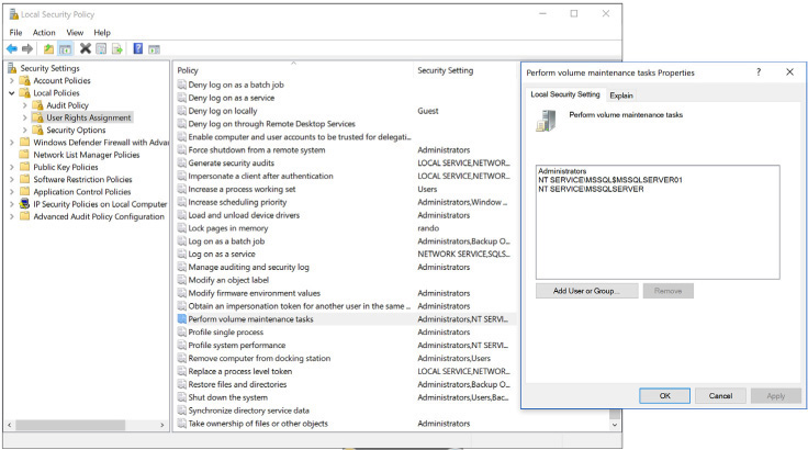
With instant file initialization, which is an Active Directory policy (Perform volume maintenance tasks), data files can be instantly resized, without zeroing-out the underlying file. This adds a major performance boost.

The trade-off is a tiny, perhaps insignificant security risk: data that was previously used in drive allocation currently dedicated to a database’s data file now might not have been fully erased before use. Because you can examine the underlying bytes in data pages using built-in tools in SQL Server, individual pages of data that have not yet been overwritten inside the new allocation could be visible to a malicious administrator.

Because this is a possible security risk, the Perform Volume Maintenance Tasks policy is not granted to the SQL Server service by default, and a summary of this warning is displayed during SQL Server setup.

Even so, turning on instant file initialization was a common post-installation step taken for many SQL Servers by DBAs, so this administrator-friendly option in SQL Server Setup is a welcome and recommended time-saving addition.

Without instant file initialization, you might find that the SQL Server wait type PREEMPTIVE_OS_WRITEFILEGATHER is prevalent during times of data-file growth. This wait type occurs when a file is being zero initialized; thus, it can be a sign that your SQL Server is wasting time that could skipped with the benefit of instant file initialization. Keep in mind that PREEMPTIVE_OS_WRITEFILEGATHER will also be generated by transaction log files, which cannot benefit from instant file initialization.

Note that SQL Server Setup takes a slightly different approach to granting this privilege than SQL Server administrators might take. SQL Server assigns Access Control Lists (ACLs) to automatically created security groups, not to the service accounts that you select on the Server Configuration Setup page. Instead of granting the privilege to the named SQL Server service account directly, SQL Server grants the privilege to the per-service security identifier (SID) for the SQL Server database service; for example, the NT SERVICEMSSQLSERVER principal. This means that the SQL Server service will maintain the ability to use instant file initialization even if its service account changes.

If you choose not to select the Perform Volume Maintenance Tasks privilege during SQL Server setup but want to do so later, go to the Windows Start menu, and then, in the Search box, type Local Security Policy. Next, in the pane on the left expand Local Policies (see Figure 3-6), and then click User Rights Assignment. Find the Perform Volume Maintenance Tasks policy, and then add the SQL Server service account to the list of objects with that privilege.

You can easily check to determine whether the SQL Server Database Engine service has been granted access to instant file initialization by using the sys.dm_server_services dynamic management view via the following query:

Click here to view code image

SELECT servicename, instant_file_initialization_enabled
FROM sys.dm_server_services
WHERE filename LIKE '%sqlservr.exe%';

Depending on the type of storage, the default allocation unit on NTFS might be 512 bytes, 4,096 bytes (also known as Advanced Format 4K sector size), or some other multiple of 512.

Because SQL Server deals with 64-KB extents (see the section “Mixed extents and uniform extents” earlier in the chapter), it makes sense to format a data volume with an allocation unit size of 64 KB, to align the extents with the allocation units.

• Windows Server. The Resilient File System (ReFS) was introduced with Windows Server 2012. It has seen significant updates since then, most recently in Windows Server 2016.

• Linux. SQL Server on Linux is supported on both the XFS and ext4 file systems. For ext4, the typical block size is 4 KB, though blocks can be created up to 64 KB. For XFS, the block size can range from 512 bytes to 64 KB.

Azure offers several ways to consider the management and querying of data in a SQL Server or SQL Server-like environment.

This section is divided into three main areas:

• Infrastructure as a service. SQL Server running on an Azure Virtual Machine.

• Platform as a service. Azure SQL Database and Azure SQL Data Warehouse (database as a service).

• Hybrid cloud. Combines the best features of on-premises SQL Server with Azure.

As we detail in Chapter 2, a VM shares physical resources with other VMs. In the case of Azure Virtual Machines, there are some configurations and optimizations that can make your SQL Server implementation perform well, without requiring insight into the other guest VMs.

When creating a SQL Server VM in Azure, you can choose from different templates, which provide a wide range of options for different virtual hardware configurations, OS, and, of course, version and edition of SQL Server.

Azure VMs are priced according to a time-based usage model, which makes it easier to get started. You pay per minute or per hour, depending on the resources you need, so you can start small and scale upward. In many cases, if performance is not acceptable, moving to better virtual hardware is very easy and requires only a few minutes of downtime.

Fortunately, some of these tasks have been done for you. For instance, power-saving settings are set to High Performance already, and TempDB files are configured properly when you configure a new Azure VM running SQL Server 2016 or higher.

However, Azure VMs have a limited selection for storage. You don’t have the luxury of custom Direct-Attached Storage or Storage-Area Networks dedicated to your environment. Instead, you can choose from the following options:

• Standard or Premium Storage

• Unmanaged or Managed Disks

• SQL Server data files in Microsoft Azure

• Standard Storage. Designed for low-cost, latency-insensitive workloads (https://docs.microsoft.com/azure/storage/common/storage-standard-storage).

• Premium Storage. Backed by solid-state drives. This is designed for use by low-latency workloads such as SQL Server.

Given our previously stated guidance to use the fastest drive possible, SQL Server is going to make better use of Premium Storage, because SQL Server’s main performance bottleneck is TempDB, followed closely by transaction log files, all of which are drive-bound.

It is possible to choose between unmanaged and managed disks:

• Unmanaged disks. VHDs are managed by you, from creating the storage account and the container, to attaching these VHDs to a VM and configuring any redundancy and scalability.

• Managed disks. You specify the size and type of drive you need (Premium or Standard), and Azure handles creation, management, and scalability for you.

Unmanaged disks give you more control over the drive, whereas managed disks are handled automatically, including resiliency and redundancy. Naturally, managed disks have a higher cost associated with them, but this comes with peace of mind.

As of this writing, there are several sizes to choose for Premium Storage, with more offerings being added all the time. Table 3-1 lists these offerings.

Maximum throughput can be limited by Azure VM bandwidth.

Microsoft recommends a minimum of two P30 drives for SQL Server data files. The first drive is for transaction logs, and the second is for data files and TempDB.

An important consideration with RAID is the stripe (or block) size. A 64-KB block size is most appropriate for an OLTP SQL Server environment, as noted previously. However, large data warehousing systems can benefit from a 256-KB stripe size, due to the larger sequential reads from that type of workload.

To read more about the different types of RAID, see Chapter 2.

For Azure VMs running SQL Server, if the storage account is located in the same location as the VM, there is no additional bandwidth cost.

To read more about using Azure Blob Storage with SQL Server, go to https://docs.microsoft.com/sql/relational-databases/tutorial-use-azure-blob-storage-service-with-sql-server-2016.

However, if there is any external access on the data, such as log shipping to a different location or using the AzCopy tool to synchronize data to another location (for example), there is a cost associated with that.

For more information about AzCopy, go to Microsoft Docs at https://docs.microsoft.com/azure/storage/common/storage-use-azcopy.

For drives hosting transaction logs, do not turn on caching.

You can read more about drive caching at https://docs.microsoft.com/azure/virtual-machines/windows/sql/virtual-machines-windows-sql-performance.

To get this to work, you need a storage account and container on Azure Storage, a Shared Access Signature, and a SQL Server Credential for each container.

Because performance is critical, especially when accessing storage over a network, you will need to test this offering, especially for heavy workloads.

There are some limitations that might affect your decision:

• FILESTREAM data is not supported, which affects memory-optimized objects, as well. If you want to make use of FILESTREAM or memory-optimized objects, you will need to use locally attached storage.

• Only .mdf, .ndf, and .ldf extensions are supported.

• Geo-replication is not supported.

You can read more (including additional limitations) at https://docs.microsoft.com/sql/relational-databases/databases/sql-server-data-files-in-microsoft-azure.

You can read more about performance best practices for SQL Server in Azure Virtual Machines at https://docs.microsoft.com/azure/virtual-machines/windows/sql/virtual-machines-windows-sql-performance.

It is possible to resize your VM within the same series (going larger is as simple as choosing a bigger size in the Azure portal), and in many cases, you can even move across series, as the need arises.

You can also downgrade your VM to a smaller size, to scale down after running a resource-intensive process, or if you accidentally overprovisioned your server. Provided that the smaller VM can handle any additional options you might have selected (data drives and network interfaces tend to be the deciding factor here), it is equally simple to downgrade a VM to a smaller size by choosing the VM in the Azure portal.

Both growing and shrinking the VM size does require downtime, but it usually takes just a few minutes at most.

To quote directly from Microsoft Docs:

“Dv2-series, D-series, G-series, are ideal for applications that demand faster CPUs, better local disk performance, or have higher memory demands. They offer a powerful combination for many enterprise-grade applications.” (https://docs.microsoft.com/azure/cloud-services/cloud-services-sizes-specs)

This makes the D-series (including Dv2 and Dv3) and G-series well suited for a SQL Server VM.

However, choosing the right series can be confusing, especially with new sizes and series coming out all the time. The ability to resize VMs makes this decision less stressful.

A fairly common practice with Azure VMs is to place the SQL Server TempDB on this temporary drive because it uses solid-state storage and is theoretically faster than a Standard Storage drive.

However, this temporary drive is thinly provisioned. Remember in Chapter 2 how thin provisioned storage for VMs is shared among all the VMs on that host.

Placing the TempDB on this drive is risky, because it can result in high latency, especially if other guests using that underlying physical storage have done the same thing. This is also affected by the series of VM.

To keep things simple, place TempDB on its own dedicated Premium Storage drive (if the VM supports it) or at least sharing a larger Premium Storage drive with other databases. For example, a P30 drive is 1,024 MB in size, and provides 5,000 IOPS.

You can use database as a service (DBaaS), which includes Azure SQL Database and Azure SQL Data Warehouse, to complement or replace your organization’s data platform requirements. This section focuses on Azure SQL Database.

Azure SQL Database provides you with a single database (or set of databases logically grouped in an elastic pool) and the freedom not to concern yourself with resource allocation (CPU, RAM, storage, licensing, OS), installation, and configuration of that database.

You also don’t need to worry about patching and upgrades at the OS or instance level, nor do you need to think about index and statistics maintenance, TempDB, backups, corruption, or redundancy. In fact, the built-in support for database recovery is excellent (including point-in-time restores), so you can even add on long-term backup retention to keep your backups for up to 10 years.

Microsoft’s Data Platform is about choosing the right component to solve a particular problem, as opposed to being all things to all people.

Azure SQL Database and Azure SQL Data Warehouse are part of a larger vision, taking the strengths of the database engine and combining them with other Azure components, breaking the mold of a self-contained or standalone system. The change in mindset is necessary to appreciate it for what it offers, instead of criticizing it for its perceived shortcomings.

Think of Azure SQL Database, then, as an offering at the database level. Because of this, only database-specific features are available. You can create objects such as tables, views, user-defined functions, and stored procedures, as well as memory-optimized objects. You can write queries. And, you can connect an application to it.

What you can’t do with Azure SQL Database is run scheduled tasks directly. Querying other databases is extremely limited. You can’t restore databases from a SQL Server backup. You don’t have access to a file system, so importing data is more complicated. You can’t manage system databases, and in particular, you can’t manage TempDB.

There is currently no support for user-defined SQL Server CLR procedures. However, the native SQL CLR functions, such as those necessary to support the hierarchyid and geospatial data types, are available.

On-premises environments usually use only Integrated Authentication to provide single sign-on and simplified login administration. In such environments, SQL authentication is often turned off. Turning off SQL authentication is not supported in Azure SQL Database. Instead of Integrated Authentication, there are several Azure Active Directory authentication scenarios supported. Those are discussed in more detail in Chapter 5, “Provisioning Azure SQL Database.”

Azure SQL Database does not support multiple filegroups or files. By extension, several other Database Engine features that use filegroups are unavailable, including FILESTREAM and FileTable.

You can read more about FILESTREAM and FileTable in Chapter 8.

Most important, Azure SQL databases are limited by physical size, and resource usage.

The resource limits, known as Database Transaction Units (DTUs), force us to rethink how we make the best use of the service. It is easy to spend a lot of wasted money on Azure SQL Database because it requires a certain DTU service level at certain periods during the day or week, but at other times is idle.

It is possible to scale an Azure SQL database up and down as needed, but if this happens regularly, it makes the usage, and therefore the cost, unpredictable. Elastic pools (see the upcoming section on this) are a great way to get around this problem by averaging out DTU usage over multiple databases with elastic DTUs (eDTUs). That said, Azure SQL Database is not going to completely replace SQL Server. Some systems are not designed to be moved into this type of environment, and there’s nothing wrong with that. Microsoft will continue to release a standalone SQL Server product.

On the other hand, Azure SQL Database is perfect for supporting web applications that can scale up as the user base grows. For new development, you can enjoy all the benefits of not having to maintain a database server, at a predictable cost.

Just as with choosing between SQL Server 2017 editions, selecting the right service tier is important. The Basic and Standard service tiers do not support Columnstore or memory-optimized objects. The Basic tier provides only seven days of backups versus 35 days on the higher tiers. Premium and Premium RS have a much lower I/O latency than Standard tier.

However, it is fairly easy to switch between service tiers on Azure SQL Database, especially between the different levels in each tier, and when combined with elastic pools, this gives you great flexibility and predictable usage costs.

Finally, Microsoft operates under a cloud-first strategy, meaning that features will appear in Azure SQL Database before they make it to the latest on-premises products. Given the length of time it takes for many organizations to upgrade, the benefits are even more immediate and clear.

Elastic pools increase the scalability and efficiency of your Azure SQL Database deployment by providing the ability for several databases in a pool to share DTUs. In that case, the combined DTUs are referred to as elastic DTUs (eDTUs).

Without using elastic pools, each database might be provisioned with enough DTUs to handle its peak load. This can be inefficient. By grouping databases with different peak load times in an elastic pool, the Azure fabric will automatically balance the DTUs assigned to each database depending on their load, as depicted in Figure 3-7. You can set limits to ensure that a single database does not starve the other databases in the pool of resources.

The best use case for elastic pools is one in which databases in the pool have low average DTU utilization, with spikes that occur from time to time. This might be due to a reporting-type query that runs once a day, or a help desk system that can experience a lot of traffic at certain times of the day, for instance.

The elastic pool evens out these spikes over the full billing period, giving you a more predictable cost for an unpredictable workload across multiple databases.

Multitenant architecture Azure SQL databases in an elastic database pool gives you the ability to provision new databases for your customer base with predictable growth and associated costs. Management of these databases is much easier in this environment because the administrative burden is removed. Performance is also predictable because the pool is based on the combined eDTUs.

However, not all scenarios will benefit from the use of elastic pools. The most beneficial are those in which databases experience their peak load at separate times. You would need to monitor the usage patterns of each customer and plan which elastic database pool they work best in, accordingly.

Database consolidation In an on-premises environment, database consolidation means finding a powerful enough server to handle the workload of many databases, each with its own workload pattern. Similarly, with elastic database pools, the number of databases is limited by the pool’s eDTU size. For example, the current maximum pool size is 4,000 eDTUs in a Premium pool. This means that you can operate up to 160 databases (at 25 DTUs each) in that single pool, sharing their resources.

Combined with autoscale settings, depending on DTU boundaries, consolidation makes a lot of sense for an organization with many small databases, just as it does with an on-premises SQL Server instance.

As a workaround, you can place the databases that you want to combine in a logical group inside an elastic database pool. This makes it possible for you to perform cross-database queries on them as well as to connect to external data in the form of Microsoft Excel, Microsoft Power BI, and so on.

There are some limitations. As of this writing, elastic database query is still in preview. On the Standard tier, the first query can take several minutes to run because the functionality to run the query needs to be loaded first. Additionally, access is currently read-only for external data.

Performance does improve on the higher tiers as costs increase, but this is not meant to replicate home-grown systems that have many databases tightly bound together.

Because this makes use of other Azure services, including Azure Cloud Service and Azure Service Bus, there is an additional cost associated with elastic database jobs because of the way the platform is designed.

For example, in a software as a service (SaaS) scenario in which each customer receives its own database instance, the schemas of all databases must be kept synchronized. An elastic pool job can target the databases that are part of a custom group of databases. A job is inserted into a control database (a standalone Azure SQL database). The controller (one of two worker roles created with the Cloud Service) then reads the job, and a second worker role runs that job task against each database in the pool using an activator (making use of the Azure Service Bus component). Finally, the results are stored in the control database, and diagnostics are saved to an Azure Storage container.

You can read about Elastic Scale in Chapter 5, and find out more about elastic database jobs, such as their architecture and setup, at https://docs.microsoft.com/azure/sql-database/sql-database-elastic-jobs-overview.

Sharding is a technique by which data is partitioned horizontally across multiple nodes, either to improve performance or the resiliency of an application. In the context of Azure SQL Database, sharding refers to distributing data across more than one database when it grows too large. (If this sounds like table partitioning, you’re mostly right.)

It is all very well to add more databases (shards) to support your application, but how do you distribute your data evenly across those new databases?

The Split-Merge tool can move data from constrained databases to new ones while maintaining data integrity. It runs as an Azure web service, which means there is an associated cost. The tool uses shard map management to decide what data segments (shardlets) go into which database (shard) using a metadata store (an additional standalone Azure SQL Database) and is completely customizable.

To read about how this process works in detail, go to https://docs.microsoft.com/azure/sql-database/sql-database-elastic-scale-overview-split-and-merge.

The most common implementation of a hybrid cloud is with Azure Active Directory (Azure AD). Instead of having to manage user accounts in two places (on-premises and in Azure, for Microsoft Office 365, for example), you can synchronize your Active Directory Domain Service with Azure AD, and manage it all in one place.

Mixing your on-premises and Azure environments, in whichever way you do it, falls under the definition of a hybrid cloud, and Microsoft has some interesting ways of helping you achieve this, especially around the data platform and SQL Server.

Stretch Database is designed to balance the needs of keeping cold data online, by reducing the cost of storing and managing that data locally and reducing RTO and RPO mandated in a Service-Level Agreement (SLA).

Because historic data can account for a large percentage of an existing database, removing cold data from an on-premises database can significantly reduce the storage, time, and other resources for necessary tasks like backups, index and statistics maintenance, data consistency checks, and so on, while still making it available to be queried.

Stretch Database is activated at the instance level, but you move rows at a database and table level. If your cold data is already stored in a separate archive table, you can move the entire table. If your cold data is in a large table that also contains active, or hot data, you can set up a filter to move only the older rows.

No application changes are needed, but there are some considerable limitations to using Stretch Database:

• Constraints in the migrated data are not enforced for uniqueness (including primary key and unique constraints), and you cannot move tables containing foreign keys and check constraints.

• You cannot perform any data modification on migrated data (updates and deletes), and you cannot insert rows directly (they must be moved in by the Stretch Database functionality).

• You cannot perform data modification on the data that is eligible for migration.

• You cannot create indexes on views that refer to Stretch-configured tables, and you cannot move tables that are used in existing indexed views.

• Filters on indexes are not propagated on migrated data, which can cause issues with unique filtered indexes.

There are also limits to the type of data and indexes that can participate in a Stretch Database:

• text, ntext, and image data types are not permitted.

• timestamp (rowversion), xml, and sql_variant types are not permitted.

• CLR (Common Language Runtime, or .NET) data types are not permitted (including geography, geometry, and hierarchyid).

• Computed columns are not permitted.

• Full-text, XML, and spatial indexes are not permitted.

Finally, the costs for Stretch Database are based on both storage and compute models. This means that you will pay for storage even if you never query the data. If you query the data, you will also pay for the compute costs (priced according to a Database Stretch Unit, or DSU) as well as any data transfer.

These limitations might exist for good reasons, but those reasons could be enough cause to consider alternatives. However, for ease of use, Stretch Database works as advertised.

By default, the schedule depends on the transaction workload, so a server that is idle will have fewer transaction log backups than a busy server. This reduces the total number of backup files required to restore a SQL Server database in a disaster recovery (DR) scenario.

You can also use advanced options to define a schedule. However, you must set this up before turning on Managed Backups to avoid unwanted backup operations. Additionally, the retention period is customizable, with the maximum being 30 days.

You can configure these backups at the instance or database level, providing much needed flexibility for smaller database environments that would not ordinarily have a full-time database administrator on hand.

You can fully encrypt backups through SQL Server backup encryption, and Azure Blob Storage is encrypted by default (for data at rest).

You can read more about encryption in Chapter 7.

There is an associated cost with the Azure Storage container required to store these database backups, but when the retention period is reached, older files will be cleared out, keeping the costs consistent. If you were building your own custom backup solution, you would incur similar costs anyway, and there is a good chance the managed backup storage costs will be lower.

To read more about SQL Server Managed Backup to Microsoft Azure, go to https://docs.microsoft.com/sql/relational-databases/backup-restore/sql-server-managed-backup-to-microsoft-azure.

After you have developed the solutions that best suit your organization, you can deploy your applications and solutions to the Azure region that makes the most sense, or just keep them on-premises, hosted on Azure Stack.

You can expose Azure SQL databases as a service by using the SQL Server resource provider. This gives your users the ability to create databases without having to provision a VM every time. Think of it as an on-premises version of Azure SQL Database.

Keep in mind that certain features like elastic pools, and scaling databases, are not available at this time.

You can read more about Azure SQL databases on Azure Stack at https://docs.microsoft.com/azure/azure-stack/azure-stack-sql-resource-provider-deploy.

Many organizations want to ensure a secure channel between their environments, be it between Azure VNets, or between their on-premises network and Azure. You can achieve this by way of a Virtual Private Network (VPN).

A VPN encrypts traffic over any network (including the internet), through a tunnel it creates. All traffic that travels through that tunnel is secure, which means that no bad actors will be able to monitor the traffic. However, there is a performance overhead with encrypting that traffic, which makes the connection slightly slower.

There are two main ways that Azure implements connections between your on-premises environment and Azure itself. One of these is through a traditional VPN service over the internet (site-to-site), and the other is through a dedicated connection that does not use the public internet (Azure ExpressRoute).

Site-to-site VPN There are two different types of problems that you need to deal with when connecting systems to an Azure VNet: connecting two Azure VNets together, and connecting an external network to an Azure VNet.

To connect two Azure VNets together in the same region, you can create a peering network—in other words, no part of the VNet goes out to the internet, which is priced (very reasonably) per gigabyte transferred.

If you want a VPN gateway, instead, which creates a connection between your on-premises network and an Azure VNet, those are priced according to the maximum bandwidth you would require (100 Mbps, 500 Mbps, 1 Gbps, and 1.25 Gbps), and charged at an hourly rate (which, depending on what you need, is also reasonably priced).

Azure ExpressRoute If those speeds are not satisfactory, and you want to connect your on-premises network to your Azure VNet, you can use ExpressRoute.

With its low latency, ExpressRoute expands your existing network to the virtually limitless services available in Azure, depending on your budget, of course.

According to Microsoft Docs:

ExpressRoute is “…excellent for scenarios like periodic data migration, replication for business continuity, disaster recovery, and other high-availability strategies.” (https://azure.microsoft.com/services/expressroute)

This type of bandwidth gives you the flexibility of moving entire VMs from on-premises to Azure, for test environments and migrations. Your customers can use Azure web services that take data from your on-premises environment without ever going over the public internet.

You can also use it for creating a DR site, using SQL Server Log Shipping. Perhaps you want to extend your availability group to the cloud, which you can do by using a distributed availability group (see Chapter 2). Using ExpressRoute, you can treat Azure as an extension of your own network, as illustrated in Figure 3-8.