
In the previous chapters, we spent significant time on how we can query data stored inside SQL Server instances or on HDFS through Spark. One advantage of having access to data stored in different formats is that it allows you to perform analysis of the data at a large, and distributed, scale. One of the more powerful options we can utilize inside Big Data Clusters is the ability to implement machine learning solutions on our data. Because Big Data Clusters allow us to store massive amounts of data in all kinds of formats and sizes, the ability to train, and utilize, machine learning models across all of that data becomes far easier.
In many situations where you are working with machine learning, the challenge to get all the data you need to build your models on in one place takes up the bulk of the work. Building a machine learning model (or training as it is called in the data science world) becomes far easier if you can directly access all the data you require without having to move it from different data sources to one place. Besides having access to the data from a single point of entry, Big Data Clusters also allow you to operationalize your machine learning models at the same location where your data resides. This means that, technically, you can use your machine learning models to score new data as it is stored inside your Big Data Cluster. This greatly increases the capabilities of implementing machine learning inside your organization since Big Data Clusters allow you to train, exploit, and store machine learning models inside a single solution instead of having various platforms in place to perform a specific action inside your organization’s advanced analytics platform.
In this chapter we are going to take a closer look at the various options available inside Big Data Clusters to train, store, and operationalize machine learning models. Generally speaking, there are two directions we are going to cover: In-Database Machine Learning Services inside SQL Server and machine learning on top of the Spark platform. Both of these areas cover different use cases, but they can also overlap. As you have seen in the previous chapter, we can easily bring data stored inside a SQL Server instance to Spark and vice versa if we so please. The choice of which area you choose to perform your machine learning processes on is, in this situation, more based on what solution you personally prefer to work in. We will discuss the various technical advantages and disadvantages of both machine learning surfaces inside Big Data Clusters in each section of this chapter. This will give you a better understanding of how each of these solutions works and hopefully will help you select which one fits your requirements the best.
SQL Server In-Database Machine Learning Services
With the release of SQL Server 2016, Microsoft introduced a new feature named in-database R Services. This new feature allows you to execute R programming code directly inside SQL Server queries using either the new sp_execute_external_script stored procedure or the sp_rxPredict CLR procedure. The introduction of in-database R Services was a new direction that allowed organizations to integrate their machine learning models directly inside their SQL Server databases by allowing the user to train, score, and store models directly inside SQL Server. While R was the only language available inside SQL Server 2016 for use with sp_execute_external_script , Python was added with the release of SQL Server 2017 which also resulted in a rename of the feature to Machine Learning Services. With the release of SQL Server 2019, on which Big Data Clusters are built, Java was also added as the third programming language that is available to access directly from T-SQL code.
While there are some restrictions in place regarding In-Database Machine Learning Services (for instance, some functions that are available with In-Database Machine Learning Services, like PREDICT , only accept algorithms developed by Revolution Analytics machine learning models), it is a very useful feature if you want to train and score your machine learning models very closely to where your data is stored. This is also the area where we believe In-Database Machine Learning Services shine. By utilizing the feature data movement is practically minimal (considering that the data your machine learning models require is also directly available in the SQL Server instance), model management is taken care of by storing the models inside SQL Server tables, and it opens the door for (near) real-time model scoring by passing the data to your machine learning model before it is stored inside a table in your database.
All of the example code inside this chapter is available as a T-SQL notebook at this book’s GitHub page. For the examples in this section, we have chosen to use R as the language of choice instead of Python which we used in the previous chapter.
Training Machine Learning Models in the SQL Server Master Instance
Before we can get started training our machine learning models, we have to enable the option to allow the use of the sp_execute_external_script function inside the SQL Server Master Instance of the Big Data Cluster. If you do not enable the option to run external scripts inside the SQL Instance, a large portion of the functionality of In-Database Machine Learning Services is disabled.
Some In-Database Machine Learning functionality is still with external scripts disabled. For instance, you can still use the PREDICT function together with a pretrained machine learning model to score data. However, you cannot run the code needed to train the model, since that mostly happens through the external script functionality.

Error running sp_execute_external_script with external scripts disabled
Enable external scripts
Sample R code using sp_execute_external_script
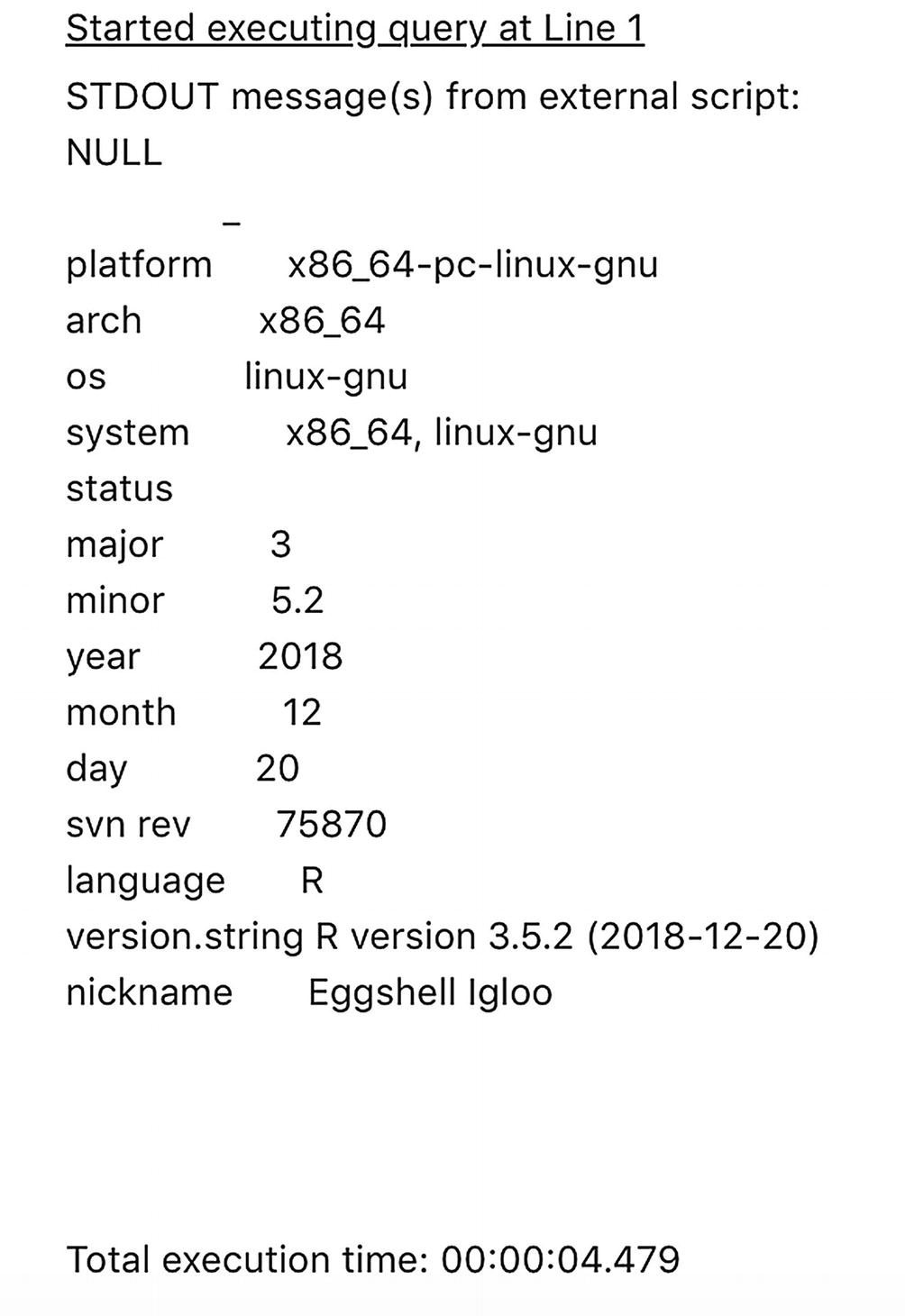
R version results through sp_execute_external_script
As you can see from the code, the sp_execute_external_script procedure accepts a number of parameters. Our example displays the minimal parameters that need to be supplied when calling the procedure, namely, @language and @script. The @language parameter sets the language that is used in the @script section. In our case, this is R. Through the @script parameter, we can run the R code we want to execute, in this case the print (version) command.
While sp_execute_external_script always returns results regarding the machine it is executed on, the output of the print (version) R command starts on line 5 with _ platform x86_64.
Returning data using WITH RESULT SETS
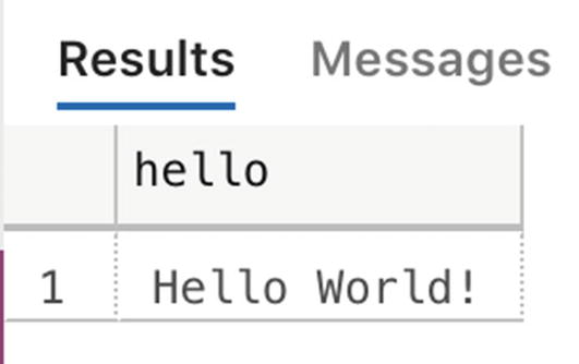
Output returned to a table format
Just like how we can define and map output results through the sp_execute_external_script procedure , we can define input datasets. This is of course incredibly useful since this allows us to define a query as an input dataset to the R session and map it to an R variable. Being able to get data stored inside your SQL Server database inside the In-Database Machine Learning Service feature opens up the door to perform advanced analytics on that data like training or score machine learning models.
We are going to train a machine learning model on the “Iris” dataset. This dataset is directly available inside R and shows various characteristics of Iris flowers and to which species a specific Iris flower belongs. We can use this data to create a classification machine learning model in which we are going to predict which species an Iris flower belongs to.
Create a new database and fill it with test data
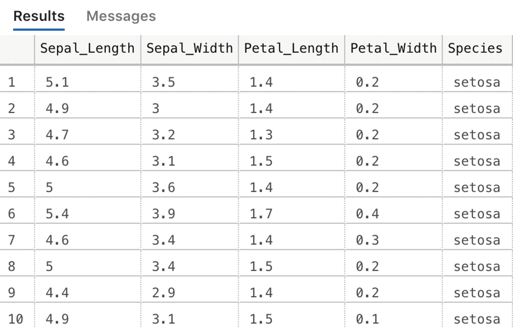
Iris table values
Create model table
Next to the model_object column that is going to hold our serialized model, we also create two additional columns that store the name and the version of the model. This can be very useful in situation where you are storing multiple models inside your SQL Server database and want to select a specific model version or name.
The next thing we are going to do is to split our Iris dataset into a training and a testing set. Splitting a dataset is a common task when you are training machine learning models. The training dataset is the data you are going to use to feed into the model you are training; the test dataset is a portion of the data you are “hiding” from the model while it is training. In that way the model was never exposed to the testing data, which means we can use the data inside the testing set to validate how well the model performs when shown data is has never seen before. For that reason, it is very important that both the training and the testing datasets are a good representation of the full dataset. For instance, if we train the model only on characteristics of the “Setosa” Iris species inside our dataset and then show it data from another species through our test dataset, it will predict wrong (predicting Setosa) since it has never seen that other species during training.
Split dataset into training and testing dataset
Train a machine learning model using sp_execute_external_script
- 1.
The first line of the script, DECLARE @model VARBINARY(MAX), declares a T-SQL variable of the VARBINARY datatype that will hold our model after training it.
- 2.
In the second step, we execute the sp_execute_external_script procedure and supply the R code needed to train our model. Notice we are using an algorithm called rxDTree. rxDTree is a decision tree algorithm building by Revolution Analytics, a company that Microsoft bought in 2015 and provided parallel and chunk-based algorithms for machine learning. The syntax for the model training is pretty straightforward; we are predicting the species based on the other columns (or as they are called: features) of the training dataset.
The line trained_model <- rxSerializeModel(iris.dtree, realtimeScoringOnly = FALSE) is the command to serialize our model and store inside the trained_model R variable. We map that variable as an output parameter to the T-SQL @model variable in the call to the sp_execute_external_script procedure. We map the query that selects all the records from the training dataset as an input variable for R to use as input for the algorithm.
- 3.
Finally, in the last step, we insert the trained model inside the model table we created earlier. We supply some additional data like a name and a version so we can easily select this model when we use it to predict Iris species in the next step.

Trained decision tree model inside the model table
Scoring Data Using In-Database Machine Learning Models
Now that we have trained our model, we can use it to score, or predict, the data we stored in the Iris_test table. To do that we can use two methods, one using the sp_execute_external_script procedure which we have also used to train our model and the other by using the PREDICT function that is available in SQL Server.
Run a prediction using the in-database stored model
In the first part of the R script inside the sp_execute_external_script code, we have to unserialize our model again using rxUnserializeModel. With the model unserialized, we can perform a prediction of the input data. The last line of R code adds the probability columns for each Iris species to the input dataset. This means we end up with a single table as output that contains all the input columns as well as the columns generated by the scoring process.
We won’t go into details about machine learning or machine learning algorithms in this book, but the problem we are trying to solve using machine learning in this case is one called classification. Machine learning algorithms can basically be grouped into three different categories: regression, classification, and clustering. With regression we are trying to predict a numerical value, for instance, the price of a car. Classification usually deals with predicting a categorical value, like the example we went through in this chapter: What species of Iris plant is this? Clustering algorithms try to predict a result by trying to group categories together based on their characteristics. In the Iris example we could also have chosen to use a clustering algorithm since there might be clear Iris species characteristics that tend to group together based on the species.
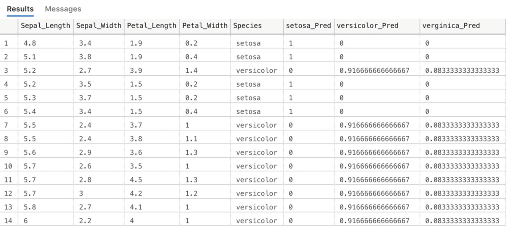
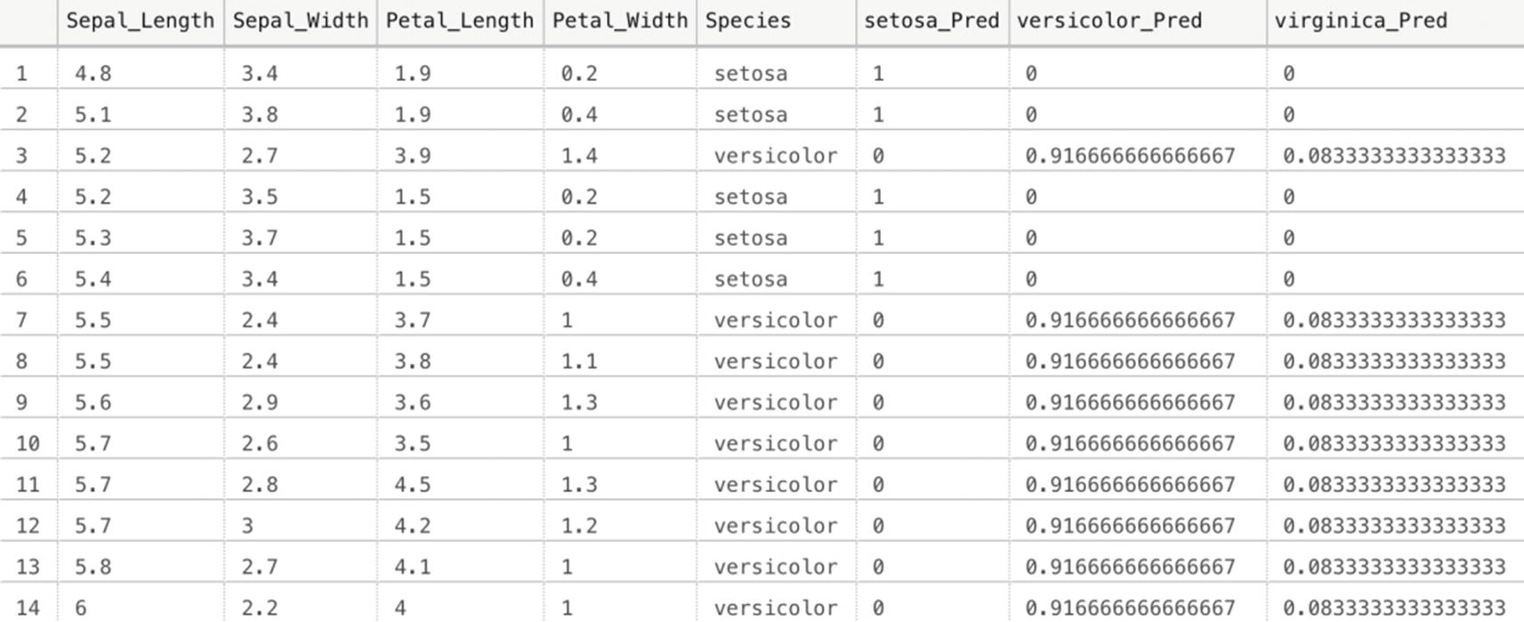
Scored results for the data inside the Iris_test table using our trained machine learning model
Performing a prediction using the sp_execute_external_script method works perfectly fine and gives you maximum flexibility in terms of what you can do using R code. However, it does result in quite a lot of lines of code. Another method we have available inside SQL Server is using the PREDICT function; PREDICT is far easier to use, has a simpler syntax, and, in general, performs faster than sp_execute_external_script. It does have its drawbacks though, for instance, you cannot write custom R code to perform additional steps on the data and you are required to use a serialized model that was trained using a Revolution Analytics algorithm (by using sp_execute_external_script you can basically use every algorithm available in R or R libraries).
Running a model prediction using the PREDICT function
Iris species prediction using PREDICT
Now that we have trained a machine learning model, and scored data using it, inside SQL Server Machine Learning Services, you should have a general idea of the capabilities of these methods. In general, we believe In-Database Machine Learning Services is especially useful when all, or the largest part, of your data is stored inside SQL Server databases. With the model stored inside a SQL Server database as well, you can build solutions that are able to (near) real-time score data as soon as it is stored inside your SQL Server database (for instance, by using triggers that call the PREDICT function). If you want to, you are not limited to just SQL Server tables however. As you have seen in earlier chapters, we can map data stored inside the Spark cluster (or on other systems all together) using external tables and pass that data to the In-Database Machine Learning Services.
In some situations, however, you cannot use In-Database Machine Learning Services, perhaps because your data doesn’t fit inside SQL Server, either by size or by data type, or you are more familiar with working on Spark. In any of those cases, we always have the option of performing machine learning tasks on the Spark portion of the Big Data Cluster which we are going to explore in more detail in the next section.
Machine Learning in Spark
Since Big Data Clusters are made up from SQL Server and Spark nodes, we can easily choose to run our machine learning processes, from training to scoring, inside the Spark platform. There are many reasons we can come up with why you would choose Spark over SQL for a machine learning platform (and vice versa). However, when you have a very large dataset that doesn’t make sense to load into a database, you are more or less stuck on using Spark since Spark can handle large datasets very well and can train various machine learning algorithms in the same distributed nature as it handles data processing.
As expected on an open, distributed, data processing platform, there are many libraries available which you can use to satisfy your machine learning needs. In this book we decided on using the built-in Spark ML libraries which provide a large selection of different algorithms and should cover most of your advanced analytical needs.
Reading data from the SQL Server Master Instance
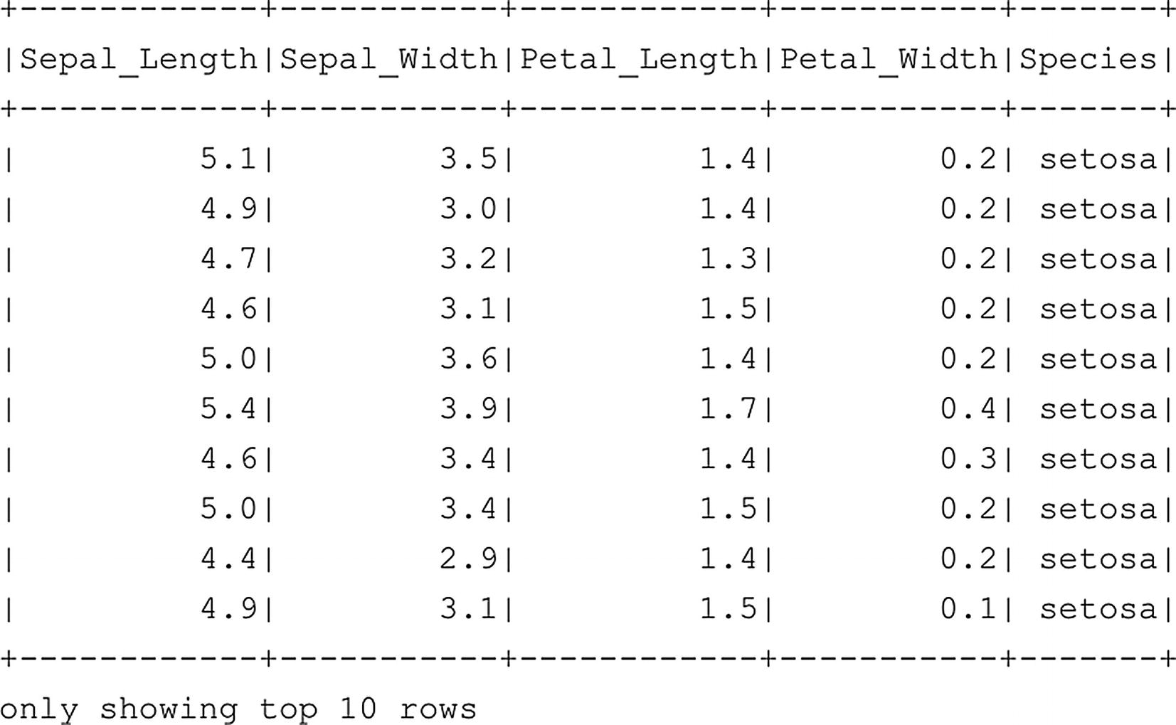
df_Iris dataframe top ten rows
Loading machine learning libraries
In this case, since we are doing a so-called classification problem, we only need to import the pyspark.ml.classification libraries together with the libraries we need to perform some modification to the features (which is another name for the columns of our dataframe in this case) of the dataframe and evaluate our model performance.
Process the data so it is suitable for machine learning
The first code section combines the different features inside a new column called “features.” All of these features are Iris species characteristics and they are combined into a single format called a vector (we will take a look at how this visually looks a bit further down in the book). The line feature_cols = df_Iris.columns[:-1] selects all the columns of the dataframe except the rightmost column which is the actual species of the Iris plant.
In the second section, we are mapping the different Iris species to a numerical value. The algorithm we are going to use to predict the Iris species requires numerical input, which means we have to perform a conversion. This is not unusual in the realm of machine learning and data science. In many cases you have to convert a string value to a numerical value so the algorithm can work with it. After the conversion from string to numerical, we add a new column called “label” which contains the species in a numerical value.
Only select the features and label dataframe columns
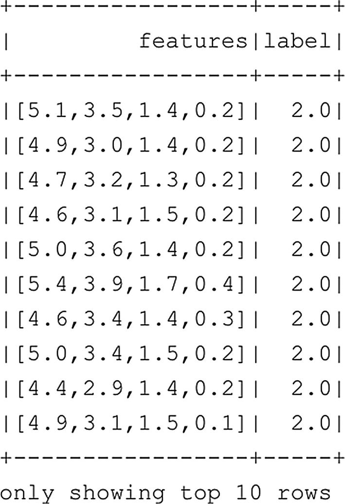
modified df_Iris dataframe
As you can see from Figure 7-9, all of the features (Petal_Length, Petal_Width, etc.) have been transformed inside a single vector inside a single column of our dataframe. The label column now returns a number for the species, 2.0 being Setosa, 1.0 virginica, and 0.0 versicolor.
Split the dataframe into a training and testing dataframe
Initiate the classifier
In this case we have chosen to use a logistic regression algorithm to try and predict which species of Iris a plant belongs to, based on its characteristics. We are going to ignore the algorithm parameters for now. When you are in the phase when you try to optimize and tune your model, you will frequently go back to the parameters (either manually or programmatically) and modify them to find the optimal setting.
Train the model
Perform a prediction
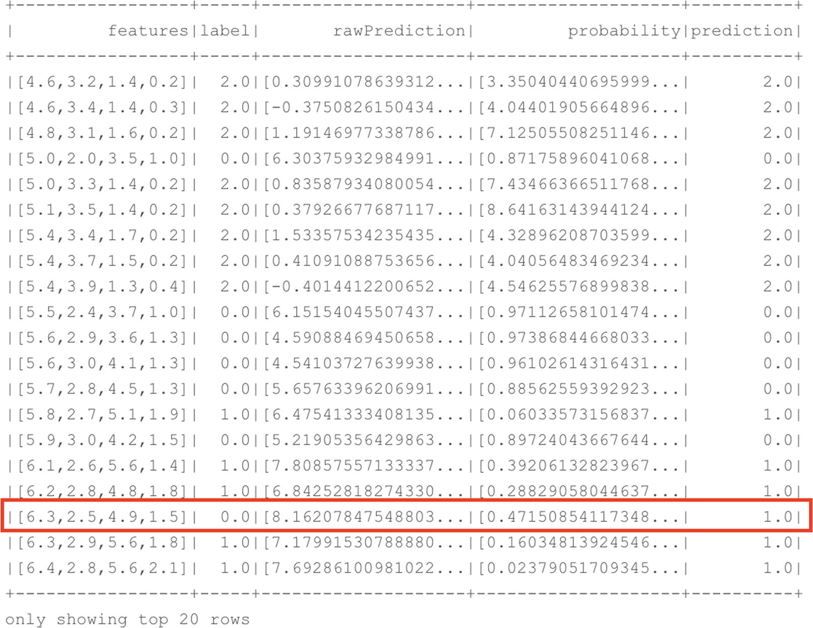
Prediction results on our test dataset
As you can see in Figure 7-10, our model performed a good job on the test dataset. In the top 20 rows that were returned by the command, only a single row had a prediction for a different species instead of the actual one (we predicted virginica while it should have been versicolor). While we could analyze each and every row to look for differences between the actual species and the predicted species, a far faster way to look at model performance is by using the Spark ML evaluation library which we loaded earlier.
Measuring model performance
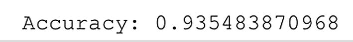
Accuracy of our trained model
With our model trained and tested, we can take additional steps depending on what we are planning to do with the model. If we are interested in optimizing model performance more, we could go back and tune our algorithm parameters before training the model again. Perhaps it would also be useful, in this scenario, to look how good the split is between the training and test dataset since that has a huge impact on the model accuracy and there are a hundred more things we could do to optimize our model even further if we wanted to (even selecting a different algorithm to see if that predicts better than the current one).
Another thing we could do is store the model. We are way more flexible in that area than inside SQL Server In-Database Machine Learning Services where the model had to be serialized and stored inside a table. In the case of Spark, we can choose different methods and libraries to store our models. For instance, we can use a library called Pickle to store our model on the filesystem, or use the .save function on the model variable to store it on an HDFS location of our choosing. Whenever we need our trained model to score new data, we can simply load it from the filesystem and use it to score the new data.
Summary
In this chapter we explored the various methods available to perform machine learning tasks inside SQL Server Big Data Clusters. We looked at SQL Server In-Database Machine Learning Services which allowed us to train, utilize, and store machine learning models directly inside the SQL Server Master Instance using a combination of T-SQL queries and the new sp_execute_external_script procedure. In the Spark department, we also have a wide variety of machine learning capabilities available to use. We used the Spark ML library to train a model on a dataframe and used it to score new data. Both of the methods have their strengths and weaknesses, but having both of these solutions available inside a single box allows optimal flexibility for all our machine learning needs.