Hour 17. Improving Database Performance
What You’ll Learn in This Hour:
• What SQL statement tuning is
• Database tuning versus SQL statement tuning
• Formatting your SQL statement
• Properly joining tables
• The most restrictive condition
• Full table scans
• Invoking the use of indexes
• Avoiding the use of OR and HAVING
• Avoiding large sort operations
In this hour, you learn how to tune your SQL statement for maximum performance using some simple methods.
What Is SQL Statement Tuning?
SQL statement tuning is the process of optimally building SQL statements to achieve results in the most effective and efficient manner. SQL tuning begins with the basic arrangement of the elements in a query. Simple formatting can play a rather large role in the optimization of a statement.
SQL statement tuning mainly involves tweaking a statement’s FROM and WHERE clauses. It is mostly from these two clauses that the database server decides how to evaluate a query. To this point, you have learned the FROM and WHERE clauses’ basics. Now it is time to learn how to fine-tune them for better results and happier users.
Database Tuning Versus SQL Statement Tuning
Before this hour continues with your SQL statement tuning lesson, you need to understand the difference between tuning a database and tuning the SQL statements that access the database.
Database tuning is the process of tuning the actual database, which encompasses the allocated memory, disk usage, CPU, I/O, and underlying database processes. Tuning a database also involves the management and manipulation of the database structure, such as the design and layout of tables and indexes. In addition, database tuning often involves the modification of the database architecture to optimize the use of the hardware resources available. You need to consider many other things when tuning a database, but the database administrator (DBA) in conjunction with a system administrator normally accomplishes these tasks. The objective of database tuning is to ensure that the database has been designed in a way that best accommodates expected activity within the database.
SQL tuning is the process of tuning the SQL statements that access the database. These SQL statements include database queries and transactional operations, such as inserts, updates, and deletes. The objective of SQL statement tuning is to formulate statements that most effectively access the database in its current state, taking advantage of database and system resources and indexes. The objective is to reduce the operational overhead of executing the query on the database.
By the Way: Tuning Is Not One Dimensional
You must perform both database tuning and SQL statement tuning to achieve optimal results when accessing the database. A poorly tuned database might render your efforts in SQL tuning as wasted, and vice versa. Ideally, it is best to first tune the database, ensure that indexes exist where needed, and then tune the SQL code.
Formatting Your SQL Statement
Formatting your SQL statement sounds like an obvious task, but it is worth mentioning. A newcomer to SQL will probably neglect to consider several things when building an SQL statement. The upcoming sections discuss the following considerations; some are common sense, others are not so obvious:
• The format of SQL statements for readability
• The order of tables in the FROM clause
• The placement of the most restrictive conditions in the WHERE clause
• The placement of join conditions in the WHERE clause
Formatting a Statement for Readability
Did You Know?: It’s All About the Optimizer
Most relational database implementations have what is called an SQL optimizer, which evaluates an SQL statement and determines the best method for executing the statement based on the way an SQL statement is written and the availability of indexes in the database. Not all optimizers are the same. Check your implementation or consult the database administrator to learn how the optimizer reads SQL code. You should understand how the optimizer works to effectively tune an SQL statement.
Formatting an SQL statement for readability is fairly obvious, but many SQL statements have not been written neatly. Although the neatness of a statement does not affect the actual performance (the database does not care how neat the statement appears), careful formatting is the first step in tuning a statement. When you look at an SQL statement with tuning intentions, making the statement readable is always the first priority. How can you determine whether the statement is written well if it is difficult to read?
Some basic rules for making a statement readable include
• Always begin a new line with each clause in the statement. For example, place the FROM clause on a separate line from the SELECT clause. Then place the WHERE clause on a separate line from the FROM clause, and so on.
• Use tabs or spaces for indentation when arguments of a clause in the statement exceed one line.
• Use tabs and spaces consistently.
• Use table aliases when multiple tables are used in the statement. The use of the full table name to qualify each column in the statement quickly clutters the statement and makes reading it difficult.
• Use remarks sparingly in SQL statements if they are available within your specific implementation. Remarks are great for documentation, but too many of them clutter a statement.
• Begin a new line with each column name in the SELECT clause if many columns are being selected.
• Begin a new line with each table name in the FROM clause if many tables are being used.
• Begin a new line with each condition of the WHERE clause. You can easily see all conditions of the statement and the order in which they are used.
The following is an example of a statement that would be hard for you to decipher:
SELECT CUSTOMER_TBL.CUST_ID, CUSTOMER_TBL.CUST_NAME,
CUSTOMER_TBL.CUST_PHONE, ORDERS_TBL.ORD_NUM, ORDERS_TBL.QTY
FROM CUSTOMER_TBL, ORDERS_TBL
WHERE CUSTOMER_TBL.CUST_ID = ORDERS_TBL.CUST_ID
AND ORDERS_TBL.QTY > 1 AND CUSTOMER_TBL.CUST_NAME LIKE 'G%'
ORDER BY CUSTOMER_TBL.CUST_NAME;
CUST_ID CUST_NAME CUST_PHONE ORD_NUM QTY
---------- ------------------------------ ---------- ----------------- ---
287 GAVINS PLACE 3172719991 18D778 10
1 row selected.
Here the statement has been reformatted for improved readability:
SELECT C.CUST_ID,
C.CUST_NAME,
C.CUST_PHONE,
O.ORD_NUM,
O.QTY
FROM ORDERS_TBL O,
CUSTOMER_TBL C
WHERE O.CUST_ID = C.CUST_ID
AND O.QTY > 1
AND C.CUST_NAME LIKE 'G%'
ORDER BY 2;
CUST_ID CUST_NAME CUST_PHONE ORD_NUM QTY
---------- ------------------------------ ---------- ----------------- ---
287 GAVINS PLACE 3172719991 18D778 10
1 row selected.
Both statements have the same content, but the second statement is much more readable. It has been greatly simplified through the use of table aliases, which have been defined in the query’s FROM clause. In addition, the second statement aligns the elements of each clause with spacing, making each clause stand out.
Again, making a statement more readable does not directly improve its performance, but it assists you in making modifications and debugging a lengthy and otherwise complex statement. Now you can easily identify the columns being selected, the tables being used, the table joins being performed, and the conditions being placed on the query.
By the Way: Check for Performance When Using Multiple Tables
Check your particular implementation for performance tips, if any, when listing multiple tables in the FROM clause.
Arranging Tables in the FROM Clause
The arrangement or order of tables in the FROM clause might make a difference, depending on how the optimizer reads the SQL statement. For example, it might be more beneficial to list the smaller tables first and the larger tables last. Some users with lots of experience have found that listing the larger tables last in the FROM clause is more efficient.
The following is an example of the FROM clause:
FROM SMALLEST TABLE,
LARGEST TABLE
By the Way: Always Establish Standards
It is especially important to establish coding standards in a multiuser programming environment. If all code is consistently formatted, shared code and modifications to code are much easier to manage.
Ordering Join Conditions
As you learned in Hour 13, “Joining Tables in Queries,” most joins use a base table to link tables that have one or more common columns on which to join. The base table is the main table that most or all tables are joined to in a query. The column from the base table is normally placed on the right side of a join operation in the WHERE clause. The tables being joined to the base table are normally in order from smallest to largest, similar to the tables listed in the FROM clause.
If a base table doesn’t exist, the tables should be listed from smallest to largest, with the largest tables on the right side of the join operation in the WHERE clause. The join conditions should be in the first position(s) of the WHERE clause followed by the filter clause(s), as shown in the following:
FROM TABLE1, Smallest table
TABLE2, to
TABLE3 Largest table, also base table
WHERE TABLE1.COLUMN = TABLE3.COLUMN Join condition
AND TABLE2.COLUMN = TABLE3.COLUMN Join condition
[ AND CONDITION1 ] Filter condition
[ AND CONDITION2 ] Filter condition
Watch Out!: Be Restrictive with Your Joins
Because joins typically return a high percentage of rows of data from the table(s), you should evaluate join conditions after more restrictive conditions.
In this example, TABLE3 is used as the base table. TABLE1 and TABLE2 are joined to TABLE3 for both simplicity and proven efficiency.
The Most Restrictive Condition
The most restrictive condition is typically the driving factor in achieving optimal performance for an SQL query. What is the most restrictive condition? The condition in the WHERE clause of a statement that returns the fewest rows of data. Conversely, the least restrictive condition is the condition in a statement that returns the most rows of data. This hour is concerned with the most restrictive condition simply because it filters the data that is to be returned by the query the most.
It should be your goal for the SQL optimizer to evaluate the most restrictive condition first, because a smaller subset of data is returned by the condition, thus reducing the query’s overhead. The effective placement of the most restrictive condition in the query requires knowledge of how the optimizer operates. The optimizers, in some cases, seem to read from the bottom of the WHERE clause up. Therefore, you want to place the most restrictive condition last in the WHERE clause, which is the condition that the optimizer reads first. The following example shows how to structure the WHERE clause based on the restrictiveness of the conditions and the FROM clause on the size of the tables:
FROM TABLE1, Smallest table
TABLE2, to
TABLE3 Largest table, also base table
WHERE TABLE1.COLUMN = TABLE3.COLUMN Join condition
AND TABLE2.COLUMN = TABLE3.COLUMN Join condition
[ AND CONDITION1 ] Least restrictive
[ AND CONDITION2 ] Most restrictive
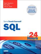
The following is an example using a phony table:
Watch Out!: Always Test Your WHERE Clauses
If you do not know how your particular implementation’s SQL optimizer works, the DBA does not know, or you do not have sufficient documentation, you can execute a large query that takes a while to run and then rearrange conditions in the WHERE clause. Be sure to record the time it takes the query to complete each time you make changes. You should only have to run a couple of tests to figure out whether the optimizer reads the WHERE clause from the top to bottom or bottom to top. Turn off database caching during the testing for more accurate results.
The following is the first query:
SELECT COUNT(*)
FROM TEST
WHERE LAST_NAME = 'SMITH'
AND CITY = 'INDIANAPOLIS';
COUNT(*)
----------
1,024
The following is the second query:
SELECT COUNT(*)
FROM TEST
WHERE CITY = 'INDIANAPOLIS'
AND LAST_NAME = 'SMITH';
COUNT(*)
----------
1,024
Suppose that the first query completed in 20 seconds, whereas the second query completed in 10 seconds. Because the second query returned faster results and the most restrictive condition was listed last in the WHERE clause, it is safe to assume that the optimizer reads the WHERE clause from the bottom up.
By the Way: Try to Use Indexed Columns
It is a good practice to use an indexed column as the most restrictive condition in a query. Indexes generally improve a query’s performance.
Full Table Scans
A full table scan occurs when an index is not used by the query engine or there is no index on the table(s) being used. Full table scans usually return data much slower than when an index is used. The larger the table, the slower that data is returned when a full table scan is performed. The query optimizer decides whether to use an index when executing the SQL statement. The index is used—if it exists—in most cases.
Some implementations have sophisticated query optimizers that can decide whether to use an index. Decisions such as this are based on statistics that are gathered on database objects, such as the size of an object and the estimated number of rows that are returned by a condition with an indexed column. Refer to your implementation documentation for specifics on the decision-making capabilities of your relational database’s optimizer.
You should avoid full table scans when reading large tables. For example, a full table scan is performed when a table that does not have an index is read, which usually takes a considerably longer time to return the data. An index should be considered for the majority of larger tables. On small tables, as previously mentioned, the optimizer might choose the full table scan over using the index, if the table is indexed. In the case of a small table with an index, you should consider dropping the index and reserving the space that was used for the index for other needy objects in the database.
Did You Know?: There Are Simple Ways to Avoid Table Scans
The easiest and most obvious way to avoid a full table scan—outside of ensuring that indexes exist on the table—is to use conditions in a query’s WHERE clause to filter data to be returned.
The following is a reminder of data that should be indexed:
• Columns used as primary keys
• Columns used as foreign keys
• Columns frequently used to join tables
• Columns frequently used as conditions in a query
• Columns that have a high percentage of unique values
Did You Know?: Table Scans Are Not Always Bad
Sometimes full table scans are good. You should perform them on queries against small tables or queries whose conditions return a high percentage of rows. The easiest way to force a full table scan is to avoid creating an index on the table.
Other Performance Considerations
There are other performance considerations that you should note when tuning SQL statements. The following concepts are discussed in the next sections:
• Using the LIKE operator and wildcards
• Avoiding the OR operator
• Avoiding the HAVING clause
• Avoiding large sort operations
• Using stored procedures
• Disabling indexes during batch loads
Using the LIKE Operator and Wildcards
The LIKE operator is a useful tool that places conditions on a query in a flexible manner. Using wildcards in a query can eliminate many possibilities of data that should be retrieved. Wildcards are flexible for queries that search for similar data (data that is not equivalent to an exact value specified).
Suppose you want to write a query using EMPLOYEE_TBL selecting the EMP_ID, LAST_NAME, FIRST_NAME, and STATE columns. You need to know the employee identification, name, and state for all the employees with the last name Stevens. Three SQL statement examples with different wildcard placements serve as examples.
The following is Query 1:
SELECT EMP_ID, LAST_NAME, FIRST_NAME, STATE
FROM EMPLOYEE_TBL
WHERE LAST_NAME LIKE 'STEVENS';
SELECT EMP_ID, LAST_NAME, FIRST_NAME, STATE
FROM EMPLOYEE_TBL
WHERE LAST_NAME LIKE '%EVENS%';
Here is the last query, Query 3:
SELECT EMP_ID, LAST_NAME, FIRST_NAME, STATE
FROM EMPLOYEE_TBL
WHERE LAST_NAME LIKE 'ST%';
The SQL statements do not necessarily return the same results. More than likely, Query 1 will return fewer rows than the other two queries and will take advantage of indexing. Query 2 and Query 3 are less specific as to the desired returned data, thus making them slower than Query 1. Additionally, Query 3 is probably faster than Query 2 because the first letters of the string for which you are searching are specified (and the column LAST_NAME is likely to be indexed). So Query 3 could potentially take advantage of an index.
By the Way: Try to Account for Differences in the Data
With Query 1, you might retrieve all individuals with the last name Stevens; but can’t Stevens be spelled different ways? Query 2 picks up all individuals with the last name Stevens and its various spellings. Query 3 also picks up any last name starting with ST; this is the only way to ensure that you receive all the Stevens (or Stephens).
Avoiding the OR Operator
Rewriting the SQL statement using the IN predicate instead of the OR operator consistently and substantially improves data retrieval speed. Your implementation tells you about tools you can use to time or check the performance between the OR operator and the IN predicate. An example of how to rewrite an SQL statement by taking the OR operator out and replacing the OR operator with the IN predicate follows.
By the Way: How to Use OR and IN
Refer to Hour 8, “Using Operators to Categorize Data,” for the use of the OR operator and the IN predicate.
The following is a query using the OR operator:
SELECT EMP_ID, LAST_NAME, FIRST_NAME
FROM EMPLOYEE_TBL
WHERE CITY = 'INDIANAPOLIS'
OR CITY = 'BROWNSBURG'
OR CITY = 'GREENFIELD';
The following is the same query using the IN operator:
SELECT EMP_ID, LAST_NAME, FIRST_NAME
FROM EMPLOYEE_TBL
WHERE CITY IN ('INDIANAPOLIS', 'BROWNSBURG',
'GREENFIELD'),
The SQL statements retrieve the same data; however, through testing and experience, you find that the data retrieval is measurably faster by replacing OR conditions with the IN predicate, as in the second query.
Avoiding the HAVING Clause
The HAVING clause is a useful clause for paring down the result of a GROUP BY clause; however, you can’t use it without cost. Using the HAVING clause gives the SQL optimizer extra work, which results in extra time. Not only will the query be concerned with grouping result sets, it also will be concerned with parsing those result sets down via the restrictions of the HAVING clause. For example, observe the following statement:
SELECT C.CUST_ID, C.CUST_NAME, P.PROD_DESC,
SUM(O.QTY) AS QTY, SUM(P.COST) AS COST,
SUM(O.QTY * P.COST) AS TOTAL
FROM CUSTOMER_TBL AS C
INNER JOIN ORDERS_TBL AS O ON C.CUST_ID = O.CUST_ID
INNER JOIN PRODUCTS_TBL AS P ON O.PROD_ID = P.PROD_ID
WHERE PROD_DESC LIKE ('P%')
GROUP BY C.CUST_ID, C.CUST_NAME, P.PROD_DESC
HAVING SUM(O.QTY * P.COST)>25.00
Here we are trying to determine which customers have sales of specific products over the total of $25.00. Although this query is fairly simple and our sample database is small, the addition of the HAVING clause introduces some overhead, especially when the HAVING clause has more complex logic and a higher number of groupings to be applied. If possible, you should write SQL statements without using the HAVING clause or design the HAVING clause restrictions so they are as simple as possible.
Avoiding Large Sort Operations
Large sort operations mean using the ORDER BY, GROUP BY, and HAVING clauses. Subsets of data must be stored in memory or to disk (if there is not enough space in allotted memory) whenever sort operations are performed. You must sort data often. The main point is that these sort operations affect an SQL statement’s response time. Because you cannot always avoid large sort operations, it is best to schedule queries with large sorts as periodic batch processes during off-peak database usage so that the performance of most user processes is not affected.
Using Stored Procedures
You should create stored procedures for SQL statements executed on a regular basis—particularly large transactions or queries. Stored procedures are simply SQL statements that are compiled and permanently stored in the database in an executable format.
Normally, when an SQL statement is issued in the database, the database must check the syntax and convert the statement into an executable format within the database (called parsing). The statement, after it is parsed, is stored in memory; however, it is not permanent. This means that when other operations need memory, the statement might be ejected from memory. In the case of stored procedures, the SQL statement is always available in an executable format and remains in the database until it is dropped like any other database object. Stored procedures are discussed in more detail in Hour 22, “Advanced SQL Topics.”
Disabling Indexes During Batch Loads
When a user submits a transaction to the database (INSERT, UPDATE, or DELETE), an entry is made to both the database table and any indexes associated with the table being modified. This means that if there is an index on the EMPLOYEE table, and a user updates the EMPLOYEE table, an update also occurs to the index associated with the EMPLOYEE table. In a transactional environment, having a write to an index occur every time a write to the table occurs is usually not an issue.
During batch loads, however, an index can actually cause serious performance degradation. A batch load might consist of hundreds, thousands, or millions of manipulation statements or transactions. Because of their volume, batch loads take a long time to complete and are normally scheduled during off-peak hours—usually during weekends or evenings. To optimize performance during a batch load—which might equate to decreasing the time it takes the batch load to complete from 12 hours to 6 hours—it is recommended that the indexes associated with the table affected during the load are dropped. When you drop the indexes, changes are written to the tables much faster, so the job completes faster. When the batch load is complete, you should rebuild the indexes. During the rebuild, the indexes are populated with all the appropriate data from the tables. Although it might take a while for an index to be created on a large table, the overall time expended if you drop the index and rebuild it is less.
Another advantage to rebuilding an index after a batch load completes is the reduction of fragmentation that is found in the index. When a database grows, records are added, removed, and updated, and fragmentation can occur. For any database that experiences a lot of growth, it is a good idea to periodically drop and rebuild large indexes. When you rebuild an index, the number of physical extents that comprise the index is decreased, there is less disk I/O involved to read the index, the user gets results more quickly, and everyone is happy.
Cost-Based Optimization
Often you inherit a database that is in need of SQL statement tuning attention. These existing systems might have thousands of SQL statements executing at any given time. To optimize the amount of time spent on performance tuning, you need a way to determine what queries are most beneficial to concentrate on. This is where cost-based optimization comes into play. Cost-based optimization attempts to determine which queries are most costly in relation to the overall system resources spent. For instance, say we measure cost by execution duration and we have the following two queries with their corresponding run times:
SELECT * FROM CUSTOMER_TBL
WHERE CUST_NAME LIKE '%LE%' 2 sec
SELECT * FROM EMPLOYEE_TBL
WHERE LAST_NAME LIKE 'G%'; 1 sec
At first, it might appear that the first statement is the one you need to concentrate your efforts on. However, what if the second statement is executed 1,000 times an hour but the first is performed only 10 times in the same hour? Doesn’t this make a huge difference in how you allocate your time?
Cost-based optimization ranks SQL statements in order of total computational cost. Computational cost is easily determined based on some measure of query execution (duration, number of reads, and so on) multiplied by the number of executions over a given period:
Total Computational Cost = Execution Measure * (number of executions)
This is important because you get the most overall benefit from tuning the queries with the most total computational cost first. Looking at the previous example, if we are able to cut each statement execution time in half, you can easily figure out the total computational savings:
Statement #1: 1 sec * 10 executions = 10 sec of computational savings
Statement #2: .5 sec * 1000 executions = 500 sec of computational savings
Now it is much easier to understand why your valuable time should be spent on the second statement instead of the first. Not only have you worked to optimize your database, but you’ve optimized your time as well.
Performance Tools
Many relational databases have built-in tools that assist in SQL statement database performance tuning. For example, Oracle has a tool called EXPLAIN PLAN that shows the user the execution plan of an SQL statement. Another tool in Oracle that measures the actual elapsed time of an SQL statement is TKPROF. In SQL Server, the Query Analyzer has several options to provide you with an estimated execution plan or statistics from the executed query. Check with your DBA and implementation documentation for more information on tools that might be available to you.
Summary
You have learned the meaning of tuning SQL statements in a relational database. You have learned that there are two basic types of tuning: database tuning and SQL statement tuning—both of which are vital to the efficient operation of the database and SQL statements within it. Each is equally important and cannot be optimally tuned without the other.
You have read about methods for tuning an SQL statement, starting with a statement’s actual readability, which does not directly improve performance but aids the programmer in the development and management of statements. One of the main issues in SQL statement performance is the use of indexes. There are times to use indexes and times to avoid using them. For all measures taken to improve SQL statement performance, you need to understand the data itself, the database design and relationships, and the users’ needs as far as accessing the database.
Q&A
Q. By following what I have learned about performance, what realistic performance gains, as far as data retrieval time, can I really expect to see?
A. Realistically, you could see performance gains from fractions of a second to minutes, hours, or even days.
Q. How can I test my SQL statements for performance?
A. Each implementation should have a tool or system to check performance. Oracle7 was used to test the SQL statements in this book. Oracle has several tools for checking performance. Some of these tools include the EXPLAIN PLAN, TKPROF, and SET commands. Check your particular implementation for tools that are similar to Oracle’s.
Workshop
The following workshop is composed of a series of quiz questions and practical exercises. The quiz questions are designed to test your overall understanding of the current material. The practical exercises are intended to afford you the opportunity to apply the concepts discussed during the current hour, as well as build upon the knowledge acquired in previous hours of study. Please take time to complete the quiz questions and exercises before continuing. Refer to Appendix C, “Answers to Quizzes and Exercises,” for answers.
Quiz
1. Would the use of a unique index on a small table be of any benefit?
2. What happens when the optimizer chooses not to use an index on a table when a query has been executed?
3. Should the most restrictive clause(s) be placed before the join condition(s) or after the join conditions in the WHERE clause?
Exercises
1. Rewrite the following SQL statements to improve their performance. Use EMPLOYEE_TBL and EMPLOYEE_PAY_TBL as described here:
EMPLOYEE_TBL
EMP_ID VARCHAR(9) NOT NULL Primary key,
LAST_NAME VARCHAR(15) NOT NULL,
FIRST_NAME VARCHAR(15) NOT NULL,
MIDDLE_NAME VARCHAR(15),
ADDRESS VARCHAR(30) NOT NULL,
CITY VARCHAR(15) NOT NULL,
STATE VARCHAR(2) NOT NULL,
ZIP INTEGER(5) NOT NULL,
PHONE VARCHAR(10),
PAGER VARCHAR(10),
CONSTRAINT EMP_PK PRIMARY KEY (EMP_ID)
EMPLOYEE_PAY_TBL
EMP_ID VARCHAR(9) NOT NULL primary key,
POSITION VARCHAR(15) NOT NULL,
DATE_HIRE DATETIME,
PAY_RATE DECIMAL(4,2) NOT NULL,
DATE_LAST_RAISE DATETIME,
SALARY DECIMAL(8,2),
BONUS DECIMAL(8,2),
CONSTRAINT EMP_FK FOREIGN KEY (EMP_ID)
REFERENCES EMPLOYEE_TBL (EMP_ID)
a. SELECT EMP_ID, LAST_NAME, FIRST_NAME,
PHONE
FROM EMPLOYEE_TBL
WHERE SUBSTRING(PHONE, 1, 3) = '317' OR
SUBSTRING(PHONE, 1, 3) = '812' OR
SUBSTRING(PHONE, 1, 3) = '765';
b. SELECT LAST_NAME, FIRST_NAME
FROM EMPLOYEE_TBL
WHERE LAST_NAME LIKE '%ALL%;
c. SELECT E.EMP_ID, E.LAST_NAME, E.FIRST_NAME,
EP.SALARY
FROM EMPLOYEE_TBL E,
EMPLOYEE_PAY_TBL EP
WHERE LAST_NAME LIKE 'S%'
AND E.EMP_ID = EP.EMP_ID;
2. Add another table called EMPLOYEE_PAYHIST_TBL that contains a large amount of pay history data. Use the table that follows to write the series of SQL statements to address the following problems:
EMPLOYEE_PAYHIST_TBL
PAYHIST_ID VARCHAR(9) NOT NULL primary key,
EMP_ID VARCHAR(9) NOT NULL,
START_DATE DATETIME NOT NULL,
END_DATE DATETIME,
PAY_RATE DECIMAL(4,2) NOT NULL,
SALARY DECIMAL(8,2) NOT NULL,
BONUS DECIMAL(8,2) NOT NULL,
CONSTRAINT EMP_FK FOREIGN KEY (EMP_ID)
REFERENCES EMPLOYEE_TBL (EMP_ID)
What steps did you take to ensure that the queries you wrote perform well?
a. Find the SUM of the salaried versus nonsalaried employees by the year in which their pay started.
b. Find the difference in the yearly pay of salaried employees versus nonsalaried employees by the year in which their pay started. Consider the nonsalaried employees to be working full time during the year (PAY_RATE * 52 * 40).
c. Find the difference in what employees make now versus what they made when they started with the company. Again, consider the nonsalaried employees to be full-time. Also consider that the employees’ current pay is reflected in the EMPLOYEE_PAY_TBL as well as the EMPLOYEE_PAYHIST_TBL. In the pay history table, the current pay is reflected as a row with the END_DATE for pay equal to NULL.