

Figure 9.1Pentagon of Power
The past couple of chapters explored controls that used limit switches for position feedback and manual adjustment of speed. There is a limit (pun intended) to the usefulness of such systems. Once you need more than a handful positions, easily adjustable positions, precise timing, or precise speed, your needs have outgrown simple controls. As we contemplate the Control point of the Pentagon of Power, the next step forward is a system that can take cue information and execute the cue automatically. A system that thinks in speed, acceleration, and distance. A system that automatically adjusts power to keep a constant speed. A system that knows when to start deceleration to land perfectly on spike. Sounds great. Where do we start? Where all good things start: better hardware and Calculus.
Way back in Chapter 6, we discussed encoders and explored the plethora of options in those sensors. To implement a more sophisticated control output, we need a more sophisticated feedback sensor than the limit switches we’ve been using in the past couple of chapters. Encoders are the answer. Rather than just sensing when the machine arrives at a discrete location, encoders sense the movement of the machine constantly. This feedback signal will be used not only for positioning, but also to sense the speed and direction of a machine.
To have an accurate picture of how the control’s command signal is affecting the machine, the encoder must be physically connected to either the machine or the scenery that the machine is moving. As we’ll see, the control can only operate effectively when the coupling between input command and output reaction is tight. Any sloppiness in that connection will create an unstable control loop and make accurate, smooth movement difficult or impossible. When troubleshooting a system that is running erratically, the first spot for potential issue is the mechanical link between the machine and the encoder. In programming, there is a term used to describe the effectiveness of data and processing algorithms: GIGO, which means Garbage In, Garbage Out. It applies equally to motion control. If the encoder feedback into the control is not accurate, there is no way to produce an accurate output command signal.

Figure 9.2Encoder attached to machine

Figure 9.3Encoder attached to scenery
As previously mentioned, there are two major families of encoders: absolute and incremental. There are advantages to both, but for the sake of our discussion on control loops, it doesn’t matter. What matters is that the encoder produces data in a format that can be deciphered by the controller. If the controller only accepts incremental encoders, that’s what is needed, and vice versa. The point of an encoder is to represent motion as an electrical signal and that signal must be compatible with the controller you select.
The encoder closes the loop between the controller and machine: the output from the control produces movement, and that movement is observed by the control. When you hear the term “closed-loop system,” you can be assured that an encoder is installed. By contrast, an “open-loop system” does not use an encoder and the control is not able to observe the motion of the machine. We are only concerned with closed-loop systems here.

Figure 9.4Closed-loop control

Figure 9.5Open-loop control
Chances are you’ve heard the term “PID loop” (pronounced P-I-D) bandied about. PID stands for Proportional, Integral, and Derivative, which may, if you’re like me, vaguely remind you of a distant Calculus class. If you are math-averse, the good news is that you don’t need to solve any equations to understand the concepts in PID control. If you are mathyTM by nature, then rejoice in the practical application of some very cool math. But before we get into the specifics of how this stuff works, we need to define the problem we want to solve and get a little vocabulary under our collective belts.
The control system has a goal. In our case, move a motor from here to there. With that goal, the control generates a plan of how to get from here to there. Using this idyllic plan, the control sends an output to the amplifier and then watches the signal from the feedback device to sense how the system is responding. The control output signal is known as the command. Since the world is an imperfect place, the reaction of the system is seldom perfect. The control compares actual system response to its calculated ideal state. The difference in desired and actual state is known as the error. The control then applies a correction to reduce the error, and the whole thing starts again.

Figure 9.6PID loop
The cycle of command, calculate error, and apply correction is the “loop” in PID loop. It is an algorithm for a self-correcting control system. Automation systems employ this algorithm to create accurate movements, but it is widely used in other industrial processes that need to self-correct for any error. Chemical processes use it to maintain proper pH levels and heating systems use it to maintain temperature. To grasp the sophistication of the algorithm, we should study the concept from the most fundamental and build on the idea until we understand how each term functions and enhances the control loop.
Mapping Motion
A control loop used to move a machine from here to there needs to create a map of the movement based on the starting position, ending position, desired speed (velocity), acceleration, and deceleration. The loop cycles rapidly at a fixed timing interval, and the map is used to check the desired position of the machine during any cycle. Assuming a constant acceleration, Newtonian physics equations can be used to determine the relationship between time, position, acceleration, and speed. Here’s a list of the pertinent equations:
| Equation | Calculate | Known | ||
| v = vo + at | velocity | acceleration, time | ||
| x = ½(v + vo)t | position change | velocity, time | ||
| t = x / v | time | velocity, position change, zero acceleration | ||
| x = vot + ½at2 | position change | acceleration, time | ||
| v2 = vo2 + 2ax | velocity | acceleration, position change | ||
| a = (v – vo)/t | acceleration | speed, time | ||
| t = (v-vo)/a | time | speed, non-zero acceleration |
where:
| Symbol | Meaning |
| v | final velocity |
| vo | initial velocity |
| x | position change |
| a | acceleration |
| t | time in seconds |
To understand how the control loop does its magic, we will manually walk through the calculations. You wouldn’t need to perform these calculations to operate an automation system, but you may need to understand the math if you want to build your own sophisticated control.
A basic cue starts at known position with zero velocity, accelerates to the programmed speed, travels a bit, and then decelerates, back down to zero speed, landing at the programmed position. A graphical representation of that sentence sheds some light on how to approach this problem.

Figure 9.7Motion graph of speed over time
We have three distinct movements, or trajectories, to solve for: acceleration ramp (positive acceleration), constant speed (zero acceleration), and deceleration ramp (negative acceleration). In order to find the desired position at any point in time, we must first determine the boundaries of each movement so we have the correct parameters to plug into the motion equations. To find the boundaries, we will calculate the length of each movement to determine the starting and ending time. We will also calculate the starting and ending position of each movement. Combining those calculated values with the given values of the cue, we can then derive the desired position at any point in time. Let’s work through an example.
Consider a cue that starts a wagon offstage at position 0, and moves 200 in onstage at a speed of 20 in/sec. We would like a 2-second ramp up to get moving quickly out of the wings, but a more graceful 4-second ramp down once the wagon is in sightlines. Charts of what we know and what we need to calculate look like this:
| Symbol | Value | Meaning | ||
| v1o | 0 in/sec | initial velocity | ||
| v1 | 20 in/sec | final velocity | ||
| t1 | 2 sec | duration | ||
| t1start | 0 sec | starting time | ||
| a1 | ? in/sec/sec (or? in/sec2) | acceleration | ||
| x1 | ? in | change in position |
| Symbol | Value | Meaning | ||
| v2o | 20 in/sec | initial velocity | ||
| v2 | 20 in/sec | final velocity | ||
| t2 | ? sec | duration | ||
| t2start | t1 | starting time | ||
| a2 | 0 in/sec/sec (or? in/sec2) | acceleration | ||
| x2 | ? in | change in position |
| Symbol | Value | Meaning | ||
| v3o | 20 in/sec | initial velocity | ||
| v3 | 0 in/sec | final velocity | ||
| t3 | 4 sec | duration | ||
| t3start | t1 + t2 | starting time | ||
| a3 | ? in/sec/sec (or? in/sec2) | acceleration | ||
| x3 | ? in | change in position |
To find a1:
To find a3:
To find x1:
To find x3:
To find x2, recall that the cue moves a total of 200 in:
With x2 known, we can now calculate the duration of the constant speed movement:
We can now fill in our initial chart of values completely:
| Symbol | Value | Meaning | ||
| v1o | 0 in/sec | initial velocity | ||
| v1 | 20 in/sec | final velocity | ||
| t1 | 2 sec | duration | ||
| t1start | 0 sec | starting time | ||
| a1 | 10 in/sec/sec | acceleration | ||
| x1 | 20 in | change in position |
| Symbol | Value | Meaning | ||
| v2o | 20 in/sec | initial velocity | ||
| v2 | 20 in/sec | final velocity | ||
| t2 | 7 sec | duration | ||
| t2start | 2 sec | starting time | ||
| a2 | 0 in/sec2 | acceleration | ||
| x2 | 140 in | change in position |
| Symbol | Value | Meaning | ||
| v3o | 20 in/sec | initial velocity | ||
| v3 | 0 in/sec | final velocity | ||
| t3 | 4 sec | duration | ||
| t3start | 9 sec | starting time | ||
| a3 | -5 in/sec2 | acceleration | ||
| x3 | 40 in | change in position |

Figure 9.8Velocity over time
With the boundaries established for each movement in the cue, we can tackle the deceptively simple question of the motor’s position at any given time. Let’s walk through the process to find the motor position 10.5 seconds after the start of the cue. First, we must determine which movement we are dealing with for the desired time. A quick scan of our charts shows that at 10.5 seconds, cue is in the Deceleration Ramp. That movement has a non-zero acceleration, so we solve for position change using an equation that involves acceleration and time:
t in this equation is relative to the start time of the movement:

Figure 9.9Deceleration ramp profile
The position change is relative to the start position of the movement. To determine the absolute position of the motor at 10.5 seconds, we sum all the position changes with the starting position:
The motion control loop will run that calculation thousands or millions of times per second, depending on the specific controller, to figure out where the machinery should be and calculate the difference between the actual position the feedback sensor is reporting to determine the position error. Though a bit tedious, the math isn’t complex, and computers are really good at doing tedious math quickly.
Now that we know how to compute the position error at any point in time, we must devise a strategy to reduce, or, hopefully, eliminate, the position error. Let’s take a look at a few different strategies for eliminating position error.
On–Off Control
A basic thermostat operates by On–Off control. When the temperature falls below the set threshold, the thermostat turns on to fire the furnace. As the temperature in the room rises and passes the setpoint, the furnace is turned off. In temperature control, error is the difference between the desired temperature you set on the thermostat and the actual temperature read by the thermometer. Turning on/off the furnace at full capacity yields acceptable performance for a furnace in a small building, but it is too primitive for motion control.
Imagine a motion controller that just turned a winch on and off at full speed to eliminate position error. Its attempt at an acceleration ramp would pulse the scenery across the stage alternatively running at full-speed and slamming on the brakes. Clearly On–Off control is not sufficient. The calculations to map the movement give plenty of input information to the control loop to determine the position error, but if the only output the loop can generate is a binary on/off, the control algorithm is lacking the tools it needs to make smooth corrections to the motion.
Proportional Control
The amplifiers we use in automation are fully capable of variable speed. When commanded to run at 50%, they do so. Dial the speed down to 5%, and they obey, dutifully slowing down the motor to a crawl. Our control algorithm should take advantage of this by producing a varying signal to command the motor to catch up or slow down at the appropriate times. A proportional control algorithm produces an output signal that is proportional to the position error input captured by the encoder. As the loop dutifully calculates the position error, it generates a corrective action based on the magnitude of that error. A large error generates a large correction. If a machine is falling behind the desired position, the proportional control will produce a large command signal to reduce the error. As the machine catches up to the desired position, the command signal is reduced proportionally to lessen the energy provided to the machine. A small error results in a proportionally small corrective action. This is an intuitive solution: big error = big correction, small error = small correction.

Figure 9.10Position error
To govern the magnitude of “big” and “small” corrections, a coefficient is introduced to the algorithm. Proportional Gain is a constant that is multiplied by the current position error to affect the output signal of the control loop. A gain of 0 would produce no output signal regardless of the position error. A gain of 1 produces a straight 1:1 ratio of input error to output signal.1 A gain greater than 1 amplifies the output correction. Mathematically:
The output at any instantaneous time (t) equals the product of Proportional Gain (Kp) and the position error at time (t). As you can see from this formula, Proportional Gain only acts on the current position error as calculated during a single cycle of the control loop. On the next iteration of the control loop, a new Position Error will be calculated and any previous correction is lost in the mists of time. Proportional Gain lives in the now; the past is best forgotten.
You may be nodding along at this point wondering, Where does Kp come from? What is that value? Good question. The Proportional Gain is a constant that you determine and provide to the control loop. Setting this gain, and others, is known as “tuning” the control loop. In my years of both producing automation systems, and providing technical support for others embroiled in automation woes, I’ll put a stake in the ground and state that “tuning” is initially one of the hardest and weirdest aspects of getting a motion control system working up to expectations.
Proportional Gain is dependent on the system response, as are the other gains yet to come. The command signal produced by the control loop is sent out to the amplifier, the amplifier spins the machine, which in turn spins the encoder. The motion of the encoder generates an electrical signal that describes the actual movement of the machine and that signal is feed back into the control loop.

Figure 9.11Control loop
The amount of gain required is related to the amount of energy that must be expended to move the encoder. That quantity of energy is largely governed by two characteristics of the mechanical system: the resolution of the encoder and the force required to move. Of these two factors, in my experience, the resolution of the encoder plays a bigger role because the amplifier is pretty good at matching its output power to the command signal of the control. Consider the following two wildly different encoder disks fastened to the machine. The first has 4 counts per revolution, the second has 10,000. If the control system has to correct for a position error of 1 count, in the first example it must generate a command signal that prods the amplifier to spin the motor a quarter of a rotation, or 90 degrees. The second system, with a much finer resolution, merely has to generate a command signal that produces 0.036 degrees of rotation. Clearly the second system requires much less energy to correct for the position error. Since the magnitude of the correction is governed by the Proportional Gain, the second system, with the fine resolution encoder, will have a much smaller gain than the first, coarse resolution system.

Figure 9.12High-resolution vs. low-resolution encoders
A sneakier problem surrounds coarse resolution encoders and the control loop. The control loop executes very quickly, sampling the encoder for position changes every iteration and calculating the error. If the encoder resolution is so coarse that it doesn’t advance in between control loop cycles, the control loop interprets the dearth of encoder counts to mean that the machinery isn’t moving. In fact, the machine is moving, it just hasn’t moved enough to trigger an encoder signal because the encoder is in between positions. The control loop will aggressively attempt to advance the machine to catch up, which can cause erratic motion. Any disconnect between the output of the control loop and the feedback signal creates a system that is difficult to tune because the mathematical model is being hamstrung by poor component response. A higher resolution encoder makes tuning easier.
Why not just set the Gain to the max value? More power is always better, amiright? No, gain settings are much closer to Goldilocks and the Three Gains: they must be “just right.” Consider an excessively high Proportional Gain. When the Position Error is calculated, an error of -1 is detected, but because the Proportional Gain is high, a correction of +10 is produced. That output is sent to the amplifier and the motor lunges forward. On the next iteration of the control loop, the Position Error is now +9 and so an equally large reverse correction is applied. The motor is now oscillating back and forth, consistently overshooting the desired position in both directions. This action may start as the sound of a slight grumble in a winch or turntable, but if the telltale signs are ignored, and you continue to increase Proportional Gain, the machine will quickly begin wrenching the scenery back and forth in a frightening manner. At this level, we have effectively created an ON/OFF control loop because the gain is so high. The correct gain setting should be low enough to prevent violent oscillation.

Figure 9.13Command signal oscillation
Ok, how about we just set the Proportional Gain to a minimal value to avoid the pitfalls of too high a gain? Nope, that doesn’t work either. If the gain is too low, the machinery will always be starved of the power it needs to effectively execute the cue. The corrective actions will be too small and the scenery will forever be falling behind the desired position on each iteration of the control loop. This sloppy behavior makes the timing of cues completely inaccurate. To accurately predict the time a cue will take to complete, the machinery has to perform near to the theoretical ideal that is used to calculate the desired position. If the performance of a poorly tuned machine is critically inaccurate, any tightly timed sequences on stage will be, at best, displeasing but at worst can lead to collisions.

Figure 9.14Sluggish command signal
Proportional Gain needs to be set just below the level that would create oscillation. You find that level by iteratively running a machine back and forth and increasing Proportional Gain until you find a value that produces crisp, accurate movement without oscillation. Or, you press a little too far, find the point that the machine becomes unstable and back down a touch. In most vanilla-flavored automation rigs, this process should not take more than 15 minutes once you get the hang of it.
Before we move on to the next, more complex terms of PID control, I’d like to point out that much of the time a Proportional Control loop is all that is required. Many of the mechanical systems that we use on stage aren’t so fussy as to need the other terms: Integral and Derivative. Even if you do find that you can’t achieve smooth, accurate motion with just Proportional Gain, it is where you should always start. The Proportional term of a PID control loop is the easiest to understand and has the most predictable impact. As you tune a PID system, one term should be adjusted at a time. Making changes to all three terms at once and determining which term is affecting the performance of the machinery is an exercise in frustration. Start simple and methodically add layers to the control loop as needed. Once your requirements are met, stop tuning.
Integral Term in PID
The Proportional term in a PID control loop acts only in the instant of the current iteration of the control loop. Effective as it is, there is a significant limitation in the Proportional term since it can’t see a historical error in the command output. For the Proportional term to add any corrective action, and thereby create a non-zero command signal, some amount of position error must exist. If the position error drops to zero, so does the command signal. As a result, there is always some amount of position error to keep the system operating. In a well-tuned Proportional system, this results in a constant, steady position error. This steady-state error can be eliminated by adding a historical perspective to the control loop.

Figure 9.15Long-running steady state error
The integral term sums the position error over the length of the movement and uses that data to provide a correction. If you remember from Calculus, integral computes the area beneath a curve. A graph of position error over the course of a cue shows an area beneath it that represents the history of position error. The integral term uses that area of position error and multiplies it by Integral Gain to create a correction to the command signal that is combined with the Proportional term. The discrete time equation describes the Integral term used in the LM628 motion processor (one of many motion processors commercially available):

The significant concept of the Integral term is that its contribution to the command signal will grow as more time passes with an existing position error. In practice, this has the very useful property of correcting the position of a machine that is unable to get onto the programmed spike. With every passing cycle of the control loop, the command signal will grow and eventually enough energy will exist to push the scenery to the expected position. In a machine that can’t tolerate a higher Proportional Gain to reach target position, the integral term, with an appropriate gain, can get the job done.

Figure 9.16Integral term growing over time
Because the Integral term is summing the position error over time, the magnitude of its correction can grow quite large especially when a rapid change in speed is desired. The resulting correction can cause an overshoot and trigger oscillation in the machinery. This is known as Integral Windup. Once the oscillation starts, the instability can increase unless another aspect of the control algorithm clamps down on the command signal. Many implementations of PID control will include an Integral Limit that places an upward boundary on the Integral term and avoids Integral Windup.
In practice, Integral Gain can be added to a system that is having trouble completing cues on target with just Proportional Gain. Since its strength grows as time goes, it will eventually produce the energy needed to reduce position error.
Derivative Term in PID
The final term in PID is Derivative. If Integral is considering at the area beneath the curve graphing position error over time, Derivative is acting on the slope of that curve at any instant.

Figure 9.17Derivative term, slope of position error
Like the Integral term, the Derivative term considers the historical performance of the machine during the cue and uses that information to generate its contribution to the command signal correction. Because it is considering the slope of the position error, it is anticipating the trend of position error. If position error is getting worse, then the Derivative term correction will increase in magnitude. Conversely, if position error is improving, its correction will decrease.
To put it another way, the Derivative term is effective when the rate of position error is changing. We see this come into play usually just when the load on a scenic piece changes during a cue. For instance, a turntable with large number of the cast stepping on and off during a cue. Since those instances are rare, in practice the Derivative term is seldom used and can be tricky to set without introducing unwanted oscillation.
PID Summary
PID control is an algorithmic, self-correcting system. While it can be used to control many processes, we use it for motion control to correct for position error. Amplifiers (VFDs and servo amplifiers) use a PID loop to correct for speed errors and thereby maintain the speed command from the controller. An impressive, if not instantly obvious, feature of PID control is that systems have no need to know the percentage of “full-speed” to execute accurate motion. It’s natural to think of automation systems measuring speeds like lighting consoles measure light intensity, but that’s a naïve view. Motion controllers instead command motors to go only faster or slower and automatically correct based on the machine’s response to those commands. Given the limitless mechanical configurations, this sophistication in control is a huge advantage of PID systems. You can command two radically different machines, with different mechanical speed reducers, and different encoder resolutions, to move in unison. A PID loop on each machine will dutifully drive each machine to match speeds, though one may be running at 10% capacity and the other 90% capacity. Calculus and better hardware: two great tastes that go great together.
PID control theory is so broadly applicable and widely used in motion control that a large number of options exist that can be purchased and installed on stage.
Stagehand Mini2TM

Figure 9.18Stagehand Mini2TM
Source: Courtesy of Creative Conners
The Stagehand Mini2TM is a controller developed at Creative Conners specifically for stage automation. It houses two Stagehand motion controllers in a rackmount package. The Stagehand Motion Controller is based around the venerable Texas Instruments LM628 or LM629, which are monolithic ASICs (application specific integrated circuits) designed for motion control. Each channel on the Mini2 accepts incremental encoder input and outputs either +/-10 VDC or 0–5 VDC to command the speed and direction of an amplifier. Unlike the other Stagehand devices from Creative Conners, the Mini2 does not include a motor amplifier, which makes it interesting here since it is purely a control device. As with all Stagehand control devices, the Mini2 can be easily programmed to run cues through the SpikemarkTM cueing software.
Beckhoff PC

Figure 9.19Beckhoff embedded PC
Source: Courtesy of Beckhoff Automatiioon GmbH
Beckhoff has become a popular manufacturer of industrial PCs that combine the rich programming capability of PCs and the industrial, hardened I/O of PLCs. Combined with the Beckhoff TwinCAT programming interface and an impressively broad assortment of expansion modules, Beckhoff PCs can be configured to act as PID motion controllers with just about any interface for encoder feedback and speed signal output by adding on expansion slices and configuring the hardware through the Visual Studio programming software. There is no inherent way to write cues for the Beckhoff PC, but several commercial systems use Beckhoff components under the hood (Hudon Scenic Studio’s HMC and TAIT’s Navigator to name a couple), or you could develop your own.
PLCs

Figure 9.20Modicon PLC
PLCs have long included PID control loops as functions of higher-end models, but these days even many entry-level PLCs include the software features to run a PID control loop. Product lines like the Schneider Modicon have enough capability to function as a motion controller at relatively low cost. To accept encoder input, and generate command signal output, you can add on the appropriate modules to match your system needs. For instance, high-speed digital input modules can be used to capture incremental encoder pulses and analog output modules can be programmed to generate the command signal. Or, use digital inputs to capture an absolute encoder interface and a serial output to generate a digital speed command. The options are open, but require some additional effort to develop the code to tie the bits together.
VFD and Servo Amplifiers

Figure 9.21Mitsubishi A800
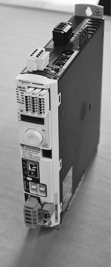
Figure 9.22Schneider Lexium 32C
At the higher end of VFDs, and mid- to high-end servo drives, the amplifiers contain enough control smarts to execute point-to-point positioning and include a PID control loop on-board. The advantage here is that the hardware already exists and doesn’t require additional purchase. The disadvantage is that all the software you will need to develop to make the drive execute cues will be forever tied into a single manufacturer’s amplifier. In some situations that compromise is reasonable, and in others it may be unacceptable since the lock-in to a particular manufacturer and type of prime mover can be awfully limiting. This lock-in is somewhat mitigated with the rise of the EtherCAT protocol developed as an open-standard by Beckhoff and implemented by many industrial equipment manufacturers.
Standalone Motion Controllers
There are a number of standalone motion control computers that are purpose-built for PID control. Galil Motion Control produces the DMC-XXX series of standalone motion controllers that can have trajectory information loaded over Ethernet or RS-232 and output analog command signal or step and direction. Parker-Compumotor produces the 6K motion controller that similarly can be programmed over Ethernet or RS-232 and outputs either analog command signal or step and direction. In years past, these types of products would have been a viable, or even preferred, component for developing an automation system. However, with the rise of EtherCAT master controllers from Beckhoff and other manufacturers, the advantage of these dedicated motion controllers is unclear. Perhaps there are still applications, but I think the burden is now to figure out the exceptional circumstances that require these devices. In fact, both Galil and Parker-Compumotor have EtherCAT master products that would seem to be a better choice for future development rather than their legacy products.
Detecting Encoder Failures and Obstructions
PID control loops are excellent at self-correcting for position error and they keep a machine on track as it moves across the stage. The simple loop of checking position, calculating the position error, and applying a correction makes no allowance for stopping the loop when something has gone wrong. As we’ve seen, the PID loop has one way to correct for a position error deficit – apply more power to the machine. That works very well if the source of the position error is a motor that isn’t being given enough power by the amplifier to keep moving, but it is disastrous if either the encoder has failed or the machine is stuck.
If the encoder stops sending output pulses, the position error will start growing rapidly. The machine is still moving, but the control loop can’t see the movement. The lack of encoder pulses could be caused by an encoder that has lost the magic smoke,2 a severed cable, loose solder joint, or set screw that has wiggled loose and released the physical connection between the machine and encoder shaft. The control loop does what it knows to do: send a higher command signal to reduce position error. In this case, the machine rapidly accelerates to full speed and keeps going until a limit switch is hit, or the scenery attached to the machine hits an immovable object. Not good.
Alternatively, the encoder may be functioning properly, but the machine can’t move because either the machinery or the scenery attached to it is physically jammed. In this situation, the control loop is dogged in its desire to reduce position error and will continue to pump out higher and higher command signal. Eventually, hopefully, a protective device will interrupt power to the circuit to prevent serious electrical damage, but considerable physical damage may already have been done.
In either situation, we need a mechanism to turn off the PID loop when the position error grows beyond reason. The control should implement an allowable position error threshold that, when exceeded, will cause the PID loop to be shut off, will stop the prime mover, and will alert the operator to the fault. In the Stagehand/SpikemarkTM system, we call this feature Abort on Position Error with a settable window for that position error. Other systems have different names, but all provide this same functionality, as should you if you create your own control.
There are other common occurrences that require the PID loop to be disabled. Striking a limit switch should kill the PID loop. Once a limit has been reached, clearly something has gone awry and not only should the machinery stop, but the PID loop should be stopped as well. Without explicitly stopping the PID loop, as soon as the limit is cleared, the control will attempt to get back on track with its last programmed directive, which will likely lead to it ramming full-speed into the same limit switch.
Manually jogging a motor is another occurrence in which the PID loop should be disabled. Otherwise, as soon as you flip the system back over to PID control, the motor will try to regain the last commanded position, in a hurry.
And finally, an Emergency Stop should remove power from the machine, but it also needs to disarm the PID loop. If the PID loop is not disabled, the position error will keep growing and growing while the Emergency Stop is engaged. As soon as the Emergency Stop is released, the machine will shoot off at full-speed, trying to catch up to where it was supposed to go in the previous cue. Early in my career, I worked for a large commercial scene shop and I started to design the second version of their automation control system. When I was testing their first implementation, I noted that their Emergency Stop was more of an “E-pause.” The big red button lifted power to the machines, but would not automatically disable the PID loop. If the operator forgot to manually shut off the control loop, releasing the E-stop caused everything to spin seemingly uncontrollably. The first time I experienced it, I was luckily in a warehouse by myself with some test equipment, but even in that controlled circumstance it scared the heck out of me. It’s alarming to see that much horsepower take off at full-speed. We fixed the system, but I point it out because it is possible to overlook and these considerations need to be made. A pre-packaged scenic automation system will have these important issues engineered properly, but if you are going to create a system, however small, you need to account for all of these scenarios.
The command signal output of the PID loop represents the desired speed of the machine and the direction of travel. The electrical shape that the signal takes varies by motion controller and should be matched to the command input expected by the amplifier. Most often this choice is dictated by some existing piece of hardware, or by the piece of hardware or software you are most passionate about using. For example, you may have an existing collection of VFDs that take 0–5 VDC speed with switch closures for forward and reverse. It would then make sense to select a motion controller that has a 0–5 VDC speed output. Or perhaps you want to use a specific piece of cueing software and the compatible motion controllers output +/-10 VDC speed and direction, so you search for amplifiers that will accept that speed signal as an input. Knowing the common language of the software, motion controller, and amplifier is critical since it is easy to end up with a pile of expensive components that don’t talk to each other.
Analog Signals
Analog signals have long been the lingua franca between control and amplifier. There is a marvelous simplicity in the analog format. The magnitude of either a low-voltage or low-current signal of a known range is used to describe the desired percentage of full speed that the amplifier should follow. The amplifier can be changed out at any time and the control need never be the wiser. A VFD, a servo amplifier, a DC regen drive, and a hydraulic proportional valve can all follow the same simple analog command. Just as the amplifier can be swapped out, so too can the control. Rather than a sophisticated PID controller, a simple power supply and pot can be used to generate the speed command, making it very easy to create a manual control interface that can be flipped into action when you need to override the cue control system. Many motion controllers provide an analog output signal and can therefore be exchanged without affecting the amplifier. This loose coupling exists in some digital interfaces as well, but not nearly so simply as in the analog counterparts.
The two biggest pitfalls of analog speed signals are noise corruption and transmission length. Analog signals are susceptible to interference from power sources that generate electrical noise, such as VFDs, servo drives, etc. This poses a bit of a problem if the signal used to control the amplifier is adversely affected by the operation of the amplifier. The longer the analog signal wires are, the more likely the signal is to be affected by interference or simply degrade because of the impedance of the conductors. In practice, this means that analog control wires need to be well shielded, kept as short as possible, and isolated from the power lines of amplifiers.
The bipolar 10 VDC speed signal is very common in both motion controllers and amplifiers. The voltage describes the speed and direction over just two wires. 0 VDC is a zero-speed command, -10 VDC is full-speed reverse, +10 VDC is full-speed forward, anything between is a percentage of full-speed. In addition to the speed command, a pair of wires is used to signal an ENABLE. The ENABLE signal is closed when the motion control wants the amplifier to pay attention to the speed signal. This additional step helps diminish the likelihood of unintended motion caused by interference on the speed command wires. If the amplifier were constantly listening to the speed command, then stray voltage introduced on the wires from a noisy power distro or wireless transmitter could initiate movement. If the ENABLE signal is open, any voltage on the speed command wires will be ignored.

Figure 9.23Bipolar control wiring example
Bipolar speed signal input is found in most servo amplifiers and proportional valve drives, but is often reserved for the more expensive VFDs and DC drives. In the mid-range and low-end VFDs, it is more common to find unipolar speed signal input with a separate set of digital signal inputs for direction. This command signal splits the speed magnitude into an analog voltage, either 0–10 VDC or 0–5 VDC, and the direction is selected by closing either a forward or reverse circuit. Some drives will use the direction selection as the ENABLE signal, or allow for a discrete ENABLE signal.

Figure 9.24Uni-polar control wiring example
While the previous two command signals use voltage to describe desired speed, current can also be used. The variable current format is more common in analog sensor feedback, but it is available on many VFDs and DC drives. Like the unipolar voltage variant, the current signal requires a separate digital signal to select direction. An interesting benefit of the 4–20 mA signal is that 0% speed is indicated by a 4 mA current. Because there is a constant, low-current signal when all wires are connected, signal loss can be determined if the current signal drops to 0 mA.

Figure 9.254–20 mA control wiring example
Digital Signals
The limitations of analog signals, transmission length, and interference, are mitigated by digital techniques. Additionally, many digital signals offer richer programming interfaces and additional data beyond simple magnitude and direction. With these advantages comes an increase in complexity, though as long as you select components that speak the same digital language, that complexity may be of little importance.
Originally developed for stepper drives (see Chapter 5), the Step and Direction digital format is used by other amplifiers and controllers. In this signal format, the position is described by a stream of digital pulses, each pulse indicating a fixed distance to travel. The speed of the pulse stream describes the speed of the movement. The direction of travel is indicated with a single, separate digital signal where high indicates a forward movement, and low indicates a reverse movement.

Figure 9.26Step and direction example
The CANopen protocol is much more than a speed command format. It is based on the CAN (Controller Area Network) physical layer and offers a high-level protocol to do lots of motion-related stuff. All that “stuff” is best left for discussion later in our Networks chapter (Chapter 12), but it’s worth mentioning here as a viable protocol for just sending speed commands. CANopen, like most digital signals these days, is transmitted serially, meaning that the bits are sent one after another on a signal wire rather than sending multiple bits simultaneously over many wires. You needn’t worry about how it works, the protocol takes care of insuring it does work; the key point is that many different pieces of information can be sent over just a few wires. The CANopen protocol defines a series of digital telegrams that can be sent from a master controller to as many as 127 slave devices. Depending on the defined role of the slave device, a series of PDO (Process Data Objects) are defined that can communicate the desire of the master to be executed by the slave. For example, a CANopen servo drive will respond to the PDO telegram for velocity setpoint. Provided you have two drives that both implement the CiA 402 (CAN in Automation) standard correctly, you can swap out amplifiers and the speed signal will be understood.

Figure 9.27CAN wiring example
Developed in 1979 by Modicon (now Schneider Electric) as a protocol for communication between their PLCs, Modbus is an open standard commonly used to connect industrial devices. A Modbus master can connect to as many as 245 slave devices. A Modbus network has a single master that makes requests for data from slave devices. Since it was originally developed for PLCs, the protocol specifies data as either coils or registers. There are four tables of data in a Modbus slave. A read-only and read/write table of coils 0–9999, and a read-only and read/write table of data registers 0–9999. An amplifier that implements Modbus will have a data register to hold the desired speed, another for acceleration time, and a coil to initiate motion in either the forward or reverse direction. By writing to the correct data registers and then setting the coil values you can control the speed and direction of the motor wired to the amplifier.
The protocol does not define a physical layer, only the application layer, so Modbus can be transmitted over various electrical networks. The most common transport layers for Modbus are RS-232 and RS-485. More recently, Modbus/TCP allows for Modbus communication over Ethernet networks. The master and slave device needs to support the same physical layer to wire up and communicate correctly.
A decade after Modbus, Profibus was introduced with ambitions to create a protocol capable of running all facets of an automated system and distinguishes families of devices through profile descriptions. Like the fieldbus protocols discussed above, an amplifier with a Profibus interface can have speed and direction commanded by a Profibus controller. Profibus is a very rich network protocol, and while capable of sending simple speed commands to an amplifier, more complex system information can also be trivially transmitted.
Beckhoff presented the EtherCAT protocol in 2003 as an Ethernet-based solution for automation communication with unmatched timing capability and large capacity for slave devices (65,536). EtherCAT is rapidly becoming a popular fieldbus for automated devices and is available either standard or as an add-on module in many amplifiers. If you are using an EtherCAT master computer, an EtherCAT slave can have its speed and direction set digitally over the protocol. As we’ll see in the Networks chapter (Chapter 12), EtherCAT can also describe synchronization between multiple motors and access sensor information from digital and analog devices as well as bridge to other network protocols; it’s very sophisticated.
Let’s continue our trend of assembling a representative system, now with a PID motion controller. As we build up in complexity, note that many of the components in the Pentagon of Power remain the same as simpler assemblies. Let’s work under the same premise as Chapter 7 and imagine that the machine is a traveler track winch with an AC induction motor.
Pentagon of Power Components

Figure 9.28Mitsubishi D700
The Mitsubishi D700 amplifier from Chapter 7 can continue to serve as our machine power source. Now is a good time to point out the communication options available on the D700 to set the desired speed from the motion controller. As you remember, we were previously commanding the speed with a simple knob, but now we need the motion controller to take over that responsibility. Clearly it requires one of the aforementioned command interfaces. This VFD will accept analog speed command, Modbus, or Mitsubishi’s proprietary CC-Link protocol. The controller needs to be matched with at least one of these protocols. Here, we’ll use the analog interface since it is both ubiquitous across many motion controllers and simple to implement.
The D700 only accepts a unipolar analog speed command, rather than the bipolar speed command found in higher-end models (such as the A800 from Mitsubishi). While not terribly critical for our performance, it is important to know these restrictions to insure compatibility between control and amplifier. What’s the difference? The unipolar signal can only express the magnitude of the required speed, not the direction. Whereas the bipolar signal uses the voltage polarity significantly (positive is forward and negative is reverse), the unipolar signal requires additional digital signals for direction. This format is sometimes referred to as a five-wire signal since two wires are needed for speed (common and speed), and three wires are needed for direction (command, forward, and reverse). In contrast, the bipolar signal is a four-wire signal since it only requires two wires for speed and direction, and then a pair for a digital ENABLE signal that lets the amplifier know when to listen to the speed signal, thus avoiding errant movement from stray command voltage on the wire. We will use the five-wire signal in this example.
The specifics of the speed command signal are important since it will determine compatibility with the motion controller.

Figure 9.29Stagehand Mini2TM
Source: Courtesy of Creative Conners
For a full-blown motion controller, let’s replace the pushbuttons of Chapter 7 and the PLC of Chapter 8 with a Stagehand Mini2TM. As mentioned earlier, there are many options available for motion controllers, but since I’m intimately familiar with the Stagehand products, it’s convenient to refer to these.
The Stagehand Mini2TM comes in two models with two different speed command outputs: four-wire (bipolar) or five-wire (unipolar). Since we know that the D700 only accepts a five-wire analog speed signal, we must select that model. If we were using the higher-priced A800 VFD from Mitsubishi, we could select either speed signal, as well as take advantage of more precise speed regulation, but those benefits aren’t required for this design so we’ll save our pennies and use the perfectly suitable D700.
To communicate the motion of the motor back to the PID loop, an encoder is added to the machine. Our first design challenge is to find a suitable spot on the machine for the encoder. To capture the motion of scenery, the sensor must be rigidly connected to the movement. Since we are dealing with a mechanical system that is positively engaged from the motor to the speed reducer to the winch drum to the clamps holding the wire rope onto the drum, we can place the encoder either on the motor side of the speed reducer, on the drum side of the speed reducer, or on the scenery itself. It is best to locate the encoder where it will generate the most data. The control system can do its best job of managing the PID loop if it has lots of feedback data describing the motion of the machine. To get the most amount of feedback data, we should place the encoder on the motor before the speed reducer. The easiest thing to do is to purchase a motor that either has an encoder fixed onto the fan shaft at the factory, or was built with an accessory shaft on the fan for an encoder. You’ll find that SEW and NORD and KEB and Sumitomo and others make gearmotors with an encoder already installed.

Figure 9.30Encoder mounted on the back of a motor
The format of the feedback signal must match the expectations of the motion controller. The Stagehand Mini2TM expects an incremental, quadrature encoder with line drivers that operate at 5 VDC. If we purchase the gearmotor from SEW, the ES7C encoder option satisfies the requirement.
We will leave the end-of-travel limit switches in place from our prior design, but we can remove our slow-down switches since the motion controller will assume the responsibility for decelerating and stopping the motor. By contrast, the end-of-travel limit switches are a wise redundancy to have in the system. As we now know, if the encoder fails, the PID loop will cause a runaway, ramping the motor to full-speed nearly instantly as it struggles to reduce position error in the algorithm. A runaway can be combatted with safeguards in the control loop like Abort on Position Error, but a physical protection device that will stop the machine is also required so the limit switch will stay to serve that purpose.
Wiring and Connections
Here is our wiring schematic, revised to replace the pushbutton controls with the Stagehand Mini2TM.

Figure 9.31Wiring diagram for PID controller
The critical connections between motion controller and amplifier are listed in the chart below.
| Mini2 Terminal | D700 Terminal | Machine Terminal | Preventa Safety Relay | Showstopper E-Stop Plug |
| Signal 3 | Open Direction Limit | |||
| Signal 4 | Open Direction Limit | |||
| Signal 5 | Close Direction Limit | |||
| Signal 6 | Close Direction Limit | |||
| Signal 17 | Encoder V+ | |||
| Signal 18 | Encoder V- | |||
| Signal 19 | Encoder A | |||
| Signal 20 | Encoder /A | |||
| Signal 21 | Encoder B | |||
| Signal 22 | Encoder /B | |||
| Control 3 | 2 | |||
| Control 4 | 5 | |||
| Control 5 | SD | |||
| Control 6 | STR | |||
| Control 7 | STF | |||
| A2 | 1 | |||
| A1 | 5 |
VFD Parameters
The VFD must be reconfigured for the new control system. Here are the parameters that need to be changed:
| Parameter | Description | Value | Description | |||
| 7 | Acceleration time | 0 | Seconds (this is handled by the PID loop now) | |||
| 8 | Deceleration time | 0 | Seconds (this is handled by the PID loop now) |
Having spent a couple of decades offering technical support to folks that are struggling to get an automation system moving, and then moving smoothly and accurately, unequivocally the hardest, most mysterious aspect is PID Tuning. As discussed, the unimaginatively named PID loop has three terms: Proportional, Integral, and Derivative. Each of these terms requires a constant value to be set by you. While there are some algorithms for automatically setting these constants, you will inevitably need to manually set or adjust the parameters. The scale of these values varies both by the specific manufacturer and by the mechanics of your specific rig, but there are some useful guidelines that you can employ to take the mystery out of the process.
Before you begin adjusting the PID loop, it’s critically important to make sure that the system is mechanically smooth. If jogging the machine manually doesn’t create smooth motion, no amount of PID tuning will help. The control loop relies on a well-engineered machine where a change in input power creates a predictable change in movement, and a constant power level results in constant motion. If the wagon is jerky or the turntable bogs down at certain spots, fix the mechanics. Automation systems have to be built up in layers and the mechanical foundation must be rock solid before we add on a layer of electronic control. Once you are confident that the machine and scenery are mechanically solid, tuning can begin.
First, reduce all values to 0, effectively turning off the PID loop. Write a couple of cues, or movements, in your cueing software so you can witness the effects of iterative PID adjustment by shuttling your scenery back and forth. Next, raise the Proportional Gain by the minimum increment. With a Stagehand controller and companion SpikemarkTM software, all gains are whole integer values so the minimum step is 1. Other systems allow for decimal values and in those systems a value of 1 may be a large change. Consult the documentation for the minimum value (or recommended starting point) for the system you are using. Run your first cue and note two things: does it reach final target position accurately, does it reach target in the correct amount of time? If the answer to both questions is yes, then you are done… but that’s rare. Usually with the minimal Proportional Gain the controller isn’t able to command enough energy into the system to correct for position error. Even if the motor completes the cue on target, it may not have enough Proportional Gain to keep the timing accurate since there is a substantial position error through the duration of the motion, although it has enough energy to eventually to get on target. Increase Proportional Gain another step and repeat the process.

Figure 9.32Under-tuned system

Figure 9.33Well-tuned system
Remember, the vast majority of systems use only Proportional Control, so most of the time you can keep increasing Proportional Gain until performance is satisfactory. You should be working with Proportional Gain assuming it is the only setting that needs to be entered. If Proportional Gain is too high, the system will become unstable and begin lurching as the PID loop dumps too much energy into the motor to correct for position error, overshoots, and then reverses direction with too much gusto. This lurching can be violent, so keep your E-stop button close by and proceed in small increments until you have a feel for the reaction of the rig.

Figure 9.34Command signal oscillation
Once smooth, accurate timing and position are achieved, turn on Abort on Position Error (or the similar feature in whatever cueing system you are using). Abort on Position Error will stop motion if the configured Position Error limit is ever exceeded. As should be clear by now, the Position Error limit that you set does not impact final target accuracy; instead, this is the position error value that is calculated at every iteration of the PID cycle. Final target accuracy is usually governed by another setting in your cueing system. In SpikemarkTM, Target Tolerance is used for cue accuracy. The Position Error limit for a deck winch is probably set to an inch or more to give the PID loop some breathing room to navigate the bumps and gaps of a show deck, but Target Tolerance is set to 1/8 in or less to insure that loop keeps correcting until the scenery is right on spike. Turning on Abort on Position Error will uncover any lingering inaccuracy in a system that appears accurate to the eye, which is a great guide for polishing and tweaking the PID loop. If your cues stop completing and fault with Position Error Abort, then keep raising Proportional Gain until the cues can complete without fault or the system starts jerking.
Another common trouble spot in the process is using cues that are written with speeds or acceleration values that aren’t mechanically possible. It is critical to know the maximum attainable speed of the machine and limit the cueing software to that value. Since the PID loop will doggedly try to eliminate position error, an unrealistic speed will cause an ever-growing position error that the loop can’t eliminate. If full-speed is too slow to match the cued speed, then position error faults will crop up on longer running cues where shorter cues may complete without fault.

Figure 9.35Position error over time with abort setpoints
For instance, if the maximum speed of the machine is 20 in/sec, but the cue is written with a 21 in/sec speed, and the position error limit is 3 in, in a one- second move a perfectly tuned machine will have a position error of 1 in. That inch isn’t enough to trip a fault, but the control will rack up an additional inch every second that it can meet the programmed speed. At three seconds, the position error will reach 3 in and the control will generate a fault and stop the machine. This is a trite example, but when the differences between achievable speed and programmed speed are closer, or the Position Error limit is set oddly high, most cues in your show may work just fine (or seem to), but a longer running cue will generate a fault. That’s a clear sign that the maximum speed of the machinery is less than you think. The easiest way to confirm true maximum speed is to drive the machine at full speed on manual jog and watch the speed readout in the cueing software. If that isn’t available, some spike tape, a stop watch, and a calculator work just fine too.

Figure 9.36SpikemarkTM speed readout
In more stubborn systems, Proportional Gain isn’t enough to achieve accuracy and silky smooth movement. If you’ve bumped up the gain until the system gets jerky, reduce the Proportional Gain value back to a smooth value and start adding in Integral Gain. As previously discussed, Integral Gain will increase its correction over time, so if a Position Error has been hanging around from the start of the cue, Integral Gain will eventually provide an adjustment. An interesting experiment to try on the workbench is to set up a machine with a minimal Proportional Gain so low that it can’t complete a cue to target. Add in Integral Gain and the motor will appear to stall short of the programmed position, but after a period of time Integral Gain’s correction will build and provide enough energy to hop forward onto the programmed position. When using the Integral term, an Integral Limit must be employed to prevent Windup. Integral Limit is sometimes exposed to the end-user, and sometimes preset. If you must set it, check the documentation of your system for recommended values. It’s often set fairly high to give the Integral term room to be effective.
As a last resort, Derivative Gain can be employed in systems that have varying loads throughout a cue. This does not mean winches that sometimes carry heavy scenery, and sometimes carry light loads, rather it means winches that have loads added or removed while moving. For instance, if the Rockettes are on the turntable at the start of the cue and then step off the turntable during the cue, that’s a varying load that may need some Derivative Gain. Derivative Gain corrects for rates of change in position error, so if the position error is increasing, Derivate Gain kicks into action. Most often this is a symptom of a Proportional Gain that is too low, which should be corrected first. If the load on the system is changing, without any obvious additional payload, then take a stern look at your mechanics because it means the machine is struggling at specific points in the travel.
To wrap up, PID loops are a sophisticated way to control motion that can auto-correct to adjust power to maintain speed and insure consistent timing of your cues. However, that sophistication does come with the burden of understanding, at a high level, how the loop works, so that you can tune the required constants to achieve acceptable performance. Tuning is renowned for being tricky, but if you grasp the concepts of each term, and judiciously adjust each term in the correct sequence, you’ll wonder what all the fuss was about. Once you’ve got a feel for tuning, most stage systems take less than 15 minutes to tune, and if a particular effect is giving you grief take a hard look at the mechanics. Computer systems are stubbornly predictable things and demand the same predictability out of the physical devices they control.