
4.2. RISK ASSESSMENT FRAMEWORK FOR WSN IN A SENSOR CLOUD 53
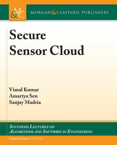
Goal State
Attack Scenario 3
Attack Scenario 4
Attack Scenario 1
Attack Scenario 2
OR
AND
Figure 4.3: An illustration of an attack graph.
Once the attack module has been developed, we can use it to implement attack graphs
for each of the WSN security parameters. By doing so, we can visualize the ways in which an
attacker might exploit the WSN security parameters. Additionally, the root node of an attack
graph is considered to be an attacker’s ultimate goal. Hence, exploitation of one of the WSN
security parameters—confidentiality, integrity, or availability, will be the root node of an attack
graph in our proposed risk assessment framework for a WSN in a sensor cloud. All other nodes
in the attack graph will be intermediate states an attacker can take during the course of their
attack. In this regard, we assume that an attack state cannot be undone once it has been exploited,
preventing any form of backtracking. erefore, we define an attack graph for a WSN in the
sensor cloud using information from the attack pattern and attack module databases as follows.
Definition 4.3 Attack graph. An attack graph is a tuple containing the attributes (s
root
, S, ,
), where s
root
is the goal of the attacker—one of the WSN security parameters. S denotes the
complete set of attacks (Table 4.2). denotes the set of pre- and post-conditions of all attacks
in S. is the join type, 2 [OR, AND].
4.2.2 QUANTITATIVE RISK ASSESSMENT BY MODELING ATTACK
GRAPHS USING BAYESIAN NETWORKS
An attack graph’s nodes maybe assigned with either true or false values implying that an attack
state is either successfully executed or not executed at all. However, to better analyze an attack
scenario and draw actionable insights from it, we can assign numerical values. An instantiation
of such numerical representation can be encapsulated in the probability of success of executing an
attack s
i
, Pr.s
i
/. e probability of success of attacks can be derived from their severity ratings
and can be estimated by adopting the scoring metric established by NIST’s CVSS.
CVSS scores are based on three criteria; base metrics, temporal metrics, and environ-
mental metrics. Base metric is used to express the level of difficulty to exploit a vulnerability.
Temporal and environmental metrics are used to express the effect of the network’s deployment
environment and surroundings in the exploitation of the vulnerability. e base metric is further
comprised of exploitability sub-score and impact sub-score. e exploitability sub-score is com-

54 4. RISK ASSESSMENT IN A SENSOR CLOUD
prised of access vector (B_AR), access complexity (B_AC), and authentication instances (B_AU).
Access vector (B_AR) depicts how a vulnerability is exploited. Access complexity (B_AC) de-
scribes the difficulty of exploiting the vulnerability. Authentication instances (B_AU) states how
many authentication is required on the attackers part in order to exploit the vulnerability. e
impact sub-score suggests the damage of the attack on parameters such as confidentiality (B_C),
integrity (B_I), and availability (B_A). Temporal metrics consists of availability of exploitabil-
ity tools and techniques (T_E). It depicts the current state of exploitation techniques available.
Remediation level (T_RL) categorizes the type of solutions available to fix the vulnerability. Re-
port confidence (T_RC) describes the evidence available on the existence of the vulnerability. e
environmental metrics quantify two aspects of impact that depend on the surrounding environ-
ment of the organization: (1) the collateral damage of the attack (E_CDP); and (2) the security
required for organizational assets such as confidentiality (B_CR), integrity (B_IR), and avail-
ability (B_AR). ese metrics are summarized in Table 4.4.
Table 4.4: CVSS metric description
CVSS Metrics Subcategories Attributes Description
Base
Exploitability sub-score
Access
Vector
Access
Complexity
Authentication
Instances
Vulnerability exploitation from
within network domain or remotely
Difi culty in exploiting vulnerability
Number of authentication measure
that needs to be bypassed
Impact sub-score
Confi dentiality
Integrity
Availability
Impact on confi dentiality
Impact on integrity
Impact on availability
Temporal
Exploitability tools
& techniques (T_{E})
Remediation level
(T_{RL})
Report Confi dence
(T_{RC})
Current state of available exploita-
tion techniques
Type of solutions available to fi x the
vulnerability
Evidences available about existence
of vulnerability
Environmental
Collateral Damage
Security required
Impact of exploited vulnerability on
organization’s economy
Amount of security required for
organizational assets like confi den-
tiality, integrity, and availability

4.2. RISK ASSESSMENT FRAMEWORK FOR WSN IN A SENSOR CLOUD 55
WSN attacks have not yet been corroborated by CVSS and as such the base metrics will
be evaluated subjectively. We also assume that, although preventive measures for the attacks are
available, they are solutions which individual researchers have reported. Hence, based on the
definition of remediation level, we have considered these solutions as workaround fixes. Envi-
ronmental metrics are context specific varying for different organizations and is constant for
any given organization. Houmb’s misuse frequency model [46] performs risk level estimations
as a conditional probability over the Misuse frequency (MF) and Misuse Impact (MI) estimates
of an attack. MF and MI of an attack helps in depicting the likelihood and impact of an at-
tack respectively taking into account the intrinsic attributes of the attack, network architecture,
and security measures used. It is useful in estimating time frames predicting the degradation
of organizational assets like confidentiality, integrity, and availability. Hence, to compute the
probability of success of attack nodes in our attack graph, we have adopted Houmb’s misuse fre-
quency model. MF of an attack is calculated using (4.1)–(4.3) and CVSS parameters specified
in Table 4.5:
MF
init
D
1
3
X
s
i
2S
.
B_fARg; B_fACg; B_fAUg
/
(4.1)
MF
uFac
D
1
3
X
s
i
2S
.
T _fEg; T _fRLg; T _fRCg
/
(4.2)
MF D
1
2
X
s
i
2S
.
MF
init
; MF
uFac
/
: (4.3)
Initial misuse frequency, MF
init
in (4.1) is calculated using exploitability sub-score under
the base metrics (Tables 4.4 and 4.5). We normalize the values of B_{AR}, B_{AC}, B_{AU} for
the attack under consideration, to keep the final score between 0!1 since the value of MF is a
probability and therefore cannot be over 1. e MF of an attack, however, may change over time
according to the availability of security solutions and techniques for executing the attacks. ese
factors are reflected using temporal metrics, computed as MF
uFac
(4.2). MF
uFac
is then added
to (MF
init
) and the final misuse frequency (MF) is computed in (4.3). Similar computations are
done to calculate MI using the impact sub-score under base metrics and environmental metrics
(Table 4.6) [54] and (4.4)–(4.7). Initial MI estimate, MI
init
, is estimated using impact sub-
score of the base metrics in (4.4). is estimate is a vector depicting the effect of an attack on
confidentiality, integrity, and availability of a network. MI
init
is then updated on the basis of the
collateral damage potential (E_CDP) in (4.5). e MI estimates are further updated as per the
security requirements information in (4.6). Finally, the resulting MI estimate, MI, is obtained
in (4.7):

56 4. RISK ASSESSMENT IN A SENSOR CLOUD
Table 4.5: CVSS vectors to calculate MF
CVSS Metrics CVSS Attributes Rating Rating Value
Base
Access vector (B_{AR})
Local (L)
Adjacent network (A)
Network (N)
0.395
0.646
1.00
Attack complexity (B_{AC})
High (H)
Medium (M)
Low (L)
0.35
0.61
0.71
Authentication instances (B_
{AU})
Multiple (M)
Single (S)
None (N)
0.45
0.56
0.704
Temporal
Exploitability tools & techniques
(T_{E})
Unproved (U)
Proof-of-Concept (POC)
Functional (F)
High (H)
0.85
0.90
0.95
1.00
Remediation level (T_{RL})
Offi cial Fix (OF)
Temporary Fix (TF)
Workaround (W)
Unavailable (U)
0.87
0.90
0.95
1.00
Report Confi dence (T_{RC})
Unconfi rmed (UC)
Uncorroborative (UR)
Confi rmed (C)
0.90
0.95
1.00
MI
init
D
Œ
B_fC g; B_fI g; B_fAg
(4.4)
MI
CDP
D E_CDP
Œ
MI
init
(4.5)
MI
Env
D
Œ
B_fCRg; B_fIRg; B_fARg
(4.6)
MI D MI
CDP
MI
Env
: (4.7)
Once we compute the MF, we can estimate an attack’s probability of success, Pr(s
i
), us-
ing (4.8):
Pr.s
i
/ D .1 /MF
init
C
.
MF
uFac
/
; (4.8)
where is a constant and is defined as the security administrator’s belief of the impact of the se-
curity measures on an attack’s MF (base metrics) and temporal metrics. It can vary from [0,0.5].

4.2. RISK ASSESSMENT FRAMEWORK FOR WSN IN A SENSOR CLOUD 57
Table 4.6: CVSS vectors to calculate MI
CVSS Metrics CVSS Attributes Rating
Rating
Value
Base
Confi dentiality Impact (B_{C})
None (N)
Partial (P)
Complete (C)
0.00
0.275
0.660
Integrity Impact (B_{I})
None (N)
Partial (P)
Complete (C)
0.00
0.275
0.660
Availability Impact (B_{A})
None (N)
Partial (P)
Complete (C)
0.00
0.275
0.660
Environmental
Condentiality Requirement (E_{CR}))
Low (L)
Medium (M)
High (H)
0.50
1.00
1.51
Integrity Requirement (E_{IR})
Low (L)
Medium (M)
High (H)
0.50
1.00
1.51
Availability Requirement (E_{AR})
Low (L)
Medium (M)
High (H)
0.50
1.00
1.51
Collateral Damage Potential (E_CDP)
None (N)
Low (L)
LowMedium (LM)
MediumHigh (MH)
High (H)
0.00
0.10
0.30
0.40
0.50
If a security administrator is uncertain about the impact of security measures of an attack (like
in cases of new or unknown attacks), then the probability of success is based on the base metrics,
by taking as 0.
After assigning attack graph’s nodes with their probability of success, we depict it as a
Bayesian network. is will help us to ascertain the non-deterministic nature of the attacks for
different network scenario with a reasonable amount of accuracy. A Bayesian attack graph in our
framework can be defined as follows.
..................Content has been hidden....................
You can't read the all page of ebook, please click here login for view all page.